nLab May spectral sequence
under construction
Context
Homological algebra
(also nonabelian homological algebra)
Context
Basic definitions
Stable homotopy theory notions
Constructions
Lemmas
Homology theories
Theorems
Stable Homotopy theory
Ingredients
Contents
Contents
Idea
A May spectral sequence (May 64, May 74, Ravenel 86, 3.2) is a certain type of spectral sequence that computes the second page of the classical Adams spectral sequence. More generally, it computes Ext-groups (or Cotor-groups, via this lemma) of comodules over commutative Hopf algebras (the dual Steenrod algebra in the classical case) starting from the corresponding -groups over just an associated graded Hopf algebra.
The May spectral sequence is the spectral sequence of a filtered complex induced by suitably filtering the canonical (but intractable) bar complex model for Ext/Cotor (see Ravenel 86, chapter 3, section 2, Kochman 96, section 5.3).
Preliminaries
Cobar complex
Proposition
Given a graded commutative Hopf algebroid, then becomes a left comodule over with coaction given by the right unit
and it becomes a right comodule with coaction given by the left unit
Proof
Dually this is the action of morphisms on objects given by evaluation at the source or target, respectively.
Definition
Let be a commutative Hopf algebra, hence a commutative Hopf algebroid for which the left and right units coincide .
Then the unit coideal of is the cokernel
Lemma
Let be a commutative Hopf algebra, hence a commutative Hopf algebroid for which the left and right units coincide .
Then the unit coideal (def. ) carries the structure of an -bimodule such that the projection morphism
is an -bimodule homomorphism. Moreover, the coproduct descends to a coproduct such that the projection intertwines the two coproducts.
Proof
For the first statement, consider the commuting diagram
where the left commuting square exhibits the fact that is a homomorphism of left -modules.
Since the tensor product of abelian groups is a right exact functor it preserves cokernels, hence is the cokernel of and hence the right vertical morphisms exists by the universal property of cokernels. This is the compatible left module structure on . Similarly the right -module structure is obtained.
For the second statement, consider the commuting diagram
Here the left square commutes by one of the co-unitality conditions on , equivalently this is the co-action property of regarded canonically as a -comodule.
Since also the bottom morphism factors through zero, the universal property of the cokernel implies the existence of the right vertical morphism as shown.
Definition
(cobar complex)
Let be a commutative Hopf algebra, hence a commutative Hopf algebroid for which the left and right units coincide . Let be a left -comodule.
The cobar complex is the cochain complex of abelian groups with terms
(for the unit coideal of def. , with its -bimodule structure via lemma )
and with differentials given by the alternating sum of the coproducts via lemma .
Proposition
Let be a commutative Hopf algebra, hence a commutative Hopf algebroid for which the left and right units coincide . Let be a left -comodule.
Then the cochain cohomology of the cobar complex (def. ) is the Ext-groups of comodules from (regarded as a left comodule via def. ) into
(Ravenel 86, cor. A1.2.12, Kochman 96, prop. 5.2.1)
Self-Ext of free graded commutative coalgebras
Throughout, let be a commutative ring and let be a graded commutative Hopf algebra over . We write for this data.
Lemma
Let be a graded commutative Hopf algebra such that
-
the underlying algebra is free graded commutative;
-
is a flat morphism;
-
is generated by primitive elements
then the Ext of -comodules from and itself is the (graded) polynomial algbra on these generators:
(Ravenel 86, lemma 3.1.9, Kochman 96, prop. 3.7.5)
Proof
Consider the co-free left -comodule (prop.)
and regard it as a chain complex of left comodules by defining a differential via
and extending as a graded derivation.
We claim that is a homomorphism of left comodules: Due to the assumption that all the are primitive we have on generators that
and
Since is a graded derivation on a free graded commutative algbra, and is an algebra homomorphism, this implies the statement for all other elements.
Now observe that the canonical chain map
(which projects out the generators and and is the identity on ), is a quasi-isomorphism, by construction. Therefore it constitutes a co-free resolution of in left -comodules.
Since the counit is assumed to be flat, and since is trivially a projective module over itself, this prop. now implies that the above is an acyclic resolution with respect to the functor . Therefore it computes the Ext-functor. Using that forming co-free comodules is right adjoint to forgetting -comodule structure over (prop.), this yields:
Lemma
If is equipped with a filtering right/left -comodules and are compatibly filtered, then there is a spectral sequence
converging to the Ext over between and , whose first page is the Ext over the associated graded Hopf algebra between the associated graded modules and .
(Ravenel 86, lemma 3.1.9, Kochman 96, prop. 3.7.5)
Proof
The filtering induces a filtering on the standard cobar complex (def. ) which computes . The spectral sequence in question is the corresponding spectral sequence of a filtered complex. Its first page is the homology of the associated graded complex (by this prop.).
Construction of the May spectral sequence
Let now , be the mod 2 dual Steenrod algebra. By Milnor’s theorem, as an -algebra this is
and the coproduct is given by
where we set .
Definition
Set
Also one abbreviates
By binary expansion of powers, there is a unique way to express every monomial in as a product of the elements from def. , such that each such element appears at most once in the product. E.g.
Proposition
In terms of the generators , the coproduct on takes the following simple form
Proof
Using that the coproduct of a bialgebra is a homomorphism for the algebra structure and using freshman's dream arithmetic over , one computes:
Define a grading on by setting (this is due to (Ravenel 86, p.69))
and extending this additively to these unique representative.
For instance
Consider the corresponding filtering
with filtering stage containing all elements of total degree .
Observe that
This means that after projection to the associated graded Hopf algebra
all the generators become primitive elements:
Hence lemma applies and says that thet from to itself over the associated graded Hopf algebra is the polynomial algebra in these generators:
Moreover, lemma says that this is the first page of a spectral sequence that converges to the over the original Hopf algebra:
This is the May spectral sequence for the computation of . Notice that since everything is -linear, its extension problem is trivial.
Moreover, again by lemma , the differentials on any -page are the restriction of the differentials of the bar complex to the -almost cycles (prop.). The differential of the bar complex is the alternating sum of the coproduct on , hence by prop. this is:
The second page of the classical Adams spectral sequence
Now we use the above formula to explicitly compute the cohomology of the second page of the classical Adams spectral sequence.
In doing so it is now crucial that the differential in the standard cobar complex (def. ) for lands in where the generator disappears.
Recall the further abbreviation
Hence we find using the formula from prop. , that
and hence all the elements are cocycles.
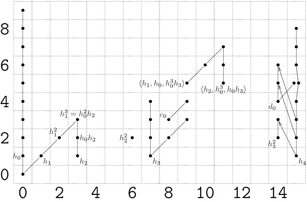
Lemma
In the range , the second page of the May spectral sequence for has as generators all the
as well as the element
subject to the relations
-
.
The differentials in this range are
-
.
e.g. (Ravenel 86, lemma 3.2.8 and lemma 3.2.10, Kochman 96, lemma 5.3.2 and lemma 5.3.3)
Hence this solves the May spectral sequence, hence gives the second page of the classical Adams spectral sequence. Inspection just of the degrees then shows that in this range there is no non-trivial differential in the Adams spectral sequece in this range. This way one arrives at:
Theorem
In low the group is spanned by the items in the following table
(graphics taken from (Schwede 12))
(Ravenel 86, theorem 3.2.11, Kochman 96, prop. 5.3.6)
Hence the first dozen stable homotopy groups of spheres 2-locally are
| 0 | 1 | 2 | 3 | 4 | 5 | 6 | 7 | 8 | 9 | 10 | 11 | 12 | 13 | |
|---|---|---|---|---|---|---|---|---|---|---|---|---|---|---|
Remark: The full answer turns out to be this:
| 0 | 1 | 2 | 3 | 4 | 5 | 6 | 7 | 8 | 9 | 10 | 11 | 12 | 13 | 14 | 15 | ||
|---|---|---|---|---|---|---|---|---|---|---|---|---|---|---|---|---|---|
Related concepts
References
The origin is in
-
Peter May, The cohomology of restricted Lie algebras and of Hopf algebras; application to the Steenrod algebra, Thesis, Princeton 1964
-
Peter May, The cohomology of restricted Lie algebras and of Hopf algebras, Journal of Algebra 3, 123-146 (1966) (pdf)
-
Peter May, Some remarks on the structure of Hopf algebras, Proceedings of the AMS, vol 23, No. 3 (1969) (pdf)
Further computational improvements and a computation of the first 70 differentials (for the case of the mod 2 Steenrod algebra) was given in
- Martin Tangora, On the cohomology of the Steenrod algebra, Math. Z. 116, 18-64 (1970)
More on the -term is in
- Peter May, The Steenrod algebra and its associated graded algebra, University of Chicago preprint, 1974.
Review includes
-
Doug Ravenel, chapter 3, section 2 of Complex cobordism and stable homotopy groups of spheres, 1986
-
Stanley Kochman, section 5.3 of Bordism, Stable Homotopy and Adams Spectral Sequences, AMS 1996
-
Wikipedia, May spectral sequence
Last revised on October 15, 2020 at 01:21:47. See the history of this page for a list of all contributions to it.