John Baez Petri net field theory

Abstract

Stochastic processes, such as diffusion limited reactions arise in diverse fields of science and engineering. Powerful analytical methods and numerical techniques have been developed to simulate various phenomena associated with such processes, but very little is known about the precise connections and interrelations between the techniques themselves. The modern theory of categories provides a catalyst for such a study. Here we expose the connection between two a priori seemingly different tools: Petri nets and field theory. The combination of these approaches unifies the modelling of diffusion limited reactions. These methods fit together naturally in the language of monoidal categories.

Introduction and background

There has been work geared towards modelling diffusion limited reactions as well as predator prey scenarios using field theory techniques and independently, Petri networks. However, the precise connection between these diverse approaches has remained unknown. One can arrive at a unification of these ideas by exploring the high-level mathematical structure of these models. This connection is made vivid by considering Petri nets as instances of monoidal categories and by mapping the induced evolution to a suitable Fock space. This is precisely what this page describes.

This project is part of our larger effort to understand the mathematical structure of networks at various levels of abstraction and to pinpoint interrelations. Related ideas to what we explore here can be found in

• John Baez, Electrical Circuits. (nLab, 2010)

• John C. Baez, James Dolan, From Finite Sets to Feynman Diagrams, In Mathematics Unlimited - 2001 and Beyond, vol. 1, eds. Bjorn Engquist and Wilfried Schmid, Springer, Berlin, 2001, pp. 29-50. http://arxiv.org/abs/math/0004133.

Outline

We assume that readers are familiar with stochastic processes at only a basic level. For background information on these ideas, we recommend becoming familiar with the blog entry

• n-Category Cafe on attractors and predator prey models

We wish to study stochastic processes using Petri nets. A blog entry developed for this purpose can be found here

• Blog about Petri nets, Azimuth blog.

with basic background found on the Azimuth project

• Petri nets, Azimuth project.

Because there are already blog articles about predator prey interactions as a stochastic process as well as Petri nets, we will focus on the missing pieces here, namely the field theory methods needed to model stochastic Petri nets.

Fock space basis

We consider a subspace of the Fock space basis formed by the symmetric algebra of polynomials formed over monomials.

$$S C^2 = \{ \sum_{n,m=1}^\infinity \alpha_{n,m}x^n y^m\}$$

We let

$$\partial_x := \frac{\partial}{\partial x}$$

and

$$\partial_y := \frac{\partial}{\partial y}$$

then $\partial_x^+$ becomes multiplication by $x$ which sometimes appears in the mathematics literature as $m_x$. Likewise

$$\partial_y^+ := y$$

which is sometimes denoted as $m_y$.

We then adopt the standard short hand notation and introduce letters $a^-$, $a^+$ etc. as notation for $\partial_x$, $\partial_x^+$. We then let these operators act on our basis as

$$a_x x^n = n x^{n-1}$$

that is

$$a_x |n\rangle = \sqrt{n}|{n-1}\rangle$$

and

$$a_x^+ x^n = x^{n+1}$$

that is

$$a_x^+ |n\rangle = \sqrt{n+1}|n+1\rangle$$

where

$$\langle{n}|{m}\rangle = \delta_{nm}$$

and we relate $x^n$ to $|n\rangle$ as

$$\langle x^0|x^0\rangle= 1$$

$$\langle x^n|x^n\rangle= n!$$

$$||x^n|| = \sqrt{n!}$$

and hence

$$x^n = \sqrt{n!}|n\rangle$$

The result above is known and follows from $\langle x^n|x^n\rangle=\langle x^n| a^+_x x^{n-1}\rangle = \langle a_x x^n| x^{n-1}\rangle = n \langle x^{n-1}|x^{n-1}\rangle$.

A categorical comment

We could have proceeded by considering the free symmetric monoidal category on 2 objects $x$ and $y$. We then decategorify by considering the set of isomorphism classes of objects, the set

$$\{x^n y^m\}_{n,m\in N}$$

resulting in a free commutative monoid on 2 elements $x$ and $y$. We then linearise by taking linear combinations. $S(C^2)$ iso Fock space on $C^2$.

For a related reference see: http://onlinelibrary.wiley.com/doi/10.1002/prop.19800281004/pdf

The evolution equation

The Master Equation takes the form

$$\partial_t |X(t)\rangle = - H|X(t)\rangle$$

where H is expressed in terms of the raising and lowering operators. This equation is formally solved per introduction of an integrating factor $e^{tH}$ as

$$e^{tH}(\partial_t + H)|X(t)\rangle = 0$$

and hence

$$|X(t)\rangle = e^{-tH}|X(0)\rangle$$

Wolf and rabbit field theory

The free wolf field

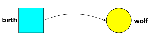
Exponential growth. In this toy model, wolves do not die, but can be born with some probability.

We will consider the chemical mass-action kinetic equation as follows

$$\frac{dX}{dt}= \alpha - \beta X$$

This is depicted as

$$\phi \to x$$

We map this to a Hamiltonian:

$$H = \alpha a^+$$

and consider starting the system in the zero-wolves state

$$\psi_n(0) = x^0 = 1$$

The evolution then becomes

$$\psi_n(t)= e^{\alpha H t} \psi_n(0)$$

From the exponential formula, this gives a history state over all possible worlds. A wolf mosaic if you will.

This equation gives probability of there being a different number of $k$ wolves at some time $t$ indexed by the power of $x$ as

$$\sum_{n=0}^\infinity \frac{1}{n!}\alpha^n\t^n x^n$$

An infinite state space of possibilities is occupied for $t$ > $0$. The sum of the coefficients grows exponentially with time. The normalisation is given as

$$\sqrt{(\psi_n,\psi_n)} = e^{\alpha t}$$

The probability of their being n wolves at time t is then given as

$$P_n(t)= \frac{\alpha^n t^n}{n!} e^{-\alpha t}$$

Petri net for exponentially growing population.

Exponential death. In this toy model, wolves are not born, and an initial population dies with with some probability.

Lotka-Volterra models

• http://www.stolaf.edu/people/mckelvey/envision.dir/lotka-volt.html
• http://en.wikipedia.org/wiki/Lotka%E2%80%93Volterra_equation
• http://www.scholarpedia.org/article/Predator-prey_model
• http://iopscience.iop.org/0295-5075/88/6/68002/pdf/epl_88_6_68002.pdf
• http://math.bu.edu/people/isaacson/rdme_asympt.pdf

In particular:

• http://www.phys.vt.edu/~tauber/08_68_comenc.pdf

References

We are still conducting a literature search into this area. These papers discuss the use of second quantization for systems of identical classical objects:

• M. Doi, Second quantization representation for classical many-particle systems, J. Phys. A 9 (1976), 1465-1477.

• P. Grassberger, M. Scheunert,Fock-Space Methods for Identical Classical Objects_, Fortschritte der Physik, Volume 28, Issue 10, pages 547–578, 1980. PDF.

Abstract: “Fock-Space (annihilation/creation operator) methods are introduced to describe systems of identical classical objects. Specific examples to which this formalism is applied are branching processes (including age dependent ones), chemical reactions, deterministic (Hamiltonian) systems, and generalized kinetic equations. Finally, a generalization to stochastic quantum systems is proposed which is applied to a gas of spinning molecules.”

These papers discuss applications to diffusion-limited reactions:

• M. Doi, Stochastic theory of diffusion-controlled reactions, J. Phys. A 9 (1976) 1479-1495.

• Daniel C. Mattis and M. Lawrence Glasser, The uses of quantum field theory in diffusion-limited reactions, Reviews of Modern Physics, 70 (1998)979-1001. http://adsabs.harvard.edu/abs/1998RvMP…70..979M

• Martin J Howard and Uwe C. Täuber, Real versus imaginary noise in diffusion-limited reactions, J. Phys. A 30 (1997) 7721 10.1088/0305-4470/30/22/011.

• There was a course given on Nonequilibrium Statistical Mechanics: Fundamental Problems and Applications. See the 4 lectures by Vollmayr-Lee, entitled Field theory approach to diffusion-limited reactions. course homepage

• Mobilia, Mauro; Georgiev, Ivan T.; Täuber, Uwe C., Fluctuations and correlations in lattice models for predator-prey interaction, Physical Review E 73 (????) 040903. DOI: 10.1103/PhysRevE.73.040903

• Mauro Mobilia, Ivan T. Georgiev, and Uwe C. Tauber, Phase transitions and spatio-temporal fluctuations in stochastic lattice Lotka-Volterra models, arXiv:q-bio/0512039.

This paper has a fairly up-to-date review of previous work:

• Uwe Claus Täuber, Field-theoretic Methods, arXiv:0707.0794.

This section on history is interesting:

More than thirty years ago, Janssen and De Dominicis independently derived a mapping of the stochastic kinetics defined through nonlinear Langevin equations onto a field theory action (Janssen 1976 [35], De Dominicis 1976 [36]; reviewed in Janssen 1979 [11]). Almost simultaneously, Doi constructed a Fock space representation and therefrom a stochastic field theory for classical interacting particle systems from the master equation describing the corresponding stochastic processes (Doi 1976 [37, 38]). His approach was further developed by several authors into a powerful method for the study of internal noise and correlation effects in reaction-diffusion systems (Grassberger and Scheunert 1980 [39], Peliti 1985 [40], Peliti 1986 [41], Lee 1995 [42], Lee and Cardy 1995 [43]; for recent reviews, see Refs. [12, 13]). We shall see below that the field-theoretic representations of both classical master and Langevin equations require two independent fields for each stochastic variable. Otherwise, the computation of correlation functions and the construction of perturbative expansions fundamentally works precisely as sketched above. But the underlying causal temporal structure induces important specific features such as the absence of ‘vacuum diagrams’ (closed response loops): the denominator in Eq. (2) is simply Z = 1. (For unified and more detailed descriptions of both versions of dynamic stochastic field theories, see Refs. [14, 15].)

• John Baez and Jacob Biamonte, Graphical networks, nLab.

• John Baez, Mathematical Economics, Azimuth blog.