nLab Hegelian taco

Idea

The Hegelian taco is food for thought from William Lawvere's kitchen. More concretely, it is an eight-element graphic monoid that intends to capture diagrammatically the essence of a certain configuration of stacking subcategories of a given category that occurs in Lawvere’s mathematical rendering of Hegel's dialectical logic.

Construction

The situation we start with is the following sequence of functors and adjunctions

$$\mathcal{A}\overset{\hookleftarrow}{\underset{\hookleftarrow}{\to}} \mathcal{B}\overset{\hookleftarrow}{\underset{\hookleftarrow}{\to}}\mathcal{C}\overset{\hookleftarrow}{\underset{\hookleftarrow}{\to}} 1$$

Here every column of arrows, numbered descendingly $2, 1, 0$ from left to right describes an essential localization $j_n\dashv f_n\dashv i_n$ with $j_n,i_n$ fully faithful. These yield a pair of idempotent adjoint modalities whose functor parts are $j_n f_n\dashv i_n f_n$. Importantly, all the junctures vanish in the sense $f_n i_n=1$, since this composition corresponds to the inclusion of a subcategory followed by a projection back to the subcategory.

If we compose the functors appropriately we obtain four such adjunctions on $\mathcal{A}$ which correspond to reflective and coreflective embeddings of descending complexity of the chain of subcategories $\mathcal{A}\supset\mathcal{B}\supset\mathcal{C}\supset 1$:

$$\begin{aligned} id_\mathcal{A}&\dashv id_\mathcal{A} \\ L &\dashv R \\ l &\dashv r \\ 0 &\dashv 1 \end{aligned}$$

The respective endofunctors on $\mathcal{A}$ are defined as

$$\begin{aligned} 1&:=i_2 i_1 i_0 f_0 f_1 f_2 \\ 0&:=j_2 j_1 j_0 f_0 f_1 f_2 \\ r&:=i_2 i_1 f_1 f_2\\ l&:=j_2 j_1 f_1 f_2\\ R&:=i_2 f_2\\ L&:=j_2 f_2 \end{aligned}$$

They are supposed to provide the elements of the taco monoid $M$. So far we have seven of them including $id_\mathcal{A}$. The eighth will show up when we set up the multiplication table, so let’s do that:

1. The first case we consider is when we multiply two elements that appear on the same side of $\dashv$ like e.g. $L$ and $l$ that are both left adjoints: here $l$ is of lower complexity than $L$ as it corresponds to a smaller subcategory, namely $\mathcal{C}$. When we multiply, ${l}L$ or $L{l}$, at the junctures will arise in both cases $f_2 j_2$ which is just the ‘splitting’ of $L$ and therefore cancels and we retain the ‘lower’ functor $l={l}L=L{l}$. This happens in all cases where we multiply elements of the same ‘laterality’: the lower element absorbs the higher. This can be viewed as capturing the facet of ‘preservation’ present in Hegelian Aufhebung: the higher concept $L$ is just $l$ when restricted to the smaller subcategory.

2. Next we come to the cases where we multiply elements of opposite laterality of the same complexity e.g. like $L$ and $R$. Here the factors arising at the junctures cancel again and in these cases we retain always the left factor e.g. $L{R}=L$ and $R{L}=R$. One can view this as capturing the destructive nature of a Hegelian ‘dialogue’: ‘objecting’ $L$ to ‘proposal’ $R$ cancels $R$ and vice versa.

3. Now we come to the cases that express the constructive-progressive nature of Hegelian dialectic: namely, when we multiply elements of opposite laterality of different complexity e.g. like $R$ and $l$. Let us concentrate on the case that the difference in complexity is just a single step. First we note, that the dialogue situation is conceived of as being asymmetrical: the right adjoint acts as proponent whereas the left adjoint opponent contradicts. So in this particular formalization, the proponent tries to assimilate the opponent’s view but not vice versa: in a ‘situation’ $l{r}=l$ where the ‘proponent’ $r$ is faced with ‘opposition’ $l$, she might just insist $r{l}r=r{l}=r$ but she might as well try to take $l$ into account i.e. change her view $r$ to $R$, with the ‘higher order refinement’ $R$ now ‘accepting’ $l$ in the sense that $R{l}=l$. This relation that $L_i$ not only factors through $L_{i+1}$ but through $R_{i+1}$, is called resolution of (the contradiction of) level $n$ by level $n+1$ (For further details see at Aufhebung). It gives us the equations ${r}0=0$ , $R{l}=l$, and (trivially) $id {L}=L$ for the three steps of sublations.

As we’ve said, the situation is handled somewhat asymmetrical in that we systematically care only that we can incorporate the negative view into the positive ‘right adjoint’ view but not the reverse. For the reverse cases ${l}1$ and ${L}r$ we stipulate: 1) ${l}1=1$ (this would hold, as often occurs in the applications, that there is an additional left adjoint $\pi\dashv j_2j_1\dashv f_1f_2$ since in that case $l$ as a composition of right adjoints would preserve the limit $1$) and 2.) $q:={L}r$ which give us our eighth element!

So much for the ‘philosophical’ motivation behind the multiplication table that is going to follow in the next section!

Some might feel more comfortable with the information that, technically, the taco monoid intends to abstract the relations occuring between three essential localizations such that, starting from $0\dashv 1$, a higher localization resolves the preceding lower level in the sense that $R_{n+1} L_n= L_n$.

Definition

The Hegelian taco is the monoid on the set $\{id,0,1,l,r,L,R,q\}$ with the following multiplication table:

$$\array{ && 0 & 1 & l & q & r & L & R & id \\ &&&&&&&&&\\ 0 && 0 & 0 & 0 & 0 & 0 & 0 & 0 & 0 \\ 1 && 1 & 1 & 1 & 1 & 1 & 1 & 1 & 1 \\ l && 0 & 1 & l & l & l & l & l & l \\ q && 0 & 1 & q & q & q & q & q & q \\ r && 0 & 1 & r & r & r & r & r & r \\ L && 0 & 1 & l & q & q & L & L & L \\ R && 0 & 1 & l & r & r & R & R & R \\ id&& 0 & 1 & l & q & r & L & R & id }$$

Properties

$M$ is a graphic monoid i.e. for all $x,y\in M$ we have $x y x=x y$, in particular all elements are idempotent.

The poset of left ideals in $M$ is:

$$\emptyset\subset \{ 0,1 \} \subset \{ 0,1,l,q,r \} \subset \{ 0,1,l,q,r,L,R \} \subset \{ 0,1,l,q,r,L,R,id \}$$

They parametrize the essential localizations of the associated presheaf topos $Set^{M^{op}}$. The dimension theory that comes with this is detailed in Kelly-Lawvere (1989) and Lawvere (1989). In the present case, the result is that $Set^{M^{op}}$ is three-dimensional.

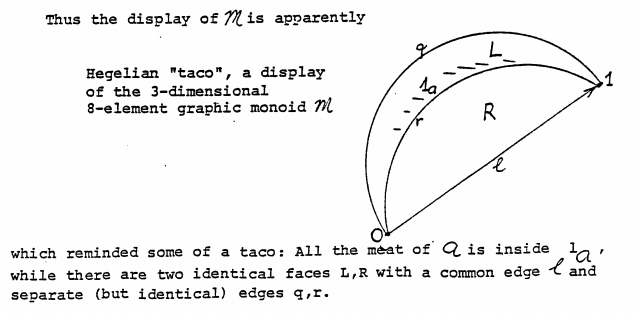
This motivates also the culinary allusion in the name, where the essential localization corresponding to $\mathcal{B}$ is seen as providing the two-dimensional ‘sides’ via its reflective and coreflective inclusions around the three-dimensional ‘filling’ $\mathcal{A}$. Of course, the one-dimensional pieces $l,q,r$ corresponding to $\mathcal{C}$ find their place on the sandwich as well. The following picture of the taco appears in Lawvere (1989), where further details may be found.

Let us point out that $M$ can be viewed as ‘cubical generalization’ of the three-element graphic monoid $\Delta_1$ that underlies the (one-dimensional) presheaf topos of reflexive graphs (for a detailed description of $\Delta_1$ and its topos see at graphic category). $\Delta_1$ encapsulates the diagram

$$\mathcal{A}\overset{\hookleftarrow}{\underset{\hookleftarrow}{\to}} \mathcal{B}$$

that expresses abstractly a cylinder configuration corresponding to ‘opposition’ or ‘conflict’ from the dialogical point of view.¹

Remarks

• If one takes into account also the natural transformations arising from the adjunctions one can turn $M$ into a finite monoidal category.

• The main reference for the taco is Lawvere (1989, pp.70-73). It is mentioned in Lawvere (1991,2003) as well.

Related entries

• graphic category

• graphic topos?

• shelf

• Aufhebung

• graph

• Science of Logic

• adjoint cylinder

• 2-category of adjunctions

• Adj

References

• G. M. Kelly, F. W. Lawvere, On the complete lattice of essential localizations , Bull. Soc. Math. de Belgique XLI (1989) 289-319 [pdf]

• F. W. Lawvere, Display of graphics and their applications, as exemplified by 2-categories and the Hegelian “taco” Proceedings of the first international conference on algebraic methodology and software technology University of Iowa, May 22-24 1989, Iowa City, pp. 51-74. (pdf)

• F. W. Lawvere, More on graphic toposes, Cah. Top. Géom. Diff. Cat. XXXII no. 1 (1991) pp.5-10. (pdf)

  ‎

• F. W. Lawvere, Unity and identity of opposites in calculus and physics , App. Cat. Struc 4 (1996) pp.167-174. (pdf)

• F. W. Lawvere, Linearization of graphic toposes via Coxeter groups, JPAA 168 (2002) pp. 425-436. (pdf)

---

1. Lawvere expands a bit on the diagrammatic perspective on $\Delta_1$ in Lawvere (1996). ↩