Schreiber Notes

The following are notes in preparation of a podcast discussion. The idea is to explain purely verbally and leisurely, to a broad and lay audience, basic concepts not only of category theory and topos theory but of their interplay with Hegelian ontology. This is a tall order. We need to assume that the audience, even if lay, has some inclination towards such esoteric topics. But we motivate the development from a fundamental open questions in contemporary theoretical physics and indeed aim the development at the cohesive topos theory that serves, as we try indicate, as a rigorous metaphysics for complete non-perturbative quantum field theory.

Motivation: From Complete QFT via Toposes to Ontology, and back

Why care about higher category and topos theory in physics?

Here we have a physics mindset, the attitude of “natural philosophy” in the old sense: We primarily care about understanding the world. This entails embracing the foundational mathematics that naturally comes with this endeauvor; and disregard mathematics that is just an end in itself.

Cohesive higher Topos Theory turns out to be the right math that provides the backdrop for the geometry of physics. As in: What really is a space of gauge fields, globally and non-perturbatively?

As such, topos theory literally provides a mathematical metaphysics.

It is entertaining, at least, that this hard metaphysics happens to have striking resemblance to the Science of Logic poetically foreseen long ago by GWFH, a connection that was first realized by F. W. Lawvere.

But before we get to that, let’s step back and see why physics needs topos theory:

The Millennium Problem of Physics

Glory and misery of contemporary QFT: Perturbation theory. Works wonders as far as it goes; but goes only infinitesimally far.

Mathematically, perturbation theory is the geometry of infinitesimal spaces. Highly restrictive and of dubious predictivity (non-convergence…), but amenable to traditional algebra and analysis (formal power series).

The Millennium Problem of Physics: Complete QFT. Non-perturbative and globally defined. As in the slogan: “M-theory is (going to be) the completion of 11D SuGra”.

Traditionally lacking: Any concept of what such complete theories would actually be.

Requires differential geometry of global field spaces, beyond the infinitesimal. But field spaces are generically not even infinite-dimensional manifolds, thus outside the scope of traditional diff geo textbooks.

Underappreciated show stopper right there: Even basic notions that would be needed are traditionally missing. (Like: What is non-perturbative global BV-BRST??)

Toposes for the Geometry of Physics

Claim: Cohesive Higher Topos Theory is the missing globally complete Geometry of Physics.

Just like Riemannian geometry is the languge of gravity, or differential forms is the language of electromagnetic fields, or group/representation theory is the language of symmetry. You can do without, but you won’t get very far.

Topos means “place”. Where physics may take place.

First of all, a topos is a category of generalized spaces:

• a collection of “objects” $X$ — the spaces

• a collection of “morphisms” $X \xrightarrow{f} Y$ — the maps

• a composition operation $(-) \circ (-)$ on composable morphisms, which is associative and unital.

Specifically, a (Grothendieck) topos is a category of such generalized spaces which are characterized by how they are probed by a given collection of probe spaces.

A rather physics-style operational notion: Instead of traditionally defining space as a set of points with extra structure and properties, for a topos a space $X$ is defined by the system of sets of maps $U \to X$ of probe spaces $U$ into it.

Previous champion of toposes for physics: William Lawvere (see there): Started out working on continuum mechanics. Went from asking “What is a vector field, really?” to laying foundations for topos theory, in order to speak about “Toposes of Laws of Motion” (technical term: synthetic differential geometry). A language for differential equations on generalized (field) spaces.

Great start, but for modern physics we need to go further.

Higher Toposes for Generalized Symmetry

Beyond classical continuum mechanics, there is, of course:

• gauge fields,

• topological charges,

• orbifolding (symmetry protection),

and last not least:

• quantum states.

Adjoining these to the picture brings in higher topos theory, which is geometric homotopy theory.

geometry of physics	topos theory
gauge principle	higher homotopy

A higher topos is where generalized symmetries take place.

In a higher topos, for every higher (“categorical”) gauge group $G$ there is a moduli space (moduli stack) $\mathbf{B}G$ such that for every space(time) $X$:

• a map $X \xrightarrow{ \vdash P } \mathbf{B}G$ is equivalently a $G$-principal bundle on $X$ (a charge sector of $G$-gauge fields)

• a homotopy between these is equivalently a gauge transformation.

• a higher homotopy is equivalently a higher gauge transformation.

• and so on.

In a precise sense, $\mathbf{B}G$ is the groupoid with a single object carrying $G$-worth of symmetries:

Generally, the spaces in a higher topos are like geometric sets with gauge symmetries (like orbifolds):

• in addition to elements $x$

• they contain gauge transformations

• and higher gauge-of-gauge transformations

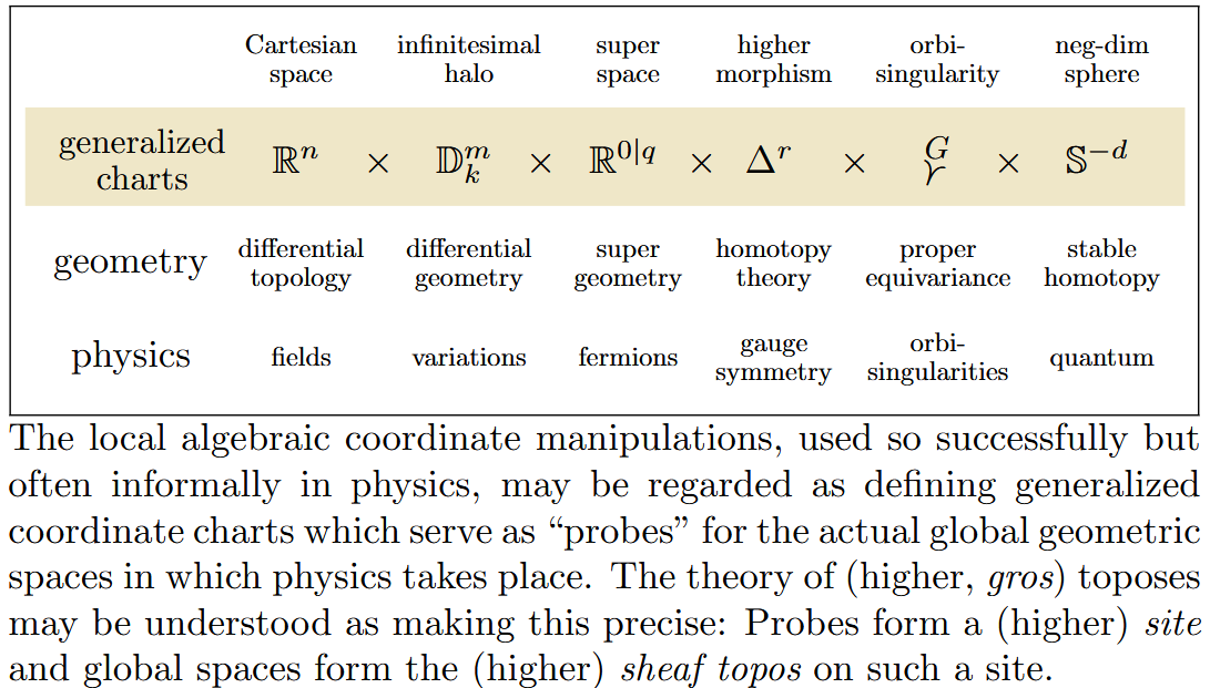
Gros Toposes for Generalized Geometry

Recall that every topos is a category of geometric spaces of some sort. (Defined by the nature of the given probe spaces.)

But many toposes (including those traditionally highlighted in introductions to the topic, unfortunately) are just categories of covering spaces of a fixed space $X$. These are clearly too small a scenery for general physics, in fact they are technically called: petit toposes.

Other toposes are categories of all generalized spaces exhibiting a given notion of geometry (differential, infinitesimal, analytic, super, … etc.). These are called gros toposes. These are potentially geometries of physics.

Here the probe spaces are generalized charts.

Cohesive $\infty$-Toposes for Higher Gauge Fields

Thus to ask: What types of gros higher toposes are actual geometries of physics?

These must contain:

• besides concrete spaces (physical spacetime)

also

• superspaces (of fermionic fields)

as well as

• moduli spaces of gauge fields.

These geometric qualities of spaces turn out to be witnessed by special higher toposes called cohesive.

These are higher toposes realizing a progression of “adjoint idempotent monads”.

Prime example:

• shape

  for every space $X$ there is its path infinity-groupoid $\esh X$:

  $n$-morphisms are $n$-dimensional paths in $X$

  original space includes as the constant path $X \xrightarrow{\eta^{\esh}} \esh X$

• points

  for every moduli space $\mathbf{A}$ there is a its underlying groupoid of points $\flat \mathbf{A}$

  devoid of their cohesion / path-connection

  includes back into the original space $\flat \mathbf{A} \xrightarrow{\epsilon^{\flat}} \mathbf{A}$

These two aspects of spaces (shape/points) are dual opposites to each other:

There is an adjunction

$$shape \dashv points$$

namely a natural bijection of maps, like this:

$$\begin{array}{rccc} & \esh X &\xrightarrow{ \nabla }& \mathbf{B}G \\ \Leftrightarrow & X &\xrightarrow{}& \flat \mathbf{B}G \end{array}$$

But maps $\esh X \xrightarrow{ \nabla } \mathbf{B}G$ encode parallel transport in the underlying $G$-bundle $X \xrightarrow{\eta^{\esh}} \esh X \xrightarrow{\nabla} \mathbf{B}G$. This is the same as a flat connection on $P$, a gauge field.

The adjunction above says that a flat connection on a $G$-principal bundle is equivalent to a reduction of its structure group to the underlying discrete group. This is a theorem of gauge theory. But here it is part of the BIOS of cohesive higher toposes.

Hard Metaphysics

Every topos is also a language of formal logic (namely of the laws that govern its geometry of physics). In this logic, the cohesive modalities are a progression of resolution of oppositions.

From this logical perspective these neatly matches idealistic ontology (“objective logic”).

So, in asking for fundamental physics we end up asking about natural foundations of mathematics.

Seems only natural: That the most fundamental physics involves the most fundamental math.

Hegel said his aim to bring philosophy closer to a form of science. The philosophy in question here is ontology, hence metaphysics (as in the old natural philosophy).

Hence to make metaphysics a hard science.

Hegel’s idealism refers to the aim that basic qualities of being (like shape and points, above) be systematically derivable from first principles (“objective logic”: a logic of how objective reality comes into being). To see how they are hard-coded in the BIOS of reality.

Hence to make metaphysics a mathematical since.

Lawvere observed/claimed that modal topos theory (my paraphrase) does provide this “objective logic” that Hegel was intuiting.

The Exceptional within the General Abstract

Two facets: The general abstract and the exceptional particular.

Example: Category of groups is general abstract. In there we find the exceptional groups.

Similarly: Solid cohesive toposes accommodate all supergeometry. In there 11D supergravity with its 5-brane is an exceptional structure.

And in higher cohesive topos, 11D supergravity does find a global completion (at least in topological sector).

Invitation to Categories

Preview

The first thing we highlight is that category theory is the theory of duality.

Of course, its basic notions are that of “categories”, “functors” and “natural transformation” (to be introduced in a moment), but by themselves, these are just an organizing principle for mathematical concepts. That organizing principle, of course, is what the term “category” is referring to.

Which is already useful, no question. For example, Geroch 1985: Mathematical Physics is a textbook that is largely concerned with showing how key mathematical concepts used in mathematical physics are organized into categories (Vector spaces, Lie algebras, Lie groups, Topological spaces, …).

But the actual theory supported by categories, as a body of powerful theorems, begins only in the next step, with the notion of adjunction, which is really a general notion of duality.

All the universal constructions that drive category theory as an actual theory are instances of such adjunctions: (Co)Limits, (Co)Ends, Kan extensions, …

This important fact is sometimes overlooked by beginners (and not so beginners), who see just the basic concept formation of categories, functors, and natural transformations and wonder what all the fuss is about and that category theory seems to have “no theorems”. Indeed, that’s because the actual theory starts only in the next step, with adjunctions and the universal constructions that these encode.

Categories

So what is a category? First of all, it is a set (possibly large, a class) of things, like in set theory. For instance, vector spaces make a category, or Lie algebras make a category. There are more exotic kinds of categories (non-concrete categories), but to begin with it is good to think of a category literally as a “category of mathematical structures”.

So what is the difference then to a set (or class)? It’s that categories actually know about the structure of these mathematical structures. Beyond just collecting all these structures indiscriminently in a large bag, in a category the nature of these structures is “transparently alive”.

So how does this work? The key idea here is structuralism: The idea that to know the nature of a mathematical object is to know how it relates to all other objects of its kind (namely: in its category!); and by that we mean: To know the homomorphisms between these objects, namely the ways of consistently “mapping them” or “transforming them” into each other.

For instance, consider a topological space $X$, an object of the category $Top$ of topological spaces. (Think of a manifold, if you like, for instance think of the 2-sphere.) To get a first idea of what this topological space is like we want to know the points that it consists of, hence the elements of its underlying set. To get our hands on these, in an operational manner, consider the singleton space, $\ast$, the one that consists of just a single point and nothing else. Then picking a map $\ast \longrightarrow X$ is exactly the same as picking a point of $X$! Hence the underlying set of points of $X$ is “relationally” or “structurally” identified with the set of maps $\ast \longrightarrow X$. We are probing $X$ by the abstract point “$\ast$” to discover all the actual points inside $X$.

But, of course, in $X$, all these points are not disconnected (in general): The main point of the structure of the topological space $X$ is how these points are “bound to” each other, how they cohere. To detect that in a relational way, consider next the real line $\mathbb{R}$ with its usual topology. Then consider the maps $\mathbb{R} \longrightarrow X$. These maps, of course, are now continuous curves of points in $X$. Their collection gives us some finer idea of the structure of the space $X$. For example, we can detect that $X$ has two disconnected components (if it does) once we see that (if this is the case) there are two points of $X$ which never appear jointly as images of a map $\mathbb{R}^1 \longrightarrow X$.

We may also look at maps the other way around: $X \longrightarrow \mathbb{R}$ or, say, $X \longrightarrow \mathbb{C}$. Under pointwise product, the collection of these maps forms an algebra, in fact a (commutative non-unital) “C-star algebra”. It turns out that from these algebras one may recover much of the information about the spaces $X$ (a first example of general duality between geometry and algebra, here called “Gelfand duality”).

To learn more about the topological space $X$, we would probe it by yet more of its peers. Considering maps like $\mathbb{R}^n \longrightarrow X$, etc.

In this manner it turns out that the structure of $X$ is fully determined, relationally: To know the system of all sets of maps $U \longrightarrow X$ from all other topological spaces $U$ into $X$ is to known $X$! This fact is the infamous Yoneda embedding.

We still haven’t said what a category actually is, but now we are ready to do so: In view of this observation/claim that a mathematical structure is fully determined (relationally, structurally) by how it maps to/from other mathematical structures of its kind, hence in its category, it is a most elegant idea to declare that a category of mathematical structures is

1. the set (class) of all of them,

2. together with all maps (homomorphisms) between them.

That’s the simple idea. Passing from sets (classes) to categories of things means to retain not just the things themselves, but their relation to each other, by way of all the maps between them.

And then we bootstrap that into a definition of mathematical structures by making it the definition of a category:

A category is a set (class) of objects $X, Y, \cdots$ together with sets of maps/homomorphisms $X \longrightarrow Y$ between any pair of them.

All we need to add here is a info that these “maps” really behave like maps are meant to behave. Which means: If we have any pair of consecutive maps $X \xrightarrow{f} Y \xrightarrow{g} Z$, then there should be a specified “composite” map $X \xrightarrow{ g \circ f } Z$. And this composition should be associative and unital, in the evident sense.

So: Categories are sets/classes with maps between their elements.

In the example of categories of topological spaces, the elements are the topological spaces and the maps are the usual continuous functions.

Generally, for mathematical structures like groups or algebras, they are the elements of categories whose maps are the standard homomorphic functions between them.

But the profound idea of category theory at this point is that the maps/morphisms in a category need not be declared as actual maps that map points to other points. Because in order to say that maps are mapping points around, we are already assuming that we can and have “looked inside” our objects to inspect them for what they consist of. But, no, we can be fully “structural” and ‘relational“ and just remember that for a pair $X$, $Y$ of objects, there is some set of would-be maps between them, called $Hom(X,Y)$ (for homomorphisms), and some rule for how to compose these, when composable.

A basic example of a “non-concrete” category, whose objects are not “sets with extra structure” and whose “maps” don’t map points around is the “delooping groupoid” $\mathbf{B}G$ of a group $G$. This category has a single object, $\ast$, and it has one morphism $\ast \xrightarrow{g} \ast$ for each element $g \in G$. The composition rule for morphisms is given by the group operation. This category exhibits the idea of the “quintessential $G$-symmetry”, in that its object $\ast$ is a thing we know nothing about except that the group $G$ operates on it.

To make this more vivid, consider a “concrete” category like the category $Set$ of sets, and consider the 3-element set $\{1,2,3\}$ in there. Then consider the group of all maps/morphisms from this set to itself, which are invertible under the composition operation. This is the “permutation group” or “symmetric group” $Sym(3)$ on three elements.

But before long we might be considering this group as an abstract group, without necessarily remembering how exactly its elements actually act on the set $\{1,2,3\}$, for instance since it might actually be acting on another set, like $\{a,b,c\}$. As such, we are just looking at the one-object category $\mathbf{B}Sym(3)$.

So then we want to say that by remembering $\{1,2,3\}$ as the actual object being acted on by the group of 3-element permutation, we have found an “image” the category $\mathbf{B}G$ inside the large category $Set$.

This notion of “image” of one category inside another is the notion of functor between categories.

Functors

The maps $S \longrightarrow T$ between sets are functions, mapping each element of $S$ to an element of $T$. Since categories are sets (or classes) with maps between them, we clearly want the maps of categories to respect/preserve this structural information. Such a “function extended from elements to the maps between them” is called a functor.

Concretely, a functor $\mathcal{C} \xrightarrow{F} \mathcal{D}$ between categories is a function $F_0$ mapping their objects, and a function $F_1$ mapping their maps, morphsism, such that $F_1$ is a homomorphism for the composition operation on maps.

So if $C_1 \xrightarrow{f} C_2 \xrightarrow{g} C_3$ composes to $C_1 \xrightarrow{ g \circ f } C_3$ in $\mathcal{C}$, then under a functor $F$, $F_0(C_1) \xrightarrow{F_1(f)} F_0(C_2) \xrightarrow{F_1(g)} F_0(C_3)$ composes to $F_0(C_1) \xrightarrow{ F_1(g \circ f) } F_0(C_3)$ in $\mathcal{C}$.

Let’s look at a basic example, a functor $\rho : \mathbf{B}G \longrightarrow Vect$, from the delooping groupoid of a group $G$ to the category of vector spaces:

• The single object $\ast$ of $\mathbf{B}G$ is sent by the functor to some object $V$ of $Vect$, hence to a vector space.

• Each morphism $\ast \xrightarrow{g} \ast$ of $\mathbf{B}G$ is sent to some endomorphism $V \xrightarrow{\rho_g} V$ in $Vect$, hence to a linear map!.

• Such that composition is respected: $\rho_{g_2} \circ \rho_{g_1} = \rho_{ g_2 \cdot g_1 }$.

But this is exactly the data of a linear representation of the group $G$:

Functors $\mathbf{B}G \longrightarrow Vect$ are equivalently linear representations of $G$.

This illustrates nicely how, with categories being sets relationally retaining the structre of their elements, so functors are “structure-preserving images” of collections of such relational sets within each other — where we remember that “structures” are relationally encoded by maps between objects, so that “structure-preservation” is the homomorphic preservation of the composition operation on these maps.

Transformations

Natural transformations are most transparently grasped by a picture, but let’s try it in words.

Consider a pair of functors $F, G \colon \mathca{C} \longrightarrow \mathcal{D}$. If these were functions between sets, then their images would either coincide or not. But since the category $\mathcal{D}$ retains the structural relations between its elements, it now makes sense to ask whether and how the whole image of $F$ is related to the image of $G$!

If we think of these images as networks (graphs) of objects with maps between them, then we are asking whether we can move one network into the other, so that objects come to sit on objects and maps in maps.

This movement must be for each object $C$ of $\mathcal{C}$ a map $F(C) \xrightarrow{ \eta_C } G(C)$ between its two images in $\mathcal{D}$.

But for this to be consistent with all the relational structure we have in these categories, it should be that the compositions that arise now, between the maps in the images (the images of maps under the functors) and these “movement” maps are all compatible with each other. This is the naturality condition on the $\eta_C$.

A natural transformation $F \Rightarrow G$ is a collection of such $F(C) \xrightarrow{ \eta_C } G(C)$ for each object $C$ of $\mathcal{C}$ such that these naturality conditions hold.

For example: Consider a pair of functors $\rho, \rho' \colon \mathbf{B}G \longrightarrow Vect$. We saw that these are linear representations. Now a natural transformation between them is a single linear map $V \xrightarrow{\phi} V'$ that intertwines the two group actions. In fact, such a natural transformation is precisely an intertwiner between these linear representations (a homomorphism of representations).

Incidentally, thereby we have also found a new category: The category of linear representations.

Generally, for $\mathcal{C}$, $\mathcal{D}$ a pair of categories. there is the functor category $Func(\mathcal{C}, \mathcal{D})$ between them, whose objects are the functors, and whose maps are the natural transformation.

Adjunctions

• Hom-functor…

An adjunction between a pair of mutually reverse functors

$L \colon \mathcal{C} \rightleftarrows \mathcal{D} \colon R$

is invertible natural transformation

$$Hom\big(L (-), d\big) \simeq Hom\big((-), R(-)\big)$$

So a natural bijection between

• maps into images of $R$

and

• maps out of image of $L$

Examples:

Initial/Terminal, Empty/Full, Nothing/Being

Consider

• the empty space $\varnothing$

  this is the initial object among topological spaces $X$, in that there is a unique map $\varnothing \to X$,

• the point space $\ast$

  this is the terminal object among topological spaces $X$, in that there is a unique map $X \xrightarrow \ast$.

Then let

• $L \colon Top \to Top$ be the functor constant on $\varnothing$:

  $L \colon X \mapsto \varnothing$

• $R \colon Top \to Top$ be the functor constant on $\ast$

  $R \colon X \mapsto \ast$.

These are adjoints

$$\varnothing \dashv \ast$$

because

$$Hom(\varnothing, X) \simeq \ast \simeq Hom(X, \ast)$$

In this precise sense, $\varnothing$ is the “dual opposite” of $\ast$.

There is a precise sense in which “$\varnothing$” is “nothing” and “$\ast$” is “everything”: Namely, every object $X$ in a category indexes the slice category $\mathcal{C}_{/X}$ over it, whose objects are the maps into the given object.

But

$$Top_{/\varnothing} = \{\varnothing\}\,, \;\;\;\; Top_{/\ast} = Top$$

In this sense, the adjunction $\varnothing \dashv \ast$ expresses the duality between nothing and unconditioned being.

Connected/Disconnected, Discrete/Chaotic

$$ConnectedComponents \dashv DiscreteTopology \,\colon\, Top \rightleftarrows Set$$

$$DiscreteTopology \dashv UnderlyingPoints \,\colon\, Set \rightleftarrows Top$$

$$UnderlyingPoints \dashv CodiscreteTopology \,\colon\, Top \rightleftarrows Set$$

These combine to:

$$\big(\esh_0 \coloneqq Discrete \circ Components\big) \dashv \big(\flat \coloneqq Discrete \circ Underlying\big) \dashv \big(\sharp \coloneqq Codiscrete \circ Underlying\big) \colon Top \rightleftarrows Top$$

which retain all the previous information but “seen entirely inside $Top$”.

One sees here that “the structure encoded by $Top$” is that it consists of sets whose points are equipped with a kind of “cohesion”, which glues them together into open subsets. The system of adjunctions above records the extreme and mutually opposite/dual way that this cohesion can be:

• connected components vs disconnected points

• purely discrete vs purely codiscrete

It turns out that one can usefully turn this around:

If a category is equipped with such a string of adjunctions, then operationally this means that

1. every object has these extreme dual aspects to it, projected out by the adjoint functors

2. hence every object’s structure must have been in between these extremes.

But structure “in between” the discrete and the codiscrete, the connected and the disconnected, that is much of what topology is about. More generally: “cohesion”.

Resolutions

Resolution of the initial opposition

We saw that “nothing is dual opposite to pure being”

$$\varnothing \dashv \ast \colon Top \to Top$$

and that codiscrete is dual opposite to discrete

$$\flat \dashv \ast \colon Top \to Top$$

These are four “pure qualities of being” that a topological space may have: it may be empty, it may be singleton, it may be discrete, it may be codiscrete.

But these pair of oppositions are not unrelated: Both $\varnothing$ and $\ast$ themselves are (co)discrete!

This means that in a sense the opposition between empty and singleton gets resolved: While both are distinct, they are both codiscrete. But as we consider the quality of codiscreteness where emptyness and pure being exists side-by-side, we find that another stage of opposition appears, the new opposite being discreteness.

Next to see this play out in toposes.

Invitation to Toposes

See also the exposition in Higher Topos Theory in Physics.

Probing space: Sheaves

Above we have encountered the basic structuralistic fact of category theory, that every object $X$ is fully characterized by the system of sets of maps $U \longrightarrow X$ that it received from all other objects $Y$ in its category.

It thus makes sense to ask for spaces that are characterized already by the system of maps they received from a (smaller) set of probe objects $U$.

For example, in order to talk about a notion of smooth spaces, and since smoothness of functions is defined on Cartesian spaces $\mathbb{R}^n$ (and extended from there to manifolds, traditionally), we may ask that a smooth space is that which is characetrized by all systems of maps its receives from $\mathbb{R}^n$-s, for $n \in \mathbb{N}$.

Toposes are categories of spaces which are characterized by their systems of probes from a given set of probe spaces.

Explicitly:

Consider a small category $\mathcal{S}$ whose objects are the intended probe spaces, and whose maps are the intended geometric maps between these.

An instructive running example to keep in mind is $\mathcal{S} = CartSp$, the category of Cartesian spaces with smooth maps between them.

We may think of these $\mathbb{R}^n$ as asbtract coordinate charts. These are the kind of spaces over which smooth coordinate functions vary. But we do not fix their dimension $n$, allowing $n$ to range over all the natural numbers. This in anticipation of the fact that the smooth spaces we want to probe with $\mathbb{R}^n$s may be “so infinite dimensional” (line field spaces generically are) that our best hope to “chart them out” is by using ever larger $\mathbb{R}^n$.

Now imagine a generalized space $X$ which is probeable by such generalized charts $U \in \mathcal{S}$. At this point we don’t know yet what $X$ actually is, we are bootstrapping it into existence by postulating that at least for each $U \in \mathcal{S}$ we have a set “$Plot(U,X)$” of would-be maps $U \to X$. But at this point there is no notion yet of an actual map $U \to X$ (this will emerge in a moment), and so these $Plot(U,X)$ serve to at least say which sets these would-be maps should form.

In isolation this would be of little use, but we have the induced relational structuralism of the category $\mathcal{S}$: Given a would-be map $U \xrightarrow{\phi} X \in Plot(U,X)$, then clearly for every actual map $U' \xrightarrow{f} U$ in $\mathcal{S}$ there should be a would-be composite plot $f^\ast \phi \colon U' \xrightarrow{f} U \xrightarrow{\phi} X$. And if $f$ happens to be the identity of $U$ then this precomposition operation should be the identity operation on $\phi$.

But what this means is the the sets of plots of $X$ should be the values of a (contravariant) functor from charts to sets:

$$Plots(-,X) \colon \mathcal{S}^{op} \longrightarrow Set$$

For historical reasons, such a functor is called a presheaf on $\mathcal{S}$.

So far, this gives us a good idea of how plots may “sit inside” each other. For example, a plot $\phi \in Plot(\mathbb{R},X)$ should be like a curve of points in $X$, and in order to discover which actual points these curve goes through we may precompose this with all $\ast \xrightarrow{x} \mathbb{R}$: The composite $x^\ast \phi \in Plots(\ast,X)$ is the corresponding point on the curve.

The only further guarantee we need in order to have a good chance to understand $X$ from just its set of $\mathcal{S}$-probes is that “bigger” plots may be constructed from compatible smaller plots.

So assume that the category $\mathcal{S}$ comes with a notion of which tuples of coincident maps $\big\{U_i \xrightarrow{\iota_i} U\big\}_{i \in I}$ count as covering a probe space $U$ by the probe spaces $U_i$. (Called a coverage or Grothendieck pretopology)

The for our functor $Plots(-,X)$ to be consistent as a system of would-be maps into a would-be space $X$, it ought to be true that $U$-pluts are the same as $I$-indexed tuples of $U_i$-plots which agree on the overlaps of the $U_i$ inside $U$.

This gluing condition is called the sheaf condition, and a presheaf $Plots(-,X)$ which satisfies this condition is called a sheaf. (This is historical terminology which may be less than helpful for our purpose. But it’s completely standard.)

In summary,we find that a good notion of generalized spaces probeable by generalized charges in $\mathcal{S}$ is sheaves (of plots) on $\mathcal{S}$.

Clearly, this set of sheaves should be promoted to a category. And in the same spirit, there is a natural notion of maps between our generalized spaces, by seeing what it does to all plots:

So with $X$ and $Y$ a pair of $\mathcal{S}$-probeable spaces, whatever a map $X \xrightarrow{f} Y$ actually is, as leas for $U \xrightarrow{\phi} X \in Plot(U,X)$ the would-be composite $U \xrightarrow{\phi} X \xrightarrow{f} Y$ should exist and should be a plot of $Y$! In other words, $f$ probed by $U$ should be a map of plots

$$f_U \colon Plots(U,X) \longrightarrow Plots(U,Y) \,.$$

Finally, this “pushing forward” of plots along maps of generalized spaces should clearly be compatible with the previous operation of “pulling back” plots along maps of probe spaces. A moment of reflection shows that this condition says exactly tha the maps $f_U$ above are the components of a natural transformation:

$$f_{(-)} \,\colon\, Plots(-,X) \longrightarrow Plots(-,Y)$$

But with our generalized spaces being (contravariant) functors (of sets of plots) on $\mathcal{S}$, these natural transformations are just the canonical maps in the corresponding functor category.

And thereby we have found a good notion of the category of generalized spaces probeable by $\mathcal{S}$: This is the full subcategory of the contravariant functor category from $\mathcal{S}$ to $Set$ (the category of presheaves on $\mathcal{S}$) on those objects which are sheaves, hence called the category of sheaves on $\mathcal{S}$.

$$\mathcal{S}ProbeableSpaces \coloneqq Sheaves(\mathcal{S})$$

And these categories of sheaves are called the (Grothendieck) toposes.

Topos = Category of spaces probeably by given test spaces.

The Geometry of Physics

For describing the geometry of physics, specifically of realistic field spaces, the following gros toposes are the basic ones, in increasing generality

• smooth sets– for plain field space

  probes = Cartesian spaces with smooth maps

• haloed sets – for variational calculus

  probes = infinitesiamlly haoed cartesian spaces

• super-sets – for fermionic field spaces

  proves = Cartesian super-spaces.

Gauged spaces: $\infty$-sheaves

• Gauged sets: $Sh(\Delta) = sSet$

• Gauged spaces: $Sh(Probes \times Delta)$

(…)

Invitation to hard metaphysics

The “objective logic”.

Adjunctions of (idempotent) monads, provide a rigorous formulation of a dynamics of modes of being.

Indeed (idempotent) monads model modalities in the sense of modal logic. On top of plain propositions (“subjective logic”) these encode a quality or mode of being (true). All the more, monads in computer science model effectful nature of data types.

But then the notion of adjunction between monads reflects a a certain tension between different such qualities. With the notion of resolution of adjunctions, this gives a genuine “dynamics” of oppositions, where any initial oppostion may be seen to evovle by a process of subsequent resolution and next-level opposition through a whole tower of further qualities.

This mathematical phenomenon of progression of opposition and resolution of qualities of being can be quite likened to what Hegel seems to have been after, in a more poetic language, in the development of what he saw as the “Science of Logic”, where he sees metaphysics as a dynamical process of consecutive conceptual oppositions and tensions by which the basic categories of thought emerge and the universe eventually argues itself into existence.

(…)