nLab CW complex
Context
Topology
topology (point-set topology, point-free topology)
see also differential topology, algebraic topology, functional analysis and topological homotopy theory
Basic concepts
-
fiber space, space attachment
Extra stuff, structure, properties
-
Kolmogorov space, Hausdorff space, regular space, normal space
-
sequentially compact, countably compact, locally compact, sigma-compact, paracompact, countably paracompact, strongly compact
Examples
Basic statements
-
closed subspaces of compact Hausdorff spaces are equivalently compact subspaces
-
open subspaces of compact Hausdorff spaces are locally compact
-
compact spaces equivalently have converging subnet of every net
-
continuous metric space valued function on compact metric space is uniformly continuous
-
paracompact Hausdorff spaces equivalently admit subordinate partitions of unity
-
injective proper maps to locally compact spaces are equivalently the closed embeddings
-
locally compact and second-countable spaces are sigma-compact
Theorems
Analysis Theorems
Homotopy theory
homotopy theory, (∞,1)-category theory, homotopy type theory
flavors: stable, equivariant, rational, p-adic, proper, geometric, cohesive, directed…
models: topological, simplicial, localic, …
see also algebraic topology
Introductions
Definitions
Paths and cylinders
Homotopy groups
Basic facts
Theorems
Contents
Idea
A CW-complex is a nice topological space which is, or can be, built up inductively, by a process of attaching n-disks along their boundary (n-1)-spheres for all : a cell complex built from the basic topological cells .
Being, therefore, essentially combinatorial objects, CW complexes are the principal objects of interest in algebraic topology; in fact, most spaces of interest to algebraic topologists are homotopy equivalent to CW-complexes. Notably the geometric realization of every simplicial set, hence also of every groupoid, 2-groupoid, etc., is a CW complex.
Milnor has argued that the category of spaces which are homotopy equivalent to CW-complexes, also called m-cofibrant spaces, is a convenient category of spaces for algebraic topology.
Also, CW complexes are among the cofibrant objects in the classical model structure on topological spaces. In fact, every topological space is weakly homotopy equivalent to a CW-complex (but need not be strongly homotopy equivalent to one). See also at CW-approximation. Since every topological space is a fibrant object in this model category structure, this means that the full subcategory of Top on the CW-complexes is a category of “homotopically very good representatives” of homotopy types. See at homotopy theory and homotopy hypothesis for more on this.
Remark
(origin of the “CW” terminology)
The terminology “CW-complex” goes back to John Henry Constantine Whitehead (and see the discussion in Hatcher, “Topology of cell complexes”, p. 520).
To quote from the original paper, which was “an address delivered before the Princeton Meeting of the (American Mathematical) Society on November 2, 1946”, Whitehead states:
In this presentation we abandon simplicial complexes in favor of cell complexes. This first part consists of geometrical preliminaries, including some elementary propositions concerning what we call closure finite complexes with weak topology, abbreviated to CW-complexes, …
Thus the “CW” stands for the following two properties shared by any CW-complex:
-
C = “closure finiteness”: a compact subset of a CW-complex intersects the interior of only finitely many cells (prop.), hence in particular so does the closure of any cell.
-
W = “weak topology”: Since a CW-complex is a colimit in Top over its cells, and as such equipped with the final topology of the cell inclusion maps, a subset of a CW-complex is open or closed precisely if its restriction to (the closure of) each cell is open or closed, respectively.
(Whitehead called the interior of the n-disks the “cells”, so that their closure of each cell is the corresponding -disk.)
Definition
In the following let Top be the category of topological spaces, or any of its variants, convenient category of topological spaces.
Definition
(spheres and disks)
For write
-
for the n-disk, for instance realized (up to homeomorphism) as the closed unit ball in the -dimensional Euclidean space and equipped with the induced subspace topology;
-
for the (n-1)-sphere, for instance realized as the boundary of the n-disk, also equipped with the corresponding subspace topology;
-
for the continuous function that exhibits this boundary inclusion.
We also call these functions the generating cofibrations (of the classical model structure on topological spaces).
Notice that
-
;
-
.
Definition
(single cell attachment)
For any topological space and for , then an -cell attachment to is the result of gluing an n-disk to , along a prescribed image of its bounding (n-1)-sphere (def. ):
Let
be a continuous function, then the attaching space
is the topological space which is the pushout of the boundary inclusion of the -sphere along , hence the universal space that makes the following diagram commute
Example
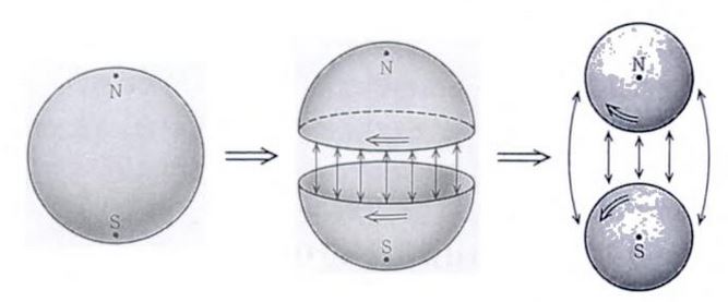
If we take the defining boundary inclusion itself as an attaching map, then we are gluing two -disks to each other along their common boundary . The result is the -sphere:
(graphics from Ueno-Shiga-Morita 95)
Example
A single cell attachment of a 0-cell, according to def. is the same as forming the disjoint union space with the point space :
In particular if we start with the empty topological space itself, then by attaching 0-cells we obtain a discrete topological space. To this then we may attach higher dimensional cells.
Definition
(attaching many cells at once)
If we have a set of attaching maps (as in def. ), all to the same space , we may think of these as one single continuous function out of the disjoint union space of their domain spheres
Then the result of attaching all the corresponding -cells to is the pushout of the corresponding disjoint union of boundary inclusions:
Apart from attaching a set of cells all at once to a fixed base space, we may “attach cells to cells” in that after forming a given cell attachment, then we further attach cells to the resulting attaching space, and ever so on:
Definition
Let be a topological space, then a topological relative cell complex of countable height based on is a continuous function
and a sequential diagram of topological space of the form
such that
-
each is exhibited as a cell attachment according to def. , hence presented by a pushout diagram of the form
-
is the union of all these cell attachments, and is the canonical inclusion; or stated more abstractly: the map is the inclusion of the first component of the diagram into its colimiting cocone :
If here is the empty space then the result is a map , which is equivalently just a space built form “attaching cells to nothing”. This is then called just a topological cell complex of countable hight.
Finally, a topological (relative) cell complex of countable hight is called a CW-complex if the -st cell attachment is entirely by -cells, hence exhibited specifically by a pushout of the following form:
A finite CW-complex is one which admits a presentation in which there are only finitely many attaching maps, and similarly a countable CW-complex is one which admits a presentation with countably many attaching maps.
Given a CW-complex, then is also called its -skeleton.
A cellular map between CW-complexes and is a continuous function such that .
Properties
Topological properties
Proposition
Every CW-complex is a locally contractible topological space.
Proposition
(CW-complexes are paracompact Hausdorff spaces)
Every CW-complex is a
-
a normal topological space, in particular a Hausdorff space,
Proposition
Every CW-complex is a compactly generated topological space.
Proof
Since a CW-complex is a colimit in Top over attachments of standard n-disks (its cells), by the characterization of colimits in (prop.) a subset of is open or closed precisely if its restriction to each cell is open or closed, respectively. Since the -disks are compact, this implies one direction: if a subset of intersected with all compact subsets is closed, then is closed.
For the converse direction, since a CW-complex is a Hausdorff space and since compact subspaces of Hausdorff spaces are closed, the intersection of a closed subset with a compact subset is closed.
In fact:
Proposition
Every CW-complex is a Delta-generated topological space.
Products of CW-complexes
If is an inclusion of CW-complexes, then the quotient is naturally itself a CW-complex, such that the quotient map is cellular.
If is a CW-complex and is a finite CW-complex, then the product topological space is naturally itself a CW-complex (see Brooke-Taylor 2017 for more and more generality, and see Prop. below).
For example the suspension of a CW-complex itself carries the structure of a CW-complex.
Similarly for pointed CW-complexes: the smash product of a pointed CW-complex with a finite pointed CW-complex is a pointed CW-complex. For example the reduced suspension of a pointed CW-complex is itself a CW-complex.
Proposition
(product preserves CW-complexes in compactly generated topological spaces)
For and CW-complexes with attaching maps and , then the k-ification of their product topological space (hence their Cartesian product in the category of compactly generated topological spaces) is again a CW-complex with attaching maps .
If either of the two CW-complexes is a locally compact topological space or if both are countable CW-complexes (have a countable set of cells) then
and so then the product topological space itself has CW-complex structure.
(e.g. Hatcher 2002, theorem A.6)
Up to homotopy equivalence
Theorem
Every CW complex is homotopy equivalent to (the realization of) a simplicial complex.
See Gray, Corollary 16.44 (p. 149) and Corollary 21.15 (p. 206). For more see at CW approximation.
Corollary
Every CW complex is homotopy equivalent to a space that admits a good open cover.
Theorem
If has the homotopy type of a CW complex and is a finite CW complex, then the mapping space with the compact-open topology has the homotopy type of a CW complex.
Subcomplexes
Proposition
For a CW complex, the inclusion of any subcomplex has an open neighbourhood in which is a deformation retract of . In particular such an inclusion is a good pair in the sense of relative homology.
For instance (Hatcher 2002, prop. A.5).
Remark
For the inclusion of a subcomplex into a CW complex, then the pair is often called a CW-pair. This appears notably in the axioms for generalized (Eilenberg-Steenrod) cohomology.
e.g. (AGP 02, def. 5.1.11)
Cellular approximation theorem
The cellular approximation theorem states that every continuous map between CW complexes (with chosen CW presentations) is homotopic to a cellular map (a map induced by a morphism of cell complexes).
This is the analogue for CW-complexes of the simplicial approximation theorem (sometimes also called lemma): that every continuous map between the geometric realizations of simplicial complexes is homotopic to a map induced by a map of simplicial complexes (after subdivision).
For more see at cellular approximation theorem.
Fibrations
Fibrations between CW-complexes also behave particularly well: a Serre fibration between CW-complexes is a Hurewicz fibration.
Singular homology
We discuss aspects of the singular homology Top Ab of CW-complexes. See also at cellular homology of CW-complexes.
Let be a CW-complex and write
for its filtered topological space-structure with the topological space obtained from by gluing on -cells. For write for the set of -cells of .
Proposition
The relative singular homology of the filtering degrees is
where denotes the free abelian group on the set of -cells.
The proof is spelled out at Relative singular homology - Of CW complexes.
Proposition
With we have
In particular if is a CW-complex of finite dimension of a CW-complex (the maximum degree of cells), then
Moreover, for the inclusion
is an isomorphism and for we have an isomorphism
This is mostly for instance in (Hatcher 2002, lemma 2.34 b),c)).
Proof
By the long exact sequence in relative homology, discussed at Relative homology – long exact sequences, we have an exact sequence
Now by prop. the leftmost and rightmost homology groups here vanish when and and hence exactness implies that
is an isomorphism for . This implies the first claims by induction on .
Finally for the last claim use that the above exact sequence gives
and hence that with the above the map is surjective.
Examples
Example
Any undirected graph (loops and/or multiple edges allowed) has a geometric realization as a 1-dimensional CW complex.
Example
The geometric realization of any simplicial set is a CW-complex (Milnor 57).
In particular, in the context of the homotopy hypothesis the Quillen equivalence between ∞-groupoids and nice topological spaces maps each ∞-groupoid to a CW-complex.
Example
The n-spheres have a standard CW-complex structure, with exactly 2-cells in each dimension, obtained inductively by attaching two -dimensional hemispheres to the -sphere regarded as the equator in the -sphere.
The infinite-dimensional sphere may be realized as the CW-complex which is the colimit over the resulting relative cell complex-inclusions . \end{example}
Example
Every projective space over the real numbers, complex numbers or quaternions has the structure of a CW-complex with a single cell i in each dimension , or , respectively. See at cell structure of K-projective space.
Example
(smooth manifolds) Every compact smooth manifold admits a smooth triangulation (by the triangulation theorem) and hence a CW-complex structure.
In the generality of manifolds with group actions see at G-CW complex – G-manifolds.
Every noncompact smooth manifold of dimension is homotopy equivalent to an -dimensional CW-complex. (Napier & Ramachandran).
Related concepts
examples of universal constructions of topological spaces:
References
The introduction of the term is contained in
- J. H. C. Whitehead, Combinatorial homotopy I , Bull. Amer. Math. Soc, 55, (1949), 213–245.
Basic textbook accounts:
-
Brayton Gray, Homotopy Theory: An Introduction to Algebraic Topology, Academic Press, New York (1975).
-
George Whitehead, chapter II of Elements of homotopy theory, 1978
-
Peter May, A Concise Course in Algebraic Topology, U. Chicago Press (1999)
-
Allen Hatcher, Algebraic Topology, Cambridge University Press 2002 (ISBN:9780521795401, webpage)
-
Allen Hatcher, Topology of cell complexes (pdf) in Algebraic Topology
-
Allen Hatcher, Vector bundles & K-theory (web)
-
Rudolf Fritsch, Renzo A. Piccinini, Cellular structures in topology, Cambridge studies in advanced mathematics Vol. 19, Cambridge University Press (1990). (doi:10.1017/CBO9780511983948, pdf)
-
Marcelo Aguilar, Samuel Gitler, Carlos Prieto, section 5.1 of Algebraic topology from a homotopical viewpoint, Springer (2002) (toc pdf)
Original articles include
-
John Milnor, On spaces having the homotopy type of a CW-complex, Trans. Amer. Math. Soc. 90 (2) (1959), 272-280.
-
John Milnor, The geometric realization of a semi-simplicial complex, Annals of Mathematics, 2nd Ser., 65, n. 2. (Mar., 1957), pp. 357-362; doi:10.2307/1969967, Semantic scholar pdf
On products of CW-complexes:
- Andrew Brooke-Taylor, Products of CW complexes – the full story, 2017 (pdf, pdf)
See also:
- Terrance Napier, Mohan Ramachandran, Elementary Construction of Exhausting Subsolutions of Elliptic Operators L’Enseignement Mathématique, t. 50 (2004), p. 367 - 389.
An inconclusive discussion here about what parts of the definition of a CW complex should be properties and what parts should be structure.
Last revised on February 5, 2024 at 03:12:51. See the history of this page for a list of all contributions to it.