nLab Grothendieck construction

Idea

In any context it is of interest to ask which kind of morphisms

$$\array{ E \\ \downarrow^{\mathrlap{p}} \\ C }$$

arise as pullbacks along a classifying morphism $S_p : C \to U$ to some universal object $U$ of some universal morphism

$$\array{ \hat U \\ \downarrow^{\mathrlap{p_{univ}}} \\ U } \,.$$

The Grothendieck construction describes this in the context of Cat: a morphism $p : E \to C$ of categories – i.e. a functor – is called a fibered category or Grothendieck fibration if it is encoded in a pseudofunctor/2-functor $S_p : C^{op} \to Cat$.

The reconstruction of $p$ from the pseudofunctor $S_p$ is the Grothendieck construction

$$\textstyle{\int} \;\; : \;\; Func(C^{op}, Cat) \to Cat/C$$

which is a fully faithful 2-functor from the 2-category of pseudofunctors $C^{op} \to Cat$ to the overcategory of Cat over $C$.

The essential image of this functor consists of Grothendieck fibrations and this establishes an equivalence of 2-categories

$$\textstyle{\int} \,\colon\, Func(C^{op}, Cat) \overset{\simeq}{\longrightarrow} Fib(C)$$

between 2-functors $C^{op} \to Cat$ and Grothendieck fibrations over $C$.

When restricted to pseudofunctors with values in Grpd $\subset$ Cat this identifies the Grothendieck fibrations in groupoids

$$\textstyle{\int} \;\colon\; Func(C^{op}, Grpd) \overset{\simeq}{\longrightarrow} FibGrpd(C) \,.$$

This equivalence notably allows one to discuss stacks equivalently as pseudofunctors or as groupoid fibrations (in each case satisfying a descent condition with respect to a Grothendieck topology on $C$).

The Grothendieck construction is one of the central aspects of category theory, together with the notions of universal constructions such as limit, adjunction and Kan extension. It is expected to have suitable analogs in all sufficiently good contexts of higher category theory. Notably there is an (∞,1)-Grothendieck construction in (∞,1)-category theory.

The Grothendieck construction can also be generalized beyond fibrations, to the correspondence between displayed categories and arbitrary categories over $C$.

Definition

Let Cat denote the 2-category of categories, functors and natural transformations.

In line with the philosophy of generalized universal bundles, consider the “universal Cat-bundle”

$$\begin{array}{c} Cat_{*,\ell} \\ \big\downarrow \\ Cat \mathrlap{\,,} \end{array}$$

namely the 2-category of “lax-pointed” categories, also known as the “lax slice” of Cat under the terminal category $\ast \,\in\, Cat$:

• Its objects are pointed categories (i.e. pairs $(A,a)$ where $A$ is a category and $a$ is an object of $A$)

• and its morphisms $(A,a) \to (B,b)$ are pairs $(f,\gamma)$, where $f \colon A\to B$ is a functor and $\gamma\colon f(a)\to b$ is a morphism in $B$.

• The projection $Cat_{*,\ell} \to Cat$ is the evident forgetful functor.

Now if $F \colon C \to Cat$ is a pseudofunctor from a category $C$ to $Cat$, then its Grothendieck construction is the (strict) 2-pullback $p \colon \int F \to C$ of $Cat_{*,\ell} \to Cat$ along $F$:

$$\array{ \int F &\longrightarrow& Cat_{*,\ell} \\ \mathllap{{}^{p}}\big\downarrow && \big\downarrow \\ C &\underset{F}{\longrightarrow}& Cat \mathrlap{\,.} }$$

This means that:

• the objects of $\int F$ are pairs $(c,a)$, where $c \in Obj(C)$ and $a \in Obj(F(c))$,

• and morphisms in $\int F$ are given by pairs $\big(c \overset{f}{\to} c',\, F(f)(a) \overset{\phi}{\to} a'\big)$. As systems of diagrams in Cat this looks as follows:

This construction extends to a 2-functor between bicategories

$$\textstyle{\int} \;\colon\; [C, Cat] \longrightarrow Cat/C$$

from pseudofunctors on $C$ to the overcategory of Cat over $C$.

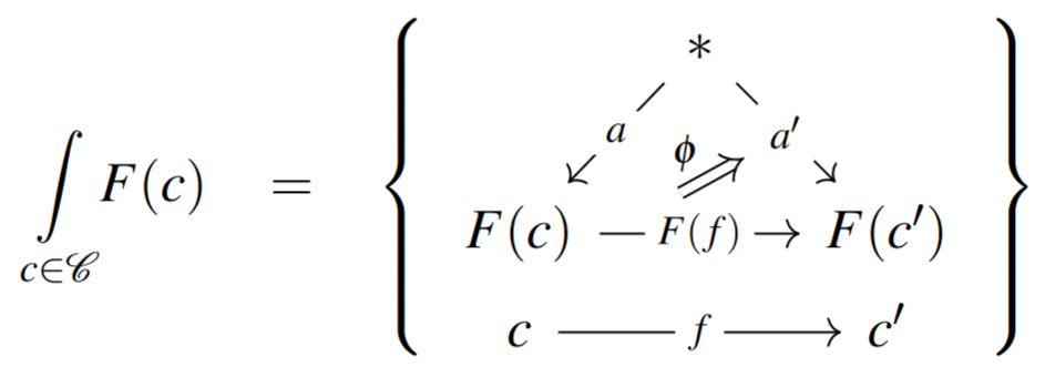
The more commonly described version of this construction works instead on contravariant pseudofunctors, i.e. pseudofunctors $C^{op}\to Cat$ from an opposite category. In this case we use instead the “universal $Cat$-cobundle” $(Cat_{*,c})^{op} \to Cat^{op}$, where $(Cat_{*,c})$ is the colax slice, whose objects are again pointed categories $(A,a)$, but whose morphisms $(A,a) \to (B,b)$ are pairs $(f,\gamma)$ where $f\colon A\to B$ and $\gamma\colon b \to f(a)$. Now the 2-pullback

$$\array{ \int F &\to& (Cat_{*,c})^{op} \\ {}^{\mathllap{p}}\downarrow && \downarrow \\ C &\stackrel{F}{\to}& Cat^{op} } \,.$$

constitutes a 2-functor

$$\textstyle{\int} \;\colon\; [C^{op},Cat] \longrightarrow Cat/C \,.$$

In this case,

• the objects of $\int F$ are again pairs $(c,a)$, where $c \in Obj(C)$ and $a \in Obj(F(c))$, but

• the morphisms in $\int F$ from $(c,a)$ to $(c',a')$ are pairs $\big(c \overset{f}{\to} c', a \overset{\phi}{\to} F(f)(a')\big)$:

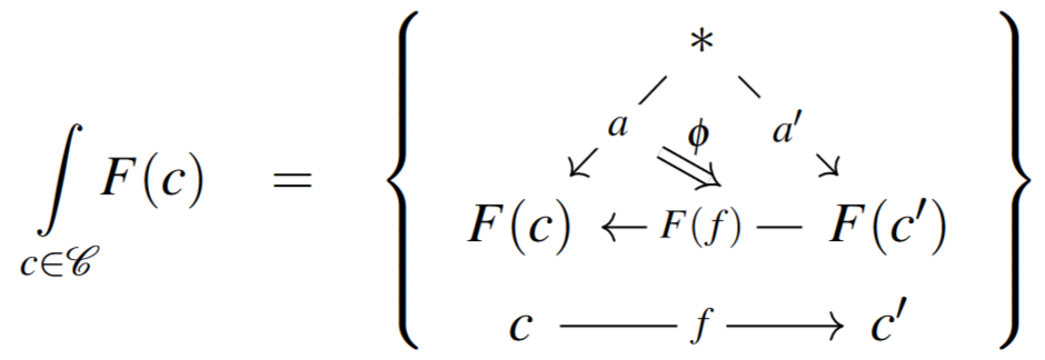
Note that this is not the same as the first (covariant) Grothendieck construction applied to $C^{op} \to Cat$, since, in that case, the morphisms between the objects of $C$ go in the opposite direction to one another.

Properties

(Co)Limits in a Grothendieck construction

We discuss existence and characterization of (co)limits in a Grothendieck construction.

Proposition

Given a pseudofunctor $F \colon C^{op} \to Cat$.

If

1. $C$ is complete.

2. $F(J)$ is complete for all $J \in C$.

3. $F(f) : F(J) \to F(K)$ preserves limits for all $f \colon K \to J$ in $C$.

then $\int F$ is complete.

Dually, if

1. $C$ is cocomplete.

2. $F(J)$ is cocomplete for all $J \in C$.

3. $F(f) : F(J) \to F(K)$ has a left adjoint for all $f : K \to J$ in $C$.

Then $\int F$ is cocomplete.

This proven in Tarlecki, Burstall & Goguen (1991), §3.1, 3.2.

The case of colimits is also described in Harpaz & Prasma (2015), Prop. 2.4.4:

Given a pseudofunctor

(1)$$\array{ \mathllap{ \mathbf{C} \,\colon\, \; } Base &\longrightarrow& Cat \\ \mathcal{X} &\mapsto& \mathbf{C}_{\mathcal{X}} \\ \Big\downarrow\mathrlap{{}^{f}} && \mathllap{^{f_!}}\Big\downarrow \dashv \Big\uparrow\mathrlap{{}^{f^\ast}} \\ \mathcal{Y} &\mapsto& \mathbf{C}_{\mathcal{Y}} }$$

such that

1. $Base$ is cocomplete

2. $\mathbf{C}_{\mathcal{X}}$ is cocomplete for each $\mathcal{X} \in Base$

then also the Grothendieck construction $\int_{\mathcal{X}} \mathbf{C}_{\mathcal{X}} \,\in\, Cat$ is cocomplete.

Explicitly, colimits in $\int_{\mathcal{X}} \mathbf{C}_{\mathcal{X}}$ are computed as follows:

Given a diagram in the Grothendieck construction

$$\mathscr{V}_{\mathcal{X}} \;\colon\; I \longrightarrow \textstyle{\int} \mathbf{C}_{(-)}$$

its underlying diagram in $Base$

$$\mathcal{X} \;\colon\; I \overset{ \mathscr{V}_{\mathcal{X}} }{\longrightarrow} \int \mathbf{C}_{(-)} \overset{\pi}{\longrightarrow} Base$$

has a colimit by assumption on $Base$, with coprojection morphisms to be denoted like this:

$$\mathcal{X}(i) \overset{\;\; q(i) \;\;}{\longrightarrow} \underset{\underset{j \in I}{\longrightarrow}}{\lim} \mathcal{X}(j) \,.$$

Now the idea is that the full colimit in $\int \mathbf{C}_{(-)}$ is obtained by

1. first pushing all morphisms $\phi \colon f_!\mathscr{V}(i) \to \mathscr{V}(j)$ in the diagram forward along the respective $q_j$

2. to hence obtain a diagram $q_! \mathscr{V}$ in $\mathbf{C}_{\underset{\longrightarrow}{\lim} \mathcal{X}}$

3. whose colimit $\underset{\longrightarrow}{\lim} q_! \mathscr{V}$ exists by assumption on $\mathbf{C}$

and then $\big(\underset{\longrightarrow}{\lim} q_! \mathscr{V}\big)_{\underset{\longrightarrow}{\lim}\mathcal{X}}$ is the desired colimit in $\int \mathbf{C}$

Example

(Cartesian product in Grothendick construction is external product on fiber categories )

Given a contravariant pseudofunctor

$$\array{ X \\ \Big\downarrow\mathrlap{{}^{f}} \\ Y } \;\;\;\;\;\mapsto\;\;\; \array{ \mathcal{C}_X \\ \Big\uparrow\mathrlap{{}^{f^\ast}} \\ \mathcal{C}_Y }$$

where the base category and all fiber categories $\mathcal{C}_{(-)}$ have Cartesian products and all base change maps $f^\ast$ preserve these products, then the Grothendieck construction $\int_X \mathcal{C}_X$ has cartesian products given on objects

$$\mathscr{V}_X \,\equiv\, \big( \mathscr{V} \,\in\, \mathcal{C}_X \big)$$

by the formula

(2)$$\mathscr{V}_X \times \mathscr{W}_Y \;\; \simeq \;\; \Big( \big(pr_X^\ast \mathscr{V}\big) \,\times\, \big(pr_Y^\ast \mathscr{W}\big) \Big)_{X \times Y} \,,$$

where we are denoting by

$$\array{ && X \times Y \\ & \mathllap{{}^{pr_X}}\swarrow && \searrow\mathrlap{{}^{pr_Y}} \\ X && && Y }$$

the product projection maps in the base category.

A product of the form (2) is known as an external tensor product, here the “external Cartesian product” on the fiber categories; see also this Proposition at free coproduct completion.

As an oplax colimit

The Grothendieck construction on $F : C \to Cat$ is equivalently the oplax colimit of $F$ (e.g Gepner-Haugseng-Nikolaus 15). That means that for each category $X$ there is an equivalence of categories

$$Lax(F, \Delta X) \simeq [{\textstyle \int} F, X]$$

that is natural in $X$, where $\Delta X$ is the constant functor with value $X$. (See oplax colimit for an explanation of why lax natural transformations appear in the definition of an oplax colimit.)

A lax natural transformation $\alpha$ from $F$ to $\Delta X$ is given by

• for each object $c$ of $C$, a functor $\alpha_c \colon F c \to X$, and
• for each morphism $m \colon c \to d$ in $C$, a natural transformation $\alpha_m \colon \alpha_c \Rightarrow \alpha_d \circ m_*$ (writing $m_* = F m$),

such that $\alpha_{1_c}$ is the isomorphism $F 1_c \cong 1_{F c}$ given by pseudofunctoriality of $F$, and that if $m \colon c \to d$, $n \colon d \to e$ is a composable pair in $C$, then $\alpha_{n m}$ is equal to the obvious pasting of $\alpha_m$ and $\alpha_n$.

We want to show that to each such lax transformation there corresponds an essentially unique functor $\int F \to X$. So firstly, given $\alpha$ as above, let $A$ be the functor that sends $x \in F c$ to $\alpha_c x$, and acts on arrows as

$$(m \colon c \to d, f \colon m_* x \to y) \quad \mapsto \quad \alpha_c x \overset{\alpha_m x}{\to} \alpha_d m_* x \overset{\alpha_d f}{\to} \alpha_d y$$

That $A$ is a functor follows from the coherence properties of $\alpha$ with respect to identities and composition in $C$.

Conversely, if $A \colon \int F \to X$ is a functor, we get a lax transformation $\alpha$ as follows:

• For each $c \in C$, $\alpha_c$ is the restriction of $A$ to the category $F c$, which is the subcategory of $\int F$ whose objects are those of $F c$ and whose morphisms are those with first component an identity morphism. This clearly makes $\alpha_c$ a functor.
• For each $m \colon c \to d$ in $C$, $\alpha_m$ has components $\alpha_c x \to \alpha_d m_* x$ given by $A$‘s value at the morphism $(m,1_{m_* x})$. This is a natural transformation because, if $k \colon x \to x'$ is a morphism in $F c$, then both sides of the naturality square are the value of $A$ at the morphism $(m, m_*k)$.

As one might expect, the coherence conditions on the resulting $\alpha$ follow from the functoriality of $A$.

It is then easy to check that these two mappings form a bijection between the objects of $Lax(F, \Delta X)$ and $[\int F, X]$.

As for the morphisms involved, the modifications between lax transformations and the natural transformations between functors, it is straightforward to show that these are in bijective correspondence too. Hence we have shown that the above equivalence holds.

By inspecting the above proof, it is easy to see that the lax transformation associated to a functor $\int F \to X$ is a pseudonatural transformation if and only if the functor inverts (i.e. sends to an isomorphism) each member of the class $S$ of morphisms of $\int F$ whose second component is an identity. (These are in fact the opcartesian morphisms with respect to the projection $\int F \to C$.) The localization $\int F[S^{-1}]$ is therefore the (weak) 2-colimit of $F$:

$$Ps(F, \Delta X) \simeq [{\textstyle \int} F, X]_{S^{-1}} \simeq [{\textstyle \int} F[S^{-1}], X]$$

This last result appears in SGA4 Exposé VI, Section 6.

Local smallness

In general, a (weighted) colimit of a large diagram of locally small categories need no longer be locally small. However, in the case of the oplax colimit, i.e. the Grothendieck construction, we have:

Theorem

If $F:C^{op}\to Cat$ is a pseudofunctor, $C$ is locally small, and each category $F(c)$ is locally small, then the Grothendieck construction $\int F$ is also locally small.

Proof

Recall that the morphisms in $\int F$ from $(c,a)$ to $(c',a')$ are pairs $(c \overset{f}{\to} c', a \overset{\alpha}{\to} F(f)(a'))$. Local smallness of $C$ means that there is only a set of such $f$‘s, and local smallness of $F(c)$ means that for each $f$ there is only a set of such $\alpha$’s.

For example, consider the canonical indexing? of a locally small category $A$, i.e. the pseudofunctor $Set^{op}\to Cat$ sending each set $X$ to the category $A^X$. This satisfies the conditions of the above theorem, so its Grothendieck construction, which is the category of families of objects of $A$, is locally small.

The equivalence between fibrations and pseudofunctors

One can characterize the image of the Grothendieck construction as consisting precisely of those objects in $Cat/C$ that are Grothendieck fibrations.

We recall the definition of the bicategory of Grothendieck fibrations and pseudofunctors and then state the main equivalence theorem.

The bicategory of pseudofunctors

A pseudofunctor from a 1-category $C$ to a 2-category (bicategory) $A$ is nothing but a (non-strict) 2-functor between bicategories, with the ordinary category regarded as a special bicategory.

We write $[C^{op}, A]$ for the 2-functor 2-category from the opposite category of $C$ to $A$ (the $op$ here is just convention):

• objects are pseudofunctors $F : C^{op} \to A$;

• morphisms are pseudonatural transformations;

• 2-morphism are modifications.

The bicategory of fibrations

Definition

A functor $p : E \to C$ is a Grothendieck fibration if for every object $e \in E$ and every morphism $f : c \to p(e)$ in $C$ there is a morphism $\hat f : \hat c \to e$ in $E$ that lifts $f$ in that $p(\hat f) = f$ and which is a Cartesian morphism.

A morphism of Grothendieck fibrations $F : (p : E \to C) \to (p' : E' \to C)$ is

• a functor $F : E \to E'$

• such that

  • $F$ sends Cartesian morphisms to Cartesian morphisms;

  • the diagram

    $$\array{ E &&\stackrel{F}{\to}&& E' \\ & {}_{\mathllap{p}}\searrow && \swarrow_{\mathrlap{p'}} \\ && C }$$

    in Cat commutes (strictly).

• a 2-morphism between morphism $\eta : F \to F'$ is a natural transformation of the underlying functors, that also makes the obvious diagram 2-commute, i.e. such that $p' \cdot \eta$ is trivial.

Compositions are those induced from the underlying functors and natural transformations.

This defines the 2-category of Grothendieck fibrations

$$Fib(C) \hookrightarrow Cat/C$$

over $C$, being a 2-subcategory of the overcategory of Cat over $C$.

Remark

Cartesian lifts are not required to be unique, but are automatically unique up to a unique vertical isomorphism connecting their domains.

Statement of the equivalence

Proposition

The Grothendieck construction factors through Grothendieck fibrations over $C$

$$\textstyle{\int} \;\colon\; [C^{op}, Cat] \longrightarrow Fib(C) \hookrightarrow Cat/C$$

and establishes an equivalence of bicategories

$$\textstyle{\int} \;\colon\; [C^{op}, Cat] \overset{\simeq}{\longrightarrow} Fib(C) \,.$$

In fact, it is more than that: it is an equivalence of strict 2-categories, in the sense of strict 2-category theory, i.e. an equivalence of $Cat$-enriched categories.

When restricted to pseudofunctors that factor through Grpd $\hookrightarrow Cat$ it factors through fibrations in groupoids

$$\textstyle{\int} \;\colon\; [C^{op}, Grpd] \longrightarrow Fib_{Grpd}(C) \hookrightarrow Cat/C$$

and establishes a similar equivalence

$$[C^{op}, Grpd] \simeq Fib_{Grpd}(C) \,.$$

Proof

This can be verified by straightforward albeit somewhat tedious checking. Details are spelled out in Johnstone (2002), B1.3. (The statement itself is theorem B1.3.6 there, all definitions and lemmas are on the pages before that.)

Model category version

There is refinement of the Grothendieck construction to model categories.

See at Grothendieck construction for model categories.

This model category incarnation of the Grothendieck construction generalizes to a model category presentation of the (∞,1)-Grothendieck construction.

Adjoints to the Grothendieck construction

The Grothendieck construction functor

$$\textstyle{\int} \;\colon\; [C^{op}, Cat] \longrightarrow Cat/C$$

has a left and a right adjoint functor.

Restricted to groupoid-valued functors and fibrations in groupoids, both of these exhibit the above equivalences as adjoint equivalences. The intuition for this is that all of the categorical structure of a groupoid is contained in the automorphism groups, so one does not need to look at functors $[C^{op}, GpdProf]$ in order to get all of the objects of $Gpd/C$.

Notice that much of the traditional literature discusses (just) the right adjoint.

The left adjoint

The left adjoint is the functor

$$L \colon (p : E \to C) \mapsto \big( (-)/p \colon C^{op} \to Cat \big)$$

that assigns to a functor $p$ the presheaf which sends $c \in C$ to the comma category $c/p$ with objects given by pairs $(e, c \to p(e))$ and morphisms by commutative triangles

$$\array{ && c && \\ & \swarrow && \searrow & \\ p(e_1) &&\to&& p(e_2) }$$

i.e.

$$L(E \stackrel{p}{\to}C) : c \mapsto c/p \,.$$

This functor may equivalently be expressed as follows.

In terms of a cone construction

For given $(E \stackrel{p}{\to} C)$ consider the (3,1)-pushout

$$\array{ E &\hookrightarrow& E^{\triangleright} \\ \downarrow^{\mathrlap{p}} &\swArrow& \downarrow \\ C &\to& K(p) }$$

of (2,1)-categories , where $K^{\triangleright}$ is $K$ with one terminal object $v$ adjoined (a join of categories). (Here $E$, $C$ and $E^{\triangleright}$ are 1-catgeories regarded trivially as $(2,1)$-categories and where $K(p)$ will in general be a (2,1)-category with nontrivial 2-morphisms).

Proposition

We have

$$c_{/p} \,\simeq\, Hom_{K(p)}(c,v) \,.$$

And hence the left adjoint to the Grothendieck construction may be realized as the assignment that sends $p \colon E \to C$ to the pseudofunctor

$$L(p) := Hom_{K(p)}(-, v) : C^{op} \to Cat \,.$$

Proof

It is convenient to compute the weak pushout by embedding the situation from Cat into the bigger context of (∞,1)-categories and using the model of that provided by sSet: the model structure for quasi-categories. This also facilitates the generalization of the argument from 1-categories to higher categories.

So consider equivalently the weak pushout diagram

$$\array{ N(E) &\hookrightarrow& N(E)^{\triangleright} \\ \downarrow^{\mathrlap{N(p)}} &\swArrow& \downarrow \\ N(C) &\to& N(K(p)) }$$

of quasi-categories, where $N(-)$ is the nerve operation and where $N(E)^{\triangleright} = N(E) \star *$ is the join of simplicial sets of $N(E)$ with the point.

By the general yoga of homotopy colimits (see there for details) we know that this $\infty$-pushout here may be computed as an ordinary pushout in the 1-category sSet if the pushout diagram $N(C) \leftarrow N(E) \to N(E)^{\triangleright}$ has the property that

• all three objects are cofibrant;

• at least one of the two morphisms is a cofibration

in the model structure for quasi-categories $sSet_{Joyal}$.

But this is trivially verified since the cofibrations in $sSet_{Joyal}$ are just the monomorphisms in sSet: the degreewise injective maps of simplicial sets. So every object in $sSet_{Joyal}$ is cofibrant and the inclusion $N(E) \hookrightarrow N(E)^{\triangleright}$ is a cofibration.

(The same conclusion would hold for the same simple reasons in the standard model structure on simplicial sets $sSet_{Quillen}$.)

From this it follows that simply because we passed from categories to their nerves, the computation of the weak pushout reduces to the computation of an ordinary pushout (one may think of passing to nerves as providing a cofibrant replacement: since in the nerve all composition of k-morphisms is “freed”, the nerve is a suitably “puffed up” version of a category that is suitable for computing $\infty$-pushouts).

So we are reduced to computing the ordinary pushout

$$\array{ N(E) &\hookrightarrow& N(E)^{\triangleright} \\ \downarrow^{\mathrlap{N(p)}} && \downarrow \\ N(C) &\to& Q }$$

in sSet. The fibrant replacement of $Q$ is then the nerve of the bicategory $K(p)$ that we are after.

As recalled at limits and colimits by example in the section limits in presheaf categories, colimits (and hence pushouts) in the presheaf-category sSet $= Func(\Delta^{op}, Set)$ are computed for each object $[n] \in \Delta$ as ordinary colimits in Set.

For $n=0$ we see that $Q_0$ is the collection of objects of $C$ and one additional vertex $v$:

$$Q_0 = N(C)_0 \coprod \{ v\} = p(Obj(E)) \coprod \{v \}$$

For $n=1$ similarly we find that $Q_1$ consists of the 1-cells in in $C$ and in addition of one 1-cell $e : c \to v$ for each $e \in Obj(E)$ with $p(e) = c$ (this 1-cell is really the terminal 1-cell $e \to v$ in $E^{\triangleright}$ but with its source re-interpreted as being $p(e) = c$ according to the identification of $Q_0$ as above). In the fibrant replacement of $Q$ the composite of original 1-cells $c_1 \to c_2$ and the new 1-cells $e : c_2 \to v$ will be freely added, so that the general 1-morphism $c_1 \to v$ will consist of a 1-morphism $c_1 \to c_2$ in $C$ together with a lift of $c_2$ to $E$. This is just as in the comma category $c/p$.

For $n=2$ we have in $Q_2$ the 2-cells in $C$ as well as one 2-cell

$$\array{ c_1 &&\to&& c_2 \\ & \searrow &{}^{(e_1 \to e_2)}\swArrow& \swarrow \\ && v }$$

for each 1-cell $(e_1 \to e_2)$ in $N(E)$ with $p(e_1 \to e_2)$ = $(c_1 \to c_2)$.

In particular this means that if $e_2: c_2 \to v$ is a morphism in $Q$ and $c_1 \to c_2$ is a morphism in $C$, then the composite $c_1 \to c_2 \to v$ in $Q$ is homotopic to any compatible direct morphism $c_1 \to v$ in $Q$.

This means that forming the fibrant replacement of $Q$ in $sSet_{Joyal}$ will not throw in superfluous 1-morphisms on top of those we already discussed in the previous paragraph…

Now furthermore…

This formulation of the Grothendieck construction as part of an adjunction

$$(L \dashv \textstyle{\int}) \;\colon\; Fib(C) \rightleftarrows [C^{op}, Cat]$$

with the left adjoint given by hom-objects in a pushout object as above is the starting point for its vertical categorification described at (∞,1)-Grothendieck construction.

The right adjoint

We also have an adjunction

$$(R \vdash \textstyle{\int}) \;\colon\; Fib(C) \rightleftarrows [C^{op}, Cat] \,,$$

where the right adjoint $R$ sends a Grothendieck fibration $F$ over $C$ to the presheaf

$$c \;\mapsto\; Hom(\textstyle{\int} y(c), F) \,,$$

where $\int y(c)$ is the Grothendieck construction applied to the representable presheaf of sets (hence discrete categories) on $c$ and $Hom$ denotes the category of morphisms between two Grothendieck fibrations.

Informally, an object of $R(F)(c)$ is given by a choice of a pullback along each morphism with codomain $c$, and these pullbacks must be functorial.

Behaviour under simplicial nerve

Proposition

For $F \colon \mathcal{D} \to Cat$ a functor, let

$${\vert N(F(-))\vert} \;\colon\; \mathcal{D} \overset{F}{\longrightarrow} Cat \stackrel{\vert N(-) \vert}{\to} Top$$

be its postcomposition with geometric realization of categories

Then we have a weak homotopy equivalence

$${\left\vert N\left(\textstyle{\int} F \right) \right\vert} \simeq hocolim {\vert N(F(-)) \vert}$$

exhibiting the homotopy colimit in Top over $\vert N(F (-)) \vert$ as the geometric realization of the Grothendieck construction $\int F$ of $F$.

This is due to (Thomason 79).

Further properties

Proposition

Given a contravariant pseudofunctor

$$\array{ \mathbf{D}^{op} &\overset{C_{(-)}}{\longrightarrow}& Cat \\ \mathbf{x} &\mapsto& C_{\mathbf{x}} \\ \Big\downarrow\mathrlap{{}^{\mathbf{f}}} && \Big\uparrow\mathrlap{{}^{\mathbf{f}^\ast}} \\ \mathbf{x}' &\mapsto& C_{\mathbf{x}'} }$$

and a pair of adjoint functors of the form

$$\mathcal{D} \underoverset {\underset{R}{\longleftarrow}} {\overset{L}{\longrightarrow}} {\;\; \bot \;\;} \mathbf{D}$$

then there is an induced adjunction between the Grothendieck constructions on $C_{(-)}$ and on $C_{L(-)}$ covering the given adjunction

$$\array{ \Bigg\{ \mathscr{V}_{x} \xrightarrow{ \phi_{f} } \mathscr{V}'_{x'} \;\displaystyle{\Bigg\vert}\; \array{ \mathscr{V} &\xrightarrow{ \phi }& L(f)^\ast \mathscr{V}' & \in C_{L(x)} \\ x &\xrightarrow{ f }& x' & \in \mathcal{D} } \Bigg\} \,\equiv & \Big( \underset {x \in \mathcal{D}} {\textstyle{\int}} C_{L(x)} \Big) & \underoverset {\underset{\widehat R}{\longleftarrow}} {\overset{\widehat L}{\longrightarrow}} {\;\; \bot \;\;} & \Big( \underset {\mathbf{x} \in \mathbf{D}} {\textstyle{\int}} C_{\mathbf{x}} \Big) & \equiv \, \Bigg\{ \mathscr{V}_{\mathbf{x}} \xrightarrow{ \phi_{\mathbf{f}} } \mathscr{V}'_{\mathbf{x}'} \;\displaystyle{\Bigg\vert}\; \array{ \mathscr{V} &\xrightarrow{ \phi }& \mathbf{f}^\ast \mathscr{V}' & \in C_{\mathbf{x}} \\ \mathbf{x} &\xrightarrow{ \mathbf{f} }& \mathbf{x}' & \in \mathbf{D} } \Bigg\} \\ & \Big\downarrow && \Big\downarrow \\ & \mathcal{D} & \underoverset {\underset{R}{\longleftarrow}} {\overset{L}{\longrightarrow}} {\;\; \bot \;\;} & \mathbf{D} }$$

where $\widehat L$ acts as $L$ on underlying morphisms and as the identity on components:

$$\array{ \mathscr{V}_{x} \\ \Big\downarrow\mathrlap{{}^{\phi_{f}}} \\ \mathscr{V}'_{x'} } \;\;\;\;\;\;\; \overset{\widehat L}{\mapsto} \;\;\;\;\; \array{ \mathscr{V}_{L(x)} \\ \Big\downarrow\mathrlap{{}^{\phi_{L(f)}}} \\ \mathscr{V}'_{L(x')} \mathrlap{\,,} }$$

while $\widehat R$ acts as $R$ on underlying morphisms and on components by base change along the adjunction unit $\epsilon_{\mathbf{x}} \colon L \circ R(\mathbf{x}) \to \mathbf{x}$:

$$\array{ \mathscr{V}_{\mathbf{x}} \\ \Big\downarrow\mathrlap{{}^{\phi_{\mathbf{f}}}} \\ \mathscr{V}'_{\mathbf{x}'} } \;\;\;\;\;\;\; \overset{\widehat R}{\mapsto} \;\;\;\;\; \array{ \big(\epsilon_{\mathbf{x}}^\ast \mathscr{V}\big)_{R(\mathbf{x})} \\ \Big\downarrow \mathrlap{{}^{ (\epsilon_\mathbf{x}^\ast \phi)_{ R(\mathbf{f}) } }} \\ \big(\epsilon_{\mathbf{x}'}^\ast \mathscr{V}\big)_{ R(\mathbf{x}')} }$$

and the adjunction counit is the identity morphism on components covering the underlying adjunction counit:

(3)$$\epsilon^{ \widehat{L} \dashv \widehat{R} }_{ \mathscr{V}_{\mathbf{x}} } \;\colon\; \widehat{L} \widehat{R} \big(\mathscr{V}_{\mathbf{x}}\big) = \Big( \big(\epsilon^{L \dashv R}_{\mathbf{x}}\big)^\ast \mathscr{V} \Big)_{ L R(\mathbf{x}) } \overset{ (id)_{\epsilon^{L \dashv R}_{\mathbf{x}}} }{\longrightarrow} \mathscr{V}_{\mathbf{x}}$$

Proof

First notice that $\widehat R$ is indeed well-defined in that we have a natural isomorphism on the right of

$$\epsilon_{\mathbf{x}}^\ast \mathscr{V} \xrightarrow{ \epsilon_{\mathbf{x}}^\ast \phi } \epsilon_{\mathbf{x}}^\ast \mathbf{f}^\ast \mathscr{V}' \simeq \big(L R(\mathbf{f})\big)^\ast \epsilon_{\mathbf{x}'}^\ast \mathscr{V}'$$

given by the contravariant pseudo-functoriality of $C_{(-)}$ applied to the commutativity of the naturality square of the adjunction counit:

$$\array{ L R(\mathbf{x}) &\overset{ L R(\mathbf{f}) }{\longrightarrow}& L R(\mathbf{x}') \\ \mathllap{{}^{ \epsilon_{\mathbf{x}} }} \Big\downarrow && \Big\downarrow \mathrlap{{}^{ \epsilon_{\mathbf{x}'} }} \\ \mathbf{x} &\underset{\;\; \mathbf{f} \;\;}{\longrightarrow}& \mathbf{x}' \mathrlap{\,.} }$$

Now if we write $f \colon x \to R(\mathbf{x}')$ for the $(L \dashv R)$-adjunct of a given $\mathbf{f} \colon L(x) \to \mathbf{x}'$ then we have natural bijections

$$\begin{array}{ll} \Big\{ \widehat L\big( \mathscr{V}_x \big) \xrightarrow{ \phi_{\mathbf{f}} } \mathscr{V}'_{\mathbf{x}'} \Big\} \\ \;\simeq\; \Big\{ \mathscr{V}_{L(x)} \xrightarrow{ \phi_{\mathbf{f}} } \mathscr{V}'_{\mathbf{x}'} \Big\} & \text{by def.} \\ \;\simeq\; \Big\{ \mathscr{V}_{x} \xrightarrow{ \phi_{f} } \big( \epsilon^\ast_{\mathbf{x}'} \mathscr{V}' \big)_{R(\mathbf{x}')} \Big\} & \text{see below} \\ \;\simeq\; \Big\{ \mathscr{V}_{x} \xrightarrow{ \phi_{f} } \widehat R \big( \mathscr{V}'_{\mathbf{x}'} \big) \Big\} & \text{by def.,} \end{array}$$

where the one step that is not a definition is on underlying morphisms the $(L \dashv R)$-hom-isomorphism

$$\begin{array}{ll} \Big\{ L(x) \xrightarrow{ \mathbf{f} } \mathbf{x}' \Big\} \;\simeq\; \Big\{ x \xrightarrow{ f } R(\mathbf{x}') \Big\} \end{array}$$

and on components the following natural bijection

$$\begin{array}{ll} \Big\{ \mathscr{V} \xrightarrow{ \phi } \mathbf{f}^\ast \mathscr{V}' \Big\} \\ \;\simeq\; \Big\{ \mathscr{V} \xrightarrow{ \phi } \big( \epsilon_{\mathbf{x}'} \,\circ\, L(f) \big)^\ast \mathscr{V}' \Big\} & \text{ formula for adjuncts } \\ \;\simeq\; \Big\{ \mathscr{V} \xrightarrow{ \phi } L(f)^\ast \big( \epsilon_{\mathbf{x}'}^\ast \mathscr{V}' \big) \Big\} & \text{ pseudo-functoriality, } \end{array}$$

where the first step uses the general formula $\mathbf{f} \,=\, \epsilon_{\mathbf{x}'} \circ L(f)$ (here) that expresses adjuncts in terms of the counit and the second step is the contravariant pseudo-functoriality of $C_{(-)}$.

This establishes a hom-isomorphism exhibiting adjoint functors $\widehat L \dashv \widehat R$. Moreover, the image of an identity morphism on $\widehat{R}(-)$ under this hom-isomorphism is the claimed counit (3).

Generalizations

$n = 0$

The analog of the Grothendieck construction one categorical dimension down is the category of elements of a presheaf.

$n = (\infty,0)$

The analog of the Grothendieck construction for ∞-groupoids is examined in detail in Heuts-Moerdijk 13.

The category of presheaves in groupoids is replaced by the model category of simplicial presheaves equipped with the projective model structure and the category of Grothendieck fibrations in groupoids is replaced by the model category of simplicial sets over the nerve of the source category, equipped with the contravariant model structure.

In this case there is not one, but two different functors that generalize the Grothendieck construction.

The first functor $h_!$ is a left adjoint, it implements the homotopy colimit using the diagonal of a bisimplicial set, and the second functor $r^*$ is a right adjoint, it uses the codiagonal (also known as the totalization) of a bisimplicial set. Both functors fit into adjunctions $h_!\dashv h^*$ and $r_!\dashv r^*$, where the other two adjoints can be seen as rectification functors: the right adjoint $h^*$ generalizes the cleavage construction, whereas the left adjoint $r_!$ generalizes the comma category construction above.

The two functors $h_!$ and $r^*$ become naturally weakly equivalent once we derive them, but they are not isomorphic. The functor $r^*$ restricted to the full subcategory of presheaves of groupoids recovers the nerve of the classical Grothendieck construction described above. The functor $h_!$ restricted to the same full subcategory does not even land in quasicategories, so it doesn’t give rise to a new construction in the classical case.

$n = (\infty,1)$

The analog of the Grothendieck construction for (∞,1)-categories is described at Cartesian fibration and at universal fibration of (∞,1)-categories.

The correspondence between $(\infty,1)$-categorical cartesian fibrations $E \to C$ and (∞,1)-presheaves $C \to (\infty,1)Cat^{op}$ is modeled by the Quillen equivalence between the model structure on marked simplicial over-sets and the projective global model structure on simplicial presheaves.

For more details see

• (∞,1)-Grothendieck construction

Normal lax functors into $Prof$

The Grothendieck construction can be generalized from pseudofunctors into $Cat$ to normal lax functors into Prof. Instead of fibrations over $C$, such normal lax functors correspond to arbitrary functors into $C$. See displayed category for more.

Warning on terminology

The term ‘Grothendieck Construction’ is applied in the literature to at least two very different constructions (and as Grothendieck introduced so many new ideas and constructions to mathematics, perhaps there are others!). One concerns the construction of a fibered category from a pseudofunctor and will be treated in more detail in the entry on Grothendieck fibration. The other refers to constructing the Grothendieck group is in the context of K-theory from isomorphism classes of vector bundles on a space by the introduction of formal inverses, ‘virtual bundles’. This constructs an Abelian group from the semi-group of isomorphism classes.

Examples

Example

(representable functor and slice categories)
A representable functor $C(-,X) \colon C^{op} \to Set \hookrightarrow Cat$ maps under the Grothendieck construction to the slice category $C/X$. The corresponding fibrations $C/X \to C$ are also called representable fibered categories.

Example

(slice categories and arrow category)
For $\mathcal{S}$ any category, let

$$\mathcal{S}_{(-)} \,\colon\, \mathcal{S} \longrightarrow Cat$$

be the pseudofunctor which sends

• an object $B \,\in\, \mathcal{S}$ to the slice category $\mathcal{S}_{/B}$,

• a morphism $f \colon B \to B'$ to the left base change functor $f_! \,\colon\, \mathcal{C}_{B} \to \mathcal{C}_{/B'}$ given by post-composition in $\mathcal{C}$.

The Grothendieck construction on this functor is the arrow category $\mathcal{S}^{I}$ of $\mathcal{S}$:

$$\mathcal{S}^{I} \;\;\; \simeq \;\;\; \textstyle{\int}_{B \in \mathcal{S}} \mathcal{S}_{/B} \mathrlap{\,.}$$

This follows readily by unwinding the definitions. In the refinement to the Grothendieck construction for model categories (here: slice model categories and model structures on functors) this equivalence is also considered for instance in Harpaz & Prasma (2015), above Cor. 6.1.2.

The correponding Grothendieck fibration is also known as the codomain fibration, a priori an opfibration.

But if $\mathcal{S}$ has all pullbacks, then there is also the contravariant pseudofunctor

$$\mathcal{S}_{(-)} \,\colon\, \mathcal{S}^{op} \longrightarrow Cat$$

which sends

• an object $B \,\in\, \mathcal{S}$ to the slice category $\mathcal{S}_{/B}$,

• a morphism $f \colon B \to B'$ to the base change functor $f^\ast \,\colon\, \mathcal{C}_{B'} \to \mathcal{C}_{/B}$ given by pullback in $\mathcal{C}$.

The corresponding (contravariant) Grothendieck construction is still the arrow category of $\mathcal{S}$, but now exhibited as a Grothendieck fibration (instead of or rather: in addition to being an opfibration) over $\mathcal{S}$. This is often the default meaning of the term codomain fibration.

In slight variation of Exp. :

Example

(pointed slice categories and retractive spaces)
Let $\mathcal{S}$ be a category with all pushouts and consider the pseudofunctor

$$\big(\mathcal{S}_{(-)}\big)^{\ast/} \,\colon\, \mathcal{S} \longrightarrow Cat$$

which sends

• an object $B \,\in\, \mathcal{S}$ to the category of pointed objects in the slice category $\mathcal{S}_{/B}$,

• a morphism $f \colon B \to B'$ to the functor $f_! \;\colon\; \big(\mathcal{S}_{/B}\big)^{\ast/} \to \big(\mathcal{S}_{/B'}\big)^{\ast/}$ which forms the pushout of retraction diagrams:

The corresponding Grothendieck construction is also known (at least when $\mathcal{S}$ is regarded as a category of “spaces”) as the category $\mathcal{S}_{\mathcal{R}}$ of “retractive spaces” in $\mathcal{S}$:

$$\mathcal{S}_{\mathcal{R}} \;\;\; \simeq \;\;\; \int_{B \in \mathcal{S}} \big( \mathcal{S}_{/\mathcal{B}} \big)^{\ast/} \,.$$

This follows readily from the definitions, but see also Braunack-Mayer (2021), Rem. 1.15; Hebestreit, Sagave & Schlichtkrull (2020), Lem. 2.14, where this is the basis of a model category-presentation of the tangent $\infty$-category of (the simplicial localization of) $\mathcal{S}$.

In alternative slight variation of Exp. :

Example

(abelianized slice categories and tangent category) For $\mathcal{S}$ a category with finite limits, let

$$Ab\big( \mathcal{S}_{/(-)} \big) \;\; \colon \;\; \mathcal{S}^{op} \longrightarrow Cat$$

be the contravariant pseudofunctor which sends

• any object $B \in \mathcal{S}$ to the category $Ab\big(\mathcal{S}_{/B}\big)$ of abelian group objects internal to the slice category $\mathcal{S}_{/B}$

• any morphism $f \colon B \to B'$ to the base change functor $f^\ast \colon Ab\big(\mathcal{S}_{/B'}\big) \to Ab\big(\mathcal{S}_{/B}\big)$ given by pullback in $\mathcal{C}$ (which preserves group objects).

The Grothendieck construction on this functor may be called the tangent category of $\mathcal{S}$.

Related concepts

• category of elements

• two-sided fibration

• indexed Grothendieck construction

• 2-Grothendieck construction

• (infinity,1)-Grothendieck construction

• Grothendieck construction for monoidal categories

References

The Grothendieck construction originates in:

• Alexander Grothendieck, §VI.8 of: Revêtements Étales et Groupe Fondamental - Séminaire de Géometrie Algébrique du Bois Marie 1960/61 (SGA 1) , LNM 224 Springer (1971) [updated version with comments by M. Raynaud: arxiv.0206203]

Review:

• Angelo Vistoli, §3.1.3 in: Grothendieck topologies, fibered categories and descent theory, in: Fundamental algebraic geometry – Grothendieck's FGA explained, Mathematical Surveys and Monographs 123, Amer. Math. Soc. (2005) 1-104 [ISBN:978-0-8218-4245-4, math.AG/0412512]

Further textbook accounts:

• Francis Borceux, Section 8.3 of: Handbook of Categorical Algebra, Vol. 2: Categories and Structures Encyclopedia of Mathematics and its Applications 50, Cambridge University Press (1994) (doi:10.1017/CBO9780511525865)

• Peter Johnstone, sections A1.1.7, B1.3.1 of: Sketches of an Elephant (2002)

• Garth Warner: Fibrations and Sheaves, EPrint Collection, University of Washington (2012) [hdl:1773/20977, pdf, pdf]

• Niles Johnson, Donald Yau, Chapter 10 of: 2-Dimensional Categories, Oxford University Press 2021 (arXiv:2002.06055, doi:10.1093/oso/9780198871378.001.0001)

Survey in the generality of enriched-, internal- and $\infty$-category theory (see also the enriched- and $\infty$-Grothendieck construction):

• Liang Ze Wong, The Grothendieck Construction in Enriched, Internal and ∞-Category Theory, PhD thesis, Univ. Washington (2019) [pdf, pdf]

The geometric realization of Grothendieck constructions has been analyzed in

• R. W. Thomason, Homotopy colimits in the category of small categories , Math. Proc. Cambridge Philos. Soc. 85 (1979), no. 1, 91109.

The left adjoint to the Grothendieck construction is discussed in §3.1.1 of

• Georges Maltsiniotis, La théorie de l’homotopie de Grothendieck

On limits and colimits in Grothendieck constructions:

• Andrzej Tarlecki, Rod M. Burstall, Joseph A. Goguen, Some fundamental algebraic tools for the semantics of computation: Part 3. Indexed categories, Theoretical Computer Science 91 2 (1991) 239-264 [doi:10.1016/0304-3975(91)90085-G]

The analog for simplicial sets instead of groupoids is discussed in

• Gijs Heuts, Ieke Moerdijk, Left fibrations and homotopy colimits (arXiv:1308.0704).

See also

• Grothendieck construction (Wikipedia)
• The Homotopy Theory of n-Fold Categories
• Inference System Integration via Logic Morphisms
• Category Theory for Computing Science

A model category presentation of the Grothendieck construction see at Grothendieck construction for model categories.

Discussion of the Grothendieck construction as a lax colimit includes (see also at (infinity,1)-Grothendieck construction)

• David Gepner, Rune Haugseng, Thomas Nikolaus, Lax colimits and free fibrations in $\infty$-categories (arXiv:1501.02161)

On the enriched Grothendieck construction:

• Jonathan Beardsley, Liang Ze Wong, The Enriched Grothendieck Construction, Advances in Mathematics, 344 (2019) 234-261 [arXiv:1804.03829, doi:10.1016/j.aim.2018.12.009]

• Jonathan Beardsley, Liang Ze Wong, The operadic nerve, relative nerve and the Grothendieck construction, Theory and Applications of Categories, 34 13 (2019) 349-374 [tac:34-13]

A monoidal version:

• Joe Moeller, Christina Vasilakopoulou, Monoidal Grothendieck Construction, 2019 (arXiv:1809.00727)