nLab
variational bicomplex

Idea

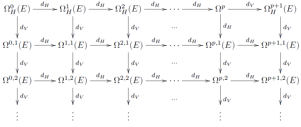
For $X$ a (spacetime) manifold and $E\to X$ a bundle (in physics called the field bundle) with jet bundle $j_{\mathrm{\infty }}E\to X$, the variarional bicomplex is essentially the de Rham complex of $j_{\mathrm{\infty }}E$ with differential forms bigraded by horizontal degree (with respect to $X$) and vertical degree (along the fibers of $j_{\mathrm{\infty }}E$)). Accordingly the differential decomposes as

$$D=d+\delta ,$$D = d + \delta \,,

where $d$ is the de Rham differential on $X$ and $\delta$ is the variational differential.

Much of classical mechanics and classical field theory on $X$ is formalized in terms of the variational bicomplex. For instance

• a field configuration is a section of $E$;

• a Lagrangian is an element $L\in {\Omega }^{n,0}(j_{\mathrm{\infty }}E)$;

• a local action functional is a map

  $$S:\Gamma (E)\to ℝ$$S : \Gamma(E) \to \mathbb{R}

  of the form

  $$S(\varphi )={\int }_{X}L(j_{\mathrm{\infty }}\varphi ),$$S(\phi) = \int_X L(j_\infty \phi) \,,

• the Euler-Lagrange equation is

  $$E(L):=\delta L\mathrm{mod}\mathrm{im}(d)=0$$E(L) := \delta L mod im(d) = 0

• the covariant phase space is the locus

  $$\{\varphi \in \Gamma (E)\mid E(L)(j_{\mathrm{\infty }}\varphi )=0\}$$\{ \phi \in \Gamma(E) | E(L)(j_\infty \phi) = 0 \}

• a conserved current is an element in ${\Omega }^{n-1,0}(j_{\mathrm{\infty }}E)$ that is $d$-closed on covariant phase space;

• a symmetry is a vertical vector field $v$ such that

  $$v(L)=0\mathrm{mod}\mathrm{im}(d)$$v(L) = 0 mod im(d)

• Noether's theorem asserts that every symmetry induces a conserved current.

Definition

Let $X$ be a smooth manifold and $p:E\to X$ some smooth bundle over $X$. Write $j_{\mathrm{\infty }}E\to X$ for the corresponding jet bundle.

The spaces of sections $\Gamma (E)$ and $\Gamma (j_{\mathrm{\infty }}E)$ canonically inherit a generalized smooth structure that makes them diffeological spaces: we have a pullback diagram of diffeological spaces

$$\begin{array}{ccc}\Gamma (E)& \to & *\\ \downarrow & & {\downarrow }^{\mathrm{id}}\\ [X,E]& \stackrel{p_{*}}{\to }& [X,X]\end{array}.$$\array{ \Gamma(E) &\to& * \\ \downarrow && \downarrow^{id} \\ [X,E] &\stackrel{p_*}{\to}& [X,X] } \,.

This induces the evaluation map

$$X\times \Gamma (E)\to E.$$X \times \Gamma(E) \to E \,.

and composed with the jet prolongation

$$j_{\mathrm{\infty }}:\Gamma (E)\to \Gamma (j_{\mathrm{\infty }}E)$$j_\infty : \Gamma(E) \to \Gamma(j_\infty E)

it yields a smooth map (homomorphism of diffeological spaces)

(1)$$e_{\mathrm{\infty }}:X\times \Gamma (E)\stackrel{(\mathrm{id},j_{\mathrm{\infty }})}{\to }X\times \Gamma (j_{\mathrm{\infty }}E)\stackrel{\mathrm{ev}}{\to }{j}_{\mathrm{\infty }}E.$$e_\infty : X \times \Gamma(E) \stackrel{(id,j_\infty)}{\to} X \times \Gamma(j_\infty E) \stackrel{ev}{\to} j_\infty E \,.

Write

$${\Omega }^{•,•}(X\times \Gamma (E))$$\Omega^{\bullet, \bullet}(X \times \Gamma(E))

for the cochain complex of smooth differential forms on the product $X\times \Gamma (E)$, bigraded with respect to the differentials on the two factors

$$D:=d+\delta ,$$D := d + \delta \,,

where the first $d=d_{\mathrm{dR}}$ is the de Rham differential on $X$.

Definition

The variational bicomplex of $E\to X$ is the sub–bi-complex of ${\Omega }^{•,•}(X\times \Gamma (E))$ that is the image of the pullback of forms along the map $e_{\mathrm{\infty }}$ (1):

$$e_{\mathrm{\infty }}^{*}:{\Omega }^{•}(j_{\mathrm{\infty }}E)\to {\Omega }^{•}(X\times \Gamma (E)).$$e_\infty^* : \Omega^{\bullet}(j_\infty E) \to \Omega^\bullet(X \times \Gamma(E)) \,.

We write

$${\Omega }_{\mathrm{loc}}^{•,•}:=\mathrm{im}(e_{\mathrm{\infty }}^{*})$$\Omega^{\bullet, \bullet}_{loc} := im (e_\infty^*)

and speak of the bicomplex of local forms on sections on $E$.

The bicomplex structure on ${\Omega }_{\mathrm{loc}}^{•,•}$ is attributed in (Olver) to (Takens). The above formulation as the image of the evident bicomplex of forms on $X\times \Gamma (E)$ is due to (Zuckerman, p. 5).

Properties

The fundamental variational formula

Definition

A source form is an element $\alpha$ in ${\Omega }_{\mathrm{loc}}^{n,1}$ such that

$${\alpha }_{\varphi }(\delta \varphi )$$\alpha_\phi(\delta \phi)

depends only on the 0-jet of $\delta \varphi$.

Proposition

Let $L\in {\Omega }_{\mathrm{loc}}^{n,0}$.

Then there is a unique source form $E(L)$ such that

$$\delta L=E(L)+d\Theta .$$\delta L = E(L) + d \Theta \,.

Moreover

• $E(L)$ is independent of changes of $L$ by $d$-exact terms:

  $$E(L)=E(L+dK).$$E(L) = E(L + d K) \,.

• $\Theta$ is unique up to $d$-exact terms.

This is (Zuckerman, theorem 3).

Here $E$ is the Euler-Lagrange operator .

Definition

Write

$$\Omega =\delta \Theta .$$\Omega = \delta \Theta \,.

Remark

By prop. 1 have

$$d\Omega =\delta E(L).$$d \Omega = \delta E(L) \,.

Proposition

$\delta E$ vanishes when restricted to vertical tangent vectors based in covariant phase space (but not necessarily tangential to it).

$$\delta E(L){\mid }_{T_{E(L)=0}\Gamma (E)}=0.$$\delta E(L) |_{T_{E(L) = 0} \Gamma(E)} = 0 \,.

This is (Zuckerman, lemma 8).

Presymplectic covariant phase space

Corollary

The form $\Omega$ is a conserved current.

Proof

By remark 1 and prop. 2.

Definition

For $\Sigma \subset X$ a compact closed submanifold of dimension $n-1$, one says that

$$\omega :={\int }_{\Sigma }\Omega \in {\Omega }_{\mathrm{loc}}^{0,2}$$\omega := \int_\Sigma \Omega \in \Omega^{0,2}_{loc}

is the presymplectic structure on covariant phase space relative to $\Sigma$.

Proposition

The 2-form $\omega$ is indeed closed

$$\delta \omega =0$$\delta \omega = 0

and in fact exact:

$$\theta :={\int }_{\Sigma }\Theta$$\theta := \int_\Sigma \Theta

is its presymplectic potential .

$$\delta \theta =\omega .$$\delta \theta = \omega \,.

Symmetries

Let $L\in {\Omega }_{\mathrm{loc}}^{n,0}$.

Definition

A vertical vector fields $v\in T_{v}E\subset T_v{j}_{\mathrm{\infty }}E$ is a symmetry if

$$v(L)=0\mathrm{mod}\mathrm{im}(d).$$v(L) = 0 mod im(d) \,.

Proposition

The presymplectic form $\omega$ from def. 4 is degenerate on symmetries.

This appears as (Zuckerman, theorem 13).

References

The variational bicomplex was introduced independently in

• W.M. Tulczyjew, The Euler-Lagrange resolution , in Lecture Notes in Mathematics 836 22–48 (Springer-Verlag, New York 1980).

• A.M. Vinogradov, A spectral sequence associated with a non-linear differential equation, and the algebro-geometric foundations of Lagrangian field theory with constraints , Sov. Math. Dokl. 19 (1978) 144–148.

• A.M. Vinogradov, The $C$-spectral sequence, Lagrangian formalism and conservation laws I, II, J. Math. Anal. Appl. 100 (1984) 1–129.

Also

• F. Takens, A global version of the inverse problem of the calculus of variations J. Diff. Geom. 14 (1979) 543-562

An textbook account is in section 5.4 of

• Peter Olver, Applications of Lie groups to differential equations, Springer Graduate Texts in Mathematics 107 (1986)

An invariant version (under group action) is in

• Irina A. Kogan, Peter J. Olver, The invariant variational bicomplex, pdf

An early discussion with application to covariant phase spaces and their presymplectic structure is in

• G. J. Zuckerman, Action principles and global geometry , in Mathematical Aspects of String Theory, S. T. Yau (Ed.), World Scientific, Singapore, 1987, pp. 259€284. (pdf)

An introduction is in

• Ian Anderson, Introduction to the variational bicomplex in Mathematical aspects of classical field theory, Contemp. Math. 132 (1992) 51–73, gBooks

• Ian Anderson, The variational bicomplex, Utah State University (1989) (pdf) (textbook account)

• Victor Kac, An explicit construction of the complex of variational calculus and Lie conformal algebra cohomology, talk at Algebraic Lie Theory, Newton Institute 2009, video

A generalization to multisymplectic geometry is discussed in

• Thomas Bridges, Peter Hydon, Jeffrey Lawson, Multisymplectic structures and the variational bicomplex (pdf)