Schreiber Modern Physics formalized in Modal Homotopy Type Theory
-
Modern Physics formalized in Modal Homotopy Type Theory,
(pdf)
expanded notes for a talk at
What are Suitable Criteria for a Foundation of Mathematics?
FOMUS – Foundations of Mathematics, July 2016
more (video-)exposition at: Perì Pantheōrías
Abstract. Where plain homotopy type theory provides a formal concept-logic, adding adjoint modal operators to it (Shulman 12, Schreiber-Shulman 14, Licata-Shulman 15, Shulman 15) serves to encode determinations of further qualities. Following (Lawvere 9x-0x), these categories of being naturally organize themselves in a progressive system of oppositions and resolutions which the inclined philosopher might enjoy to compare to the informal “Science of Logic”. This formal substance of modal homotopy type theory subsumes modal predicate logic but is immensely more expressive. The talk surveys how (Schreiber 13) externalizing this idea into natural models gives rise to the modern mathematics of space in higher/derived geometry and to modern physics of local prequantum field theory in supergravity/string theory.
For full technical details glossed over in the following see:
Contents
- Introduction
- Expanded talk notes
- Subjectivity
- The method (absolute Idea)
- Objective Logic
- Objectivity
- Classical mechanics (Mechanism)
- Quantum mechanics ((quantum-)Chemism)
- Boundary conditions (Teleology)
- The idea
- Maurer-Cartan forms
- Differential cohomology
- WZW terms
- -Manifolds
- Frame bundles
- -Structure
- Definite forms
- Nature
- Acknowledgements
- References
Introduction
We survey axioms for a system of modal operators that may naturally be added to homotopy type theory; and we survey how these induce a synthetic formalizaton of differential cohomology, higher differential geometry and of key structures in fundamental physics, notably Einstein-Cartan higher gauge prequantum field theory (dcct).
Formalization. The following is written in the pseudocode formerly known as mathematics. Parts of this have been fully formalized in computer-verified code (Shulman), the rest is in a form that should lend itself to such full formalization.
Synthetic axioms. Here synthetic axiomatics is meant in contrast with the following analytic axiomatics: The restriction of homotopy type theory to homotopy 0-types (“h-sets”) is a constructive set theory. A traditional assumption is that in principle and with enough patience it is possible to fullly formalize all rigorous mathematics in set theory, and with a little bit of extra care added also in constructive set theory. This way one could imagine to formalize, in principle and with much patience, first standard simplicial homotopy theory within the h-sets, then formalize the homotopy theory of simplicial presheaves, hence of infinity-stacks, to obtain a full formalization of homotopy toposes, then impose axioms on these to formalize the particular examples of, say, smooth infinity-groupoids, formal smooth infinity-groupoids and super formal smooth infinity-groupoids that are the necessary backdrop for, finally, formalizing modern physics.
While this program already sounds hardly tractable in practice, its practical usefulness is arguably even more remote. One is reminded of the fully formal proof of which in the Principia Mathematica takes 300 pages. Nobody ever did or will ever do any useful mathmatics (as opposed to metamathematics) based on this.
But in both cases type theory and homotopy type theory, respectively, comes to the rescue. In type theory the proof of is as trivial as it should be, thanks to the natural concept of inductive types. Similarly, in homotopy type theory the concept of infinity-stacks is already built in: every type in homotopy type theory has the generic interpretation of an infinity-stack. Instead of throwing that away by restricting to homotopy 0-types (whose interpretation is as mere sheaves of sets) and then tediously analytically rebuilding the informaltion thus lost, it is clearly advisable to retain that structure and make use of it synthetically. This is what we do below.
Modern physics. Our axioms owe a lot to William Lawvere, who had long ago suggested ( Toposes of laws of motion ) that some suitable elementary axioms imposed on toposes should provide a good context for formalization of physics. Lawvere’s axioms of synthetic differential geometry allow to formalize differential equations and hence much of classical field theory (his motivation is drawn from continuum mechanics). However, modern physics is considerably richer than that, being based on local higher gauge quantum field theory, including fermions, hence supergeometry, and including boundary conditions such as branes in string theory. Our axioms serve to formalize considerable chunks of this, and they do so naturally in that these structures follow from just a few lines of universal constructions involving the axioms.
Metaphysics. The following indulges in idealistic jargon of “subjective and objective logic”, following (Lawvere 92, Lawvere-Rosebrugh 03, section C.1). This is meant as a suggestion for a kind of pre-mathematical meaning explanation of the axioms. Dies zu wissen ist nicht not.
Expanded talk notes
Subjectivity
Concept
We use the Laws of Type:
Homotopy type theory as such (UFP 13) is a logic of types, of (mathematical) concepts (Martin-Löf 73, 1.1, Ladyman&Presnel 14). (References which recall that the modern “type” is a contraction of “type of mathematical concepts” include for instance also (Sale 77, p. 6).
With the univalence axiom for weakly Tarskian type universes included – which says that this essence appears properly reflected within itself – then its interpretation via categorical semantics is in elementary homotopy toposes (Shulman 12a, Shulman 12b, Shulman 14). These are the models of homotopy type theory. Conversely, homotopy type theory is the internal language of homotopy toposes, hence the latter are its “externalization”. This way homotopy type theory overlaps much with (higher) categorical logic. See at relation between type theory and category theory for more background on this.
Accordingly, since it is more immediately readable, we display mostly categorical expressions in the following, instead of the pure type theoretic syntax.
Judgement
The earliest formulation of a logic of concepts is arguably Aristotle's logic, which famously meant to reason about the relation of concepts such as “human” and “mortal”. We consider now a natural formalization of at least the core intent of Aristotle’s logic in dependent homotopy type theory.
Formalizations of Aristotle’s logic in categorical logic or type theory has previously been proposed in (LaPalmeReyes-Macnamara-Reyes 94, 2.3) and in (Pagnan 10, def. 3.1). The formalization below agrees with these proposal in the identification of the Aristotlean judgement “All are ” with the type-theoretic judgement “”, and with the identification of syllogisms with composition of fuch function terms.
All are .
If is a concept, a type, then a judgement
says that is an instance of the concept , or that is a term of type .
For instance if is the concept of natural numbers, then the judgement says that is a natural number. Clearly here the “concept” may just as well be thought of as the set of all its instances.
Given concepts/types and , there is the concept of maps between them, the function type . In the categorical semantics this is the internal hom.
The judgement that there is a function, hence an instance of the concept of functions
says that is a rule that takes instances/terms of to instances/terms of . At least if this is a monomorphism (so that the corresponding is a proposition) then this says in words that witnesses the fact that
All instances of are instances of .
or for short just
All are
hence that if is das Allgemeine (general, universal) concept then is das Besondere (special, particular) concept.
This formalization of Aristotle’s “All are ” in categiorical logic/type has been proposed in (LaPalmeReyes-Macnamara-Reyes 94, 2.3), where it is attributed to William Lawvere, and in (Pagnan 10, def. 3.1).
Notice that the choice of here is an important part of the formalization which is missing in Aristotle’s informal logic and causing ambiguity there.
For instance all natural numbers are real numbers, but there are many inequivalent subgroup inclusions realizing this. For the purposes of prequantum field theory these choices correspond to the choice of Planck's constant (see the discussion there).
Similarly, once we have that the informal “All are .” is formalized by a map of types, we see further refinement of the ancient logical notion.
First, the meaning of , may depend on some context . Leaving that implicit is arguably the greatest source of ambiguity in Aristotle’s logic. But it is easily fixed while staying true to the original intention: in general and are to be taken as -dependent types. Then the intended meaning of All are . is expressed by the dependent product over the function type formed in context
Second, if is not a monomorphism it still expresses the fact that for every instance of there is a corresponding instance of . Hence in general, we should further specify if is an n-truncated morphism. This is a general phenomenon in passing to higher homotopy types: the (epi, mono) factorization system on homotopy 0-types refines to a tower of (n-epi, n-mono) factorization systems for all natural numbers .
Individual is .
There is the unit type
of which there is a unique instance, das Einzelne (individual). As a concept, this may be regarded as the concept of pure being: since any two instances of the concept just purely are, there is no distinction and hence there is a unique instance.
Hence a function of the form is equivalently an instance/term of . In words this says that
The individual is an instance of the general concept .
of for short just
Individual is .
There is the identity type , which expresses the concept that is equivalent to itself.
The single introduction rule for identity types gives for all the statement that there is indeed an instance of this concept
The categorical semantics of is the loop space object , which is canonically a pointed object via the constant loop .
Under composition of loops, this object canonically carries the structure of an infinity-group.
Proposition
In any homotopy topos , the operation of forming loop space objects constitutes an equivalence of (infinity,1)-categories
between infinity-groups in and pointed connected objects in .
The inverse equivalence is called delooping. See at looping and delooping for more.
Now in homotopy type theory and in elementary (infinity,1)-toposes, the definition of infinity-groups as grouplike A-infinity algebras is not available, since the latter is not a finitary concept. But by prop. the concept also has a simple finitary equivalent incarnation, which is available in homotopy type theory: we may identify an infinity-group with its pointed connected delooping type .
Indeed, this is most useful: homotopy type theory in the context of is the infinity-representation theory of :
representation theory and equivariant cohomology in terms of (∞,1)-topos theory/homotopy type theory (FSS 12 I, exmp. 4.4):
Some is .
In order to formalize judgements of intersection of concepts of the form
Some is .
it is necessry to specify a context. Regard both and as dependent types witnessed by display maps
to a common context . Then the product type in context, hence, in the categorical semantics, the homotopy fiber product
is the type whose terms are the “some” instances of which are also instances of , and vice versa. Indeed, the fiber product canonically sits in the homotopy pullback diagram
and if we read as “some ” then according to the previous paragraph the top morphism expresses that “all of these particular (but not necessarily all of itself) are ”.
Example
(principal infinity-bundles as judgements)
Specifically if here is pointed via a map from , and connected, hence equivalently the delooping of its infinity-group of loops, then (writing now for ) a map of types
may be thought of as a cocycle on with coefficients in , representing a class in the nonabelian cohomology of . See at cohomology for more on this general concept of cohomology.
In this case the homotopy fiber of is the -principal infinity-bundle classified by , fitting into the homotopy pullback square.
Via the above translation this is an Aristotlean judgement of the form “Some are ” in the context of .
Summary
In summary we have that basic judgements in Aristotle’s logic, when some implicit assumptions are made explicit and the broad intention is retained, are naturally taken to be formalized in type theory as combinations of a type former and a judgement asserting a term of that type, as follows.
| Aristotle's logic | formal syntax | type theory |
|---|---|---|
| concept | type | |
| judgement | typing judgement | |
| All are . | function type | |
| Some is . | product type | |
| Individual is . | . | unit type/global element |
Deduction
The figure
Functions may be composed. Given and , then their composite is a function . In type theory this is an example of natural deduction (cut elimination), in words this is a syllogism
All are .
Individual is .
Hence
Individual is .
The figure
Analogously, the categorical semantics for
Some is .
All is .
Hence
Some is .
(all in some context ) is given by the horizontal composite in diagrams of the form
The method (absolute Idea)
What is not present in such bare homotopy type theory is determination of further qualities of types. For instance for synthetically formalizing physics one needs that types have topological and moreover differential geometric qualities to them. Some externalizations of homotopy type theory exhibit these, others do not. We now consider adding axioms to homotopy type theory that narrow it in on those models that do exhibit further quality in addition to the pure being of types.
Moments
A general abstract way to express a kind of quality carried by types is to posit a projection operation that projects out the moment of pure such quality.
For instance for formalizing realistic physics one needs to determine bosonic and fermionic moments (we come to this below), and one way of doing so is by considering a projection operation that projects every space of fields to its purely bosonic body (lemma below).
Generally, for a type, then is to be the result of projecting out some pure quality of . This being a projection means that . For this to be constructive, we need to specify a specific comparison map that gives this equivalence. Hence we say a moment projection is an operation on the type system together with natural functions such that is an equivalence .
In categorical semantics this means essentially that is an idempotent monad on the type system .
Alternatively we may ask for a comparison map the other way around, , such that is an equivalence. In categorical semantics this means essentially that is an idempotent comonad.
Definition
A moment on (or in) a type system is
or
- an idempotent comonad .
Given a moment, we write
for the inclusion of its image, which we think of as the collection of those types that exhibit the moment purely (conversely these define the kind of moment as whatever quality it is that they all exhibit purely).
Remark
This is a language construct natural and familiar also from the point of view of computational trinitarianism, see at monad (in computer science).
Further, it makes sense to refer to moments also as modal operators or just modalities for short, and speak of type theory equipped with such operators as modal type theory, a type-theoretic refinement of modal logic. In this language the types in are the -_modal types.
Remark
A moment or may be thought of as encoding a concept of similarity: as the operator projects out some details of the quality of a type and only retains some pure moment, it coarse-grains the nature of a type to some extent. Hence two types and may be different but “similar with respect to -quality” if their images under are equivalent:
(where on the right we have an identity type of the type universe).
Examples are made explicit below as ex. and ex..
Proposition
The category is equivalently the Eilenberg-Moore category of .
This is a standard fact in category theory, see at idempotent monad – Algebras.
Remark
Prop. means that we may naturally make sense of “pure qualtity” also for (co-)monads that are not idempotent, the pure types should be taken to be the “algebras” over the monad.
A single moment or may be interpreted as most anything, since it is not further determined yet. One now observes that there is an intrinsic, self-propelling way to further determine such abstract moments, by asking for their opposite and for their negative moments.
Opposites
Definition
(unity of opposites)
The opposite of a moment , def. is, if it exists, another moment in adjunction with it,
-
either left adjoint to and such that there is an adjoint triple
which we denote by
-
or right adjoint to it with
which we denote by
(We always display adjoint functors with the left adjoint on top and its right adjoint beneath.)
We say that the adjunction itself is the unity of opposites, and we indicate this by labels as in
Remark
In categorical semantics an opposition of moments, def. ,
-
of the form defines an essential subtopos, the image of . This is also called a level of a topos.
-
of the form defines a bireflective subcategory (in the sense of: reflective and coreflective subcategory).
It is fairly familiar from the practice of category theory that adjunctions express oppositions. The following example is drawn from arithmetic and is meant to illustrate this in a familar context, but the actual examples that we will be concerned with are more fundamental.
Example
Consider the two inclusions of the even and the odd integers, i.e. the maps and , respectively.
Both are adjoint to the operation of forming the of the result of dividing by two, this is right adjoint to the inclusion of even numbers, and left adjoint to the inclusion of odd numbers.
This has been considered in (Lawvere 00)
Example
Consider the inclusion of the integers into the real numbers, both regarded linear orders. This inclusion has a left adjoint given by and a right adjoint given by . The composite is an idempotent monad and the composite is an idempotent comonad on . Both express a moment of integrality in an real number, but in opposite ways, each real number sits in between its floor and celling
This example highlights that:
Remark
There is an opposition between the two kinds of opposition here:
-
– Here are two different opposite “pure moments” .
-
– Here is only one pure moment, but two opposite ways of projecting onto it.
Determinate negation
If is a pure moment found inside , then it makes to ask for its complement moment or its negative
Definition
The negative of a comonadic moment is what remains after taking away the piece of pure -quality, hence is the cofiber of the counit map:
The intuitive meaning suggests to ask whether this kind of negation of determinations is faithful in that there is no -moment left in the negative , hence whether
In general there is no reason for this to be the case. But if also has an opposite in the sense of def. , then one of the two opposite moments is left adjoint, hence preserves cofibers, and then a little more may be said.
Consider the case of an opposition of the form . In view of remark then both and express the same pure moment, just opposite ways of projecting onto it. Therefore in this situation it makes sense to alternatively ask that there is no -moment left in the .
Definition
Given a unity of opposite moments , def. , we say this has determinate negation if and both restrict to 0-type and such that there
-
;
-
is epi.
Proposition
For an opposition with determinate negation, def. , then on 0-types there is no -moment left in the negative of -moment:
Proof
Given that , being a left adjoint, preserves colimits, hence cofibers, the first condition in def. gives that
Now the second condition and the fact that epiness is preserved by pushout say that this result receives an epimorphism from the terminal object. But this forces it to be the terminal obect itself.
The proof of prop. depends crucially on the restriction to 0-types. At the other extreme, on stable types the intuition that -moment is complementary to -moment is verified in the following sense:
Proposition
For opposite moments of the form , def. , then for stable types the hexagons
are homotopy exact in that
-
both squares are homotopy Cartesian, hence are fracture squares;
-
the boundary sequences are long homotopy fiber sequences.
In particular every stable type is the fibered direct sum of its pure -moment and its pure -moment:
In this form this has been highlighted in (Bunke-Nikolaus-Völkl 13) in the context of our prop. below. See at differential hexagon for the proof.
Note that in the diagram we have also referred to the negative of a monadic moment, . We define this as follows:
Accidence
Definition
Say that a moment , is exhibited by a type if is equivalently -homotopy localization
This implies in particular that .
Progression
We have seen how to formalize determination of qualities of types together with their opposite and their negative determination. But so far these determinations are abstract in that when interpreting them in models they could come out as all kinds of very different-natured (co-)monads. What is missing is something that bases these determinations on a concrete ground with respect to which they would gain actual meaning.
Indeed, there are natural ways in which determinations of qualities may progress from given ones to further ones: on the one hand a given unity of oppositions may itself have an opposite and hence exhibit a higher order “opposition of oppositions”, on the other hand a given unity of oppositions may be “resolved” inside one new quality, which then in turn may have its own opposite and negative in turn, and so on.
Progression I: Higher order opposition
Given a concrete particular moment (i.e. an interpretation of the moment in categorical semantics), then adjoints to it are a property of the moment, not a choice to made. Abstractly we may specify that moments proceed to further moments this way by positing further adjoints.
Definition
(opposition of unities of oppositions)
Given one opposition , we say that on opposition of oppositions is a further left adjoint , which we may think of as constituting a system of adjoints of this form:
(Indeed, an adjoint triple is equivalently an adjunction of adjunctions, see here).
In principle this may go on, but in models one finds that there are essentially no examples with a fourth adjoint that do not degenerate to the ambidextrous situation where .
This shows further how oppositions serve to further determine moments: while a bare -operator has all kinds of unrelated interpretations in models, asking it to be in opposition with a -moment considerably constrains its possible interpretations, further asking it to participate in an opposition-of-oppositions constraints it much more still, and asking for yet one more opposition tends to overconstrain it such as to degenerate.
Progression II: Resolution of oppositions
There is another way for a system of moments to proceed, not by adding further oppositions, but by resolving them.
Definition
(resolution of unity of opposites)
Given an essential subtopos then one may ask if it sits inside a bigger essential subtopos, we write
to indicate that the image of is contained in the image of , and we say that is at a higher level or in a higher sphere than .
If in addition then this means that the opposing moments of both are of purely nature, and hence we say that resolves or lifts or sublates or is Aufhebung of this (unity of) oppostions. We might indicate this by:
Dually there may be Aufhebung of the form
Notice that for oppositions of the other form, given
then resolution in the sense that and is automatic.
These two kinds of progression, higher order opposition, def. , and resolution of oppositions, def. , may alternate to produce processes of oppositions of moments and of their resolutions of the form
Objective Logic
By the above discussion, we are led to add to homotopy type theory the axiom that there are various moments or . But which?
In the existing literature on modal logic it is tradition to consider unspecified idempotent (co-)monads to the formal system and have them acquire the intended meaning only via a specific choice of interpretation in a model. But here we are after developing genuine theory that works across all its possible interpretations, and hence we want an axiomatic determination of moments.
We observe now that there is a canonical starting point of two opposing moments that are secretly present in plain homotopy type theory. This hence constitutes a ground from which naturally a progression, as above, of determinations of further moments emanates.
The ground
The beginning
We observe now that in plain type theory already by itself carries one non-trivial unity of opposites.
There is the unit type . As a concept, this is the concept with a unique instance (up to equivalence). As such this may be thought of as the concept of “pure being”: an instance of this concept just purely is, without having any further qualities, and hence two instances have no distinctions between them, both just purely are, nothing else, and so they are indistinguishlably the same.
Every type has a unique map to that. Hence there is the monad which sends every type to and this is a moment
Example
Every type is similar to every other, in the formal sense of def. , with respect to the -moment. This says that all things are similar at least in that they are at all (§906).
Dually there is the empty type . As a concept, this is the concept with no instance. As such this may be thought of as the concept of “not being”: since any instance of that concept would at least be (namely be an instance of the concept), but there is no such instance.
The empty type is such that it has a unique map to any other type , hence the comonad which sends every type to the empty type, and this is a moment
It is immediate that:
We also call this the initial opposition.
Remark
It may be suggestive to think of this initial opposition in one of the following ways.
-
The initial opposition of prop. is (leaving context extension notationally implicit) the adjunction between dependent sum and dependent product over the context given by the empty type
-
The initial opposition of prop. is the Cartesian product internal hom-adjunction of the empty type
On the other hand, the Cartesian productinternal hom-adjunction of the unit type
is the identity moment, in opposition with itself:
This trivially resolves the initial opposition. Moreover, the negative, def. , of is :
So that we find
From this perspective it seems as if alternatively could be referred to as the initial opposition.
Notice for completeness that the negative, def. , of is the maybe monad. (This is however not a moment in the sense of def. since it is not idempotent.)
Now we may find a progression of further moments by considering the resolution of this unity and then opposites to this resolution, and so forth.
Double negation
We are to demand that this provides a resolution, def. of the initial opposition , prop. , in that
In the categorical semantics this says equivalently that is a dense subtopos.
Proposition
The smallest dense subtopos of a topos is that of local types with respect to double negation .
(Johnstone 02, corollary A4.5.20).
Therefore we may add the demand that the resolution of be by (Lawvere 91, p. 8, Shulman 15). This equivalently means to demand that the double negation subtopos is essential .
Thus we have found the first step in the process by demanding resolution of the initial opposition. We will denote this by
Proposition
The double negation subtopos is Boolean topos.
This means that is naturally regarded as being the ground topos of the topos formed by the ambient type system, with the corresponding adjoint triple
regarded as the termimal geometric morphism whose direct image forms global points (aka global sections).
Therefore we label the resolution of the initial opposition as “ground” for “ground topos”(base topos).
Cohesive substance
Quantity
This means then that is the operation of taking global points and regarding the collection of them as equipped with discrete structure. Hence is the moment of pure discreteness.
This in turn means that is the moment of pure continuity (co-discreteness).
We may hence also say that is the “point content” of . If we regard the equivalence class of then this is the cardinality of the point content of , the Größe of the point content, the discrete quantity of .
The types that are fully determined by their moment of continuity are those for which is a monomorphism. In categorical semantics these are the concrete objects or equivalently the separated presheaves for : they are determined by their global points. These are the codomains of those functions which in thermodynamics one calls intensive quantities, functions whose value is genuinely given by their restriction to all possible points.
Contrary to that, objects which have purely the negative moment of continuity are codomains for “fuctions” which vanish on points and receive their contribution only from regions that extend beyond a single point. In thermodynamics these are called extensive quantities, (e.g. differential forms in positive degree). This concept of extension is precisely that which gave the name to Hermann Grassmann‘s Ausdehnungslehre that introduced the concept of exterior differential form.
In summary, we have found that expresses quantity, discrete quantity and continuous quantity, and that the latter is further subdivided into intensive and extensive quantity.
Quality
Proceeding, we next demand a second order opposition, def. , of the above opposition , hence we posit a moment such that
We ask this to have definite negation, def. . This means that
-
— the shape of the point is trivial;
-
is epi on 0-types — the points-to-pieces transform is onto.
Together this are the axioms of cohesion as considered in (Lawvere 07). (There it is additionally asked that preserves binary Cartesian products.)
The intuition is that positing these qualites on a type system makes it, or rather its types , behave like a cohesive substance where points are separate but held together by a cohesive attraction which, when the opposing repulsion is removed and only pure -moment is retained, makes them collapse to the components .
The second clause here is closely related to providing Aufhebung for :
Proposition
If is epi on 0-types, then . Conversely, if and is a Boolean topos, then is epi on 0-types.
(Lawvere-Menni 15, lemmas 4.1, 4.2).
In the more refined categorical semantics of homotopy toposes modulates locally constant infinity-stacks. The above adjunction then expresses the central statement of higher Galois theory (dcct):
saying that locally constant -stacks on are equivalent to infinity-permutation representations of , and that therefore is the fundamental infinity-groupoid of , the shape of , both in the intuitive as well as in the technical sense of algebraic topology.
Therefore we further add labels as follows.
This means that in the presence of the further opposition the types which already had an underlying point content now also have a shape determined by these points sticking together via a cohesive attraction. This is a qualitative aspect of the types in addition to their quantitative moments and .
Example
By remark the shape modality determines a concept of similarity of types. This is a well known one: ʃ encodes that two types have the same shape. and may look like different differential geometric spaces, but holds if they have the same shape.
In the standard model given by smooth infinity-groupoids, discussed in some detail around theorem below there is for instance the circle and the cylinder over it, both regarded as smooth manifolds in the standard way. As such they are not equal (not diffeomorphic), but clearly they are similar in some sense. The shape modality makes one such sense precise: and hence
For instance there are now types for which and yet they may be very different from the point themselves, hence while quantiatively these do not differ from the point, they must have some quality that distinguish them from the point. Hence this unity of opposites is geometric quality. In standard models this geometric quality is for instance topology or smooth structure or formal smooth structure or supergeometric structure.
Therefore we write:
Since with we have arrived at an opposition of the form , we should ask for further determination of these qualities by demanding via def. that is exhibited by (def. ):
In view of the above interpretation of via higher Galois theory, this comes with a clear meaning: this produces the A1-homotopy theory for . We may think of as being the continuum, i.e. the real line which is the model for the geometric paths that make be the fundamental infinity-groupoid of .
Gauge (Measure)
With the concepts given by and by thus understood, it remains to find which concept the full unity of unities of opposites
expresses.
Recall that the Brown representability theorem from stable homotopy theory:
Proposition
stable homotopy types are equivalently generalized cohomology theories via
Proposition
For the moments the exact hexagon of prop.
exhibits cohesive stable homotopy types as differential generalized cohomology theories.
Moreover, the existence of means that the mapping stacks into these coefficients have differential concretification to moduli stacks of differential cocycles.
The first statement is the key insight in (Bunke-Nikolaus-Völkl 13). For more amplification of this point see at Differential cohomology is Cohesive homotopy theory.
Here the moments appearing in the hexagon have the following interpretation.
Now, cocycles in differential cohomology are the mathematical incarnation of physical fields in (stable) higher gauge theory (e.g. Freed 00). Hence the existence of the opposing moments means that types carry gauge measure.
From the gauge theoretic perpective the -moment is that exhibited by flat infinity-connections, its negative moment is that exhibited by infinity-connections given by just differential form data. For ordinary differential cohomology, differential K-theory etc. this is the “rational” aspect.
Hence in summary we have found determinations as follows.
Elastic substance
Étalé
Continuing the process, we posit a further opposition of moments lifting the previous ones.
Since these are oppositions of the form , Aufhebung is automatic here and not a further axiom.
To see what these new moments mean, observe that now
is a factorization of the full shape projection through a finer approximation. Hence in addition to an intrinsic concept of path (a 1-morphism in the fundamental infinity-groupoid ) there is now an intrinsic concept of small path.
Accordingly, what were locally constant infinity-stacks in the higher Galois theory encoded by now become coverings that are constant on small scales. This is the concept of étale morphism as being a formally étale morphism with a condition of smallness on its fibers.
Hence we find that this further determination is that of the moment of being étalé.
Infinitesimal
Proceed by positing a further opposition .
To see what this moment means, observe that the “small shape” obtained above is representable by passing to pure -moments
This has been understood in the 60s, in the context of crystalline cohomology, to be the characterization of paths that are so small that they are infinitesimal. The negative -moment is that of infinitesimal objects, the pure -moment is that of “reduced objects” (“real” objects), those without infinitesimal extension.
In summary this gives:
More in detail, we may ask just how small these small paths are. Hence we demand more generally an infinite tower
of infinitesimal shape modalities, yielding a further factorization of the shape unit as
Differential
In total, so far these are the axioms of differential cohesion (dcct). Using these one may naturally axiomatize local diffeomorphism (def. below), jet bundles and related concepts.
Hence with these moments posited, types now now qualities of synthetic differential geometry. On top of just cohesively sticking to each other, the terms in the types now may feel a tighter differential connectedness, we have now a rigidly elastic substance.
Solid substance
Grading
Proceed to a new level of oppositions
This gives for each type a factorization
of the comparison map of the reduction modality .
This hence means now that the purely -types are in between reduced type and unreduced types, hence they are reduced in some sense, but possibly not properly. Hence there are now two kinds of infinitesimals, and the -types have no extension by infinitesimals of one kind, but possibly infinitesimal extension of the other kind is left.
Hence there is now a kind of grading on the infinitesimals and quotients out everything not in degree 0.
The geometric quality of our formal substance that this encodes so far may hence be thought of as akin to Kapranov's noncommutative geometry, which is about ordinary spaces which however may have exotic noncommutative infinitesimal thickenings. We will find that the next two determinations in the progression of the moments refines this further to something of the quality of supergeometry, where the infinitesimal thickening satisfies some strong constraints.
Cyclic grading
The moments proceed by a further higher-oder opposition
For this to have non-degenerate models one finds that infinitesimals in degree 0 must be allowed to map to products of infinitesimals in non-vanishing degree. This means that the grading is not by a free group, but for instance by a finite cyclic group -grading. The minimal choice is -grading.
Super
We are to require that this level provides Aufhebung of the previous oppositions, def. , in that
for all types . By adjunction this means that
for a set of generators , such as objects of a site.
This says that the reduced part of the even-graded part is the same as the reduced part of the original, hence that odd-grade is removed by reduction, hence that odd-graded moment is nilpotent. In superalgebra this is the key consequence of the super-sign rule (Hermann Grassmann, §37 in Ausdehnungslehre, 1844) which says that for odd coordinate functions , we have
Hence we think of the above Aufhebungs-condition as further determining the graded function algebras to actually be superalgebras.
By the Pauli exclusion principle/spin-statistics theorem, this is what characterizes fermions: the purely fermionic part is the negative moment .
We indicate this notationally by
We may still further determine this, via def. , be requiring that there exists a type which exhibits , in that .
In summary we now have arrived at the following process of determinations.
Prop. here gives a decomposition of types into their purely even-graded part and their purely fermionic part
A substance subject to the Pauli exclusion principle given by the above super-grading is yet more rigid than just by the elasticity we had before: it exhibits solidity.
We conclude the process at this point. One may explore it further by continuing it with further resolutions and further oppositions, but for the applications to physics that we consider below the three stages beyond the ground that we have so far turn out to be sufficient.
Objectivity
It is a familiar tought in our age, in view of the intimate relation between physics and mathematics, that theories of physics have a natural mathematical formulation, that it is compelling to consider them also just from within mathematics itself. Famous examples include the formalization of classical mechanics by symplectic geometry, the formalization of Einstein gravity by pseudo-Riemannian geometry/Cartan geometry, the close relation of quantum mechanics and quantum field theory to representation theory (Wigner classification) and more recently the identification of local topological field theory with the theory of symmetric monoidal (infinity,n)-categories.
Hence while mathematics is part of the subjective logic in that it admits the freedom to consider any mathematical structure whatsoever, this suggests to identify among these the “objective” mathematical structures which are theories of physics and as such express a more objective reality than random mathematical structures do.
Classical mechanics (Mechanism)
Process
Given a logic of concepts as above, with its basic constructs of judgements of the form , among the most natural structures to consider are correspondences, which go from a type to a type via an intermediate type by maps
This is the immediate generalization of a relation as we pass from homotopy 0-types to general homotopy types and thereby allow monomorphisms to be replaced by general maps.
Now one observe that a correspondence is naturally interpreted as a process :
every instance/term may be thought of as a process under which turns into .
In traditional mathematical physics this is familiar from the concept of Lagrangian correspondences which serves to encoce much of classical mechanics.
Physical law
Or rather, classical mechanics is encoded by prequantized Lagrangian correspondences, the prequantization expressing the prequantum bundle, an action functional and hence the laws of motion.
By the discussion there, a prequantized Lagrangian correspondence is itself again just a correspondence, but now in context, hence between dependent types, namely depending on a type of phases.
A detailed discussion of how classical field theory is formalized via correspondences in cohesive homotopy type theory in the context of a type of phases is at
From the dicussion there one finds a picture of sliced correspondences interpreted as classical mechanics as follows.
Quantum mechanics ((quantum-)Chemism)
Recall from remark that the initial opposition gave rise also to the maybe monad, as the negative of the empty moment: .
The negative of is .
The opposite of is .
The negative of is .
While is not idempotent, by remark we may still ask for the types which are pure with respect to it in that they they are objects in its Eilenberg-Moore category. These are precisely the pointed types.
On pointed types the smash product yields a symmetric monoidal structure which is not Cartesian, and we enter the realm of linear type theory in the generality of dependent linear type theory. As discussed there, dependent sum and dependent product here now naturally yield the concept of secondary integral transforms, across correspondences, which in view of the above interpretation of correspondences as spaces of trajectories are really path integrals. Developing this one finds that correspondences in linear homotopy type theory give rise to formalization of quantization and quantum mechanics.
For details see at Quantization via Linear homotopy types.
Boundary conditions (Teleology)
In this context a boundary condition is given by a (prequantized) correspondence which on one end is just the unit type
For more on this see at
The idea
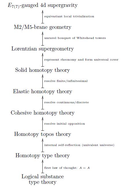
Including in homotopy type theory the progression of modal operators that we have found above
makes its term model richer: there are now true propositions and generally terms that may be constructed which are not constructible in plain homotopy type theory. These terms reflect the idea that is induced by these determinations, in that every interpretation of this modal type theory has to realize (externalize) these terms and make these propositions true.
We now indicate some of these new constructions.
Maurer-Cartan forms
Let be a an ∞-group type. This means that there is specified a pointed connected type and an equivalence with its loop space object. We say that is the delooping of . Notice that all this happens internal to the ambient cohesive homotopy type theory, which makes have the interpretation of the moduli ∞-stack of cohesive -principal ∞-bundles, instead of just the bare homotopy type of the classifying space
This richer geometric structure is what the boldface in is meant to remind us of.
Definition
Denote the first and second homotopy fiber of the comparison map of the flat moment of this as follows.
This double homotopy fiber has the interpretation of being the Maurer-Cartan form on .
Differential cohomology
Let be an abelian ∞-group type. The group of phases.
This being abelian just means that there is specified a delooping type and an equivalence with its loop space object, and that with we have inductively that is itself equipped with the structure of an abelian ∞-group.
For the present purpose we will assume in addition that is 0-truncated, which makes it simply an abelian group.
Definition
A Hodge filtration is a compatible system of filtrations of of the form
with 0-truncated extensive .
Definition
Given a Hodge filtration, write for the homotopy fiber product
of the Maurer-Cartan form with the last Holdge filtration stage.
Proposition
The decomposition of into its -moments according to prop reproduces the defining Cartesian sqare of def. :
WZW terms
A map
is equivalently a cocycle of degree in the group cohomology of .
Definition
Given a group cocycle and a Hodge filtration, then a refinement of the Hodge filtration along the group cocycle is a chose of 0-trucated extensive fitting into a square
Given this, write
Example
For 0-truncated, then the canonical choice is . With this one has .
On the other extreme, for then the canonical choice is . With this one has .
This means that in general is a homotopy fiber product of with , hence that a map to out of some is a pair of a map and of -form data on . This is the kind of field content of higher gauged WZW models.
Proposition
Given a group cocycle and a form refinement as in def. , then there exists an essentially unique prequantization
of whose underlying -principal ∞-bundle is .
-Manifolds
See also at geometry of physics – manifolds and orbifolds.
Definition
Given then a morphism is a local diffeomorphism if its naturality square of the infinitesimal shape modality
is a pullback square.
Remark
The abstract definition comes down to being the appropriate synthetic differential supergeometry-version of the traditional statement that is a local diffeomorphism if the diagram of tangent bundles
To see this, notice by the discussion at synthetic differential geometry that for an infinitesimally thickened point, then for any the mapping space is the jet bundle of with jets of order as encoded by the infinitesimal order of . In particular if is the first order infinitesimal interval defined by the fact that its algebra of functions is the algebra of dual numbers , and is a smooth manifold, then
is the ordinary tangent bundle of . Now use that the internal hom preserves limits in its second argument, and that, by the hom-adjunction, and finally use that .
Let now be given, equipped with the structure of a group (infinity-group).
Definition
A -manifold is an such that there exists a -atlas, namely a correspondence of the form
with both morphisms being local diffeomorphisms, def. , and the right one in addition being an epimorphism, hence an atlas.
Proposition
If is a local diffeomorphism, def. , then so is image under the bosonic modality.
Proof
Since the bosonic modality provides Aufhebung for we have . Moreover anyway. Finally preserves pullbacks (being in particular a right adjoint). Hence hitting a pullback diagram
with yields a pullback diagram
Frame bundles
Definition
Given , its infinitesimal disk bundle is the pullback of the unit of the infinitesimal shape modality along itself
Given a point , then the infinitesimal neighbourhood of that point is the further pullback of the infinitesimal disk bundle to this point:
More generally, for then the th order infinitesimal disk bundle is
and accordingly the th order infinitsimal neighbourhood is
It is natural not to pick any point, but to collect all infinitesimal disks around all the points of a space:
Definition
The relative flat modality is the operation that sends to the homotopy pullback
More generally, for any then the order relative flat modality is the pullback in
Definition
The general linear group is the automorphism infinity-group of the infinitesimal neighbourhood , def. , of the neutral element :
Proposition
For a -manifold, def. , then its infinitesimal disk bundle , def. , is associated to a -principal – to be called the frame bundle, modulated by a map to be called , producing homotopy pullbacks of the form
Definition
A framing of a -manifold is a trivialization of its frame bundle, prop. , hence a diagram in of the form
Remark
It is useful to express def. in terms of the slice topos . Write for the canonical morphism regarded as an object in the slice. Then a framing as in def. is equivalently a morphism
in .
Proposition
The group object , canonically regarded as a -manifold, carries a canonical framing, def. , , induced by left translation.
-Structure
See also at geometry of physics – G-structure and Cartan geometry.
Definition
Given a homomorphism of groups , a G-structure on a -manifold is a lift of the frame bundle of prop. through this map
Remark
As in remark , it is useful to express def. in terms of the slice topos . Write for the given map regarded as an object in the slice. Then a -structure according to def. is equivalently a choice of morphism in of the form
In other words, is the moduli stack for -structures.
Example
A choice of framing , def. , on a -manifold induces a G-structure for any , given by the pasting diagram in
or equivalently, via remark and remark , given as the composition
We call this the left invariant -structure.
Definition
For a -manifold, then a G-structure on , def. , is integrable if for any -atlas the pullback of the -structure on to is equivalent there to the left-inavariant -structure on of example , i.e. if we have an correspondence in the double slice topos of the form
The -structure is infintesimally integrable if this holds true after restriction along the relative shape modality , def. , to all the infinitesimal disks in :
Finally, the -structure is order infinitesimally integrable if this holds for the order- relative shape modality .
Definition
Consider an infinity-action of on which linearizes to the canonical -action on by def. . Form the semidirect product . Consider any group homomorphism .
A -Cartan geometry is a -manifold equipped with a -structure, def. . The Cartan geometry is called (infinitesimally) integrable if the -structure is so, according to def. .
Remark
For an abelian group, then in traditional contexts the infinitesimal integrability of def. comes down to the torsion of a G-structure vanishing. But for a nonabelian group, this definition instead enforces that the torsion is on each infinitesimal disk the intrinsic left-invariant torsion of itself.
Traditionally this is rarely considered, matching the fact that ordinary vector spaces, regarded as translation groups , are abelian groups. But super vector spaces regarded (in suitable dimension) as super translation groups are nonabelian groups. Therefore super-vector spaces may carry intrinsic torsion, and therefore first-order integrable -structures on -manifolds are torsion-ful.
Indeed, this is a phenomenon known as the torsion constraints in supergravity. Curiously, as discussed there, for the case of 11-dimensional supergravity the equations of motion of the gravity theory are equivalent to the super-Cartan geometry satisfying this torsion constraint. This way super-Cartan geometry gives a direct general abstract route right into the heart of M-theory.
Definite forms
Definition
Given a group cocycle with WZW term, prop. , of the form
and given a -manifold we say that an integrable globalization of over is a WZW on on
such that there is a -atlas for
which extends to a correspondence between and
Accordingly, as in def. we say that is an infinitesimally integrable globalization if this correspondence exists after restriction along the inclusion of the infinitesimal disks in and such that
-
the induced section of the associated -fiber infinity-bundle is definite on the restriction of to the infinitesimal disk;
-
also the underlying cocycle is definite, in that the infinitesimal disk bundle lifts to an -gerbe (for the induced group structure on ).
If had no higher gauge transformations, then this would already ensure that such a globalization globalizes locally cohesively, but here in higher differential geometry this property becomes genuine structure and hence we need to demand it. There is an axiomatic way to say this (see dcct for details) and if this is imposed then we say that is a definite globalization of .
Proposition
There is a canonical (∞,1)-functor from (infinitesimally integrable) definite globalizations of over a -manifold to (infinitesimally integrable) -structures on , def. , for
the intensification (in the sense above) of the stabilizer ∞-group of the restriction of along the inclusion of the typical infinitesimal disk .
Nature
Given a theory of physics, made sufficiently precise in formal logic, then an interpretation of the theory by a model “is” nature as predicted by this theory.
For instance if we considered Einstein gravity to be the theory of pseudo-Riemannian manifolds subject to some energy condition, then a model for this theory is one concrete particular spacetime.
Above we saw that cohesive (elastic) homotopy type theory contains Cartan geometry, hence in particular pseudo-Riemannian geometry in its idea, as well as gauge theory and hence we accordingly find models of nature here.
Recall specifically that
-
From prop. we have that group cocycles of degree induce WZW terms in that degree and hence the WZW sigma model prequantum field theory on the worldvolume of a p-brane propagating on the “model spacetime” .
-
A second cocycle on the infinity-group extension classified by yields a type of -brane on which these -branes may end;
-
This structure is naturally generalized to -manifolds equipped with definite globalizations of these WZW terms, defining -branes propagating on .
-
The definite globalization of the WZW term induces a structure on and the requirement that this be infinitesimally integrable is a torsion constraint on .
We now find an externalization of the idea such that
-
There is a canonical bouquet of higher group cocycles and their ∞-group extensions emanating from the unique 0-truncated purely fermionic type – the superpoint.
-
The resulting branes and their intersection laws are those seen in string theory;
-
The resulting spacetimes are superspacetimes as in the relevant supergravity theories;
-
The resulting torsion constraints, namely the supergravity torsion constraints, imply, in the maximally extended situation, the Einstein equations of motion of 11-dimensional supergravity, specifically of d=4 N=1 supergravity arising in the guise of M-theory on G2-manifolds.
This is a “theory of everything” in the sense of modern fundamental physics, which is beeing argued to have viable phenomenology, see at G2-MSSM for more on this. Even if it turns out that there are no models in this theory which match quantitative measurements in experiment, it is noteworthy that the qualitative structure of this theory is that of Einstein-Yang-Mills-Dirac-Higgs theory and hence matches faithfully the qualitative features of nature that is in experiment. Given our starting point above this is maybe not to be lightly dismissed.
Externalization
Theorem
The cohesive+elastic+solid homotopy type theory above has a faithful (i.e. non-degenerate) categorical semantics in the homotopy topos of super formal smooth infinity-groupoids.
We now spell out the construction of this model and indicate the proof of this statement.
Definition
Write
-
CartSp for the site of Cartesian spaces;
-
for the category of first-order infinitesimally thickened points (i.e. the formal duals of commutative algebras over the real numbers of the form with a finite-dimensional square-0 nilpotent ideal).
-
for the category of superpoints, by which we here mean the formal duals to commutative superalgebras which are super-Weil algebras.
There are then “semidirect product” sites and (whose objects are Cartesian products of the given form inside synthetic differential supergeometry and whose morphisms are all morphisms in that context (not just the product morphisms)).
Set then
for the collection of smooth ∞-groupoids;
for the collection of formal smooth ∞-groupoids (see there) and finally
for that of super formal smooth ∞-groupoids.
Proposition
The sites in question are alternatingly (co-)reflective subcategories of each other (we always display left adjoints above their right adjoints)
Here
-
the first inclusion picks the terminal object ;
-
the second inclusion is that of reduced objects; the coreflection is reduction, sending an algebra to its reduced algebra;
-
the third inclusion is that of even-graded algebras, the reflection sends a -graded algebra to its even-graded part, the co-reflection sends a -graded algebra to its quotient by the ideal generated by its odd part, see at superalgebra – Adjoints to the inclusion of plain algebras.
Passing to (∞,1)-categories of (∞,1)-sheaves, this yields, via (∞,1)-Kan extension, a sequence of adjoint quadruples as follows:
the total composite labeled is indeed the locally constant infinity-stack-functor.
Forming adjoint triples from these adjoint quadruples gives idempotent (co-)monads
satisfying the required inclusions of their images.
Proof
All the sites are ∞-cohesive sites, which gives that we have an cohesive (infinity,1)-topos. The composite inclusion on the right is an ∞-cohesive neighbourhood site, whence the inclusion exhibits differential cohesion.
With this the rightmost adjoint quadruple gives the Aufhebung of by and the further opposition .
Remark
The model in def. admits also the refinement of the infinitesimal shape modality to an infinite tower
characterizing th order infinitesimals. Let
be the stratification of by its full subcategories on those objects whose coresponding Weil algebras/local Artin algebras are of the form with . Each of these inclusions has coreflection, given by projection onto the quotient by the ideal , as ranges
Proof
The first two items follow with the discussion at ∞-cohesive site. The second two by dcct, prop. 5.2.51.
Proof
For the statement consider the following:
Since the site of has a terminal object , it follows that for any sheaf then
(where we may leave the constant re-embedding implicit, due to it being fully faithful).
Moreover, for every object there exists a morphism hence for every and every there exists a morphism . This means that if then for all and hence .
We now show that this condition is equivalent to the required Aufhebung:
Generally, given a topos equipped with a level of a topos given by an adjoint modality , then the condition is equivalent to .
Because: in a topos the initial object is a strict initial object, and hence . Therefore in one direction, assuming then
Conversely, assuming that , then for all
and hence by the Yoneda lemma .
Second, for the statement consider the following:
For any and any we have by adjunction natural equivalences
Here the crucial step is the observation that on representables, by construction, the reduced part of the even part is the reduced part of the original object.
But observe that
Proof
The definition would require that
is an epimorphism. But this is equivalent to the point inclusion
into the formal dual of the algebra of dual numbers.
Space-Time-Matter
We discuss now how in the externalization of the theory given by theorem there naturally appears spacetime from the idea.
The progressive system of moments above, yields, by prop. , two god-given objects:
| real line | superpoint |
|---|---|
Both have familiar structure of an abelian group object, being the additive group, hence there are arbitrary deloopings and .
Given two types, there are the judgements in which these appear as subject and as predicate, in the sense discussed above.
There are no non-trivial judgements with (a delooping of) as the subject and (a delooping of) as the predicate. But there turn out to be some exceptional judgements with subject and predicate .
By example this leads to the deduction of the object which is the homotopy fibers of the corresponding maps. From these one obtains further judgements, then further objects, and so forth. This way a “bouquet” of objects is induced from the initial ones.
We now discuss how this bouquet first of all yields super Minkowski spacetime (Huerta-Schreiber 17) and then further the extended super Minkowski spacetimes arising from super p-brane condensates (FSS).
Minkowski spacetime
Consider first the superpoint .
Remark
This is the unique 0-truncated object which is
-
purely negative to bosonic moment;
-
purely opposite to bosonic moment;
in that
Since (and the other objects obtained in a moment) are contractible as super Lie groups, we may use the van Est isomorphism to conveniently discuss them as super Lie algebras. Regarding as a super Lie algebra, then its Chevalley-Eilenberg algebra is freely generated from a -bigraded element
It is evident that
Proposition
The second super Lie algebra cohomology of is
represented by the 2-cocycles of the form
classified by this is the super translation group in 1-dimension.
This is the worldline of the superparticle.
There are no further non-trivial cocycles here giving further extensions.
Hence next consider the Cartesian product of the initial superpoint with itself.
Remark
This is still purely of negative bosonic moment in that , but it no longer has purely no moment opposed to bosonic moment (witnessing that the fermionic opposition is not complete, lemma ), instead
is the first-order infinitesimal interval (the formal dual of the “algebra of dual numbers”).
Proposition
The second super Lie algebra cohomology of is
represented by the cocycles of the form
The extension classified by this
is 3-dimensional super Minkowski spacetime.
Proof
This follows by inspection of the real spin representations in dimension 3, see the details spelled out at spin representation – via division algebras – Example d=3).
For more on this see at geometry of physics – supersymmetry the section Supersymmetry from the Superpoint.
Now the old brane scan gives:
Proposition
The -invariant third Lie algebra cohomology of 3d Minkowski super-spacetime is
represented by the 3-cocycle which, as a left invariant super differential form on is the WZW term in the Green-Schwarz action functional for the super 1-brane in 3d.
A definite globalization, of this 3-cocycle over a -manifold requires, by def. , that the tangent bundle is a bundle of super Lie algebras and that the cocycle extends to a definite form. This imposes G-structure for the Lorentz group (or rather its spin group double cover).
Proposition
The joint stabilizer of of the Lie bracket and the 3-cocycle is the pin group , the unoriented generalization of the spin group , the double cover of the Lorentz group .
This is one special case of a more general statement which we come to as prop. below.
Consider then
Proposition
There is a 1-dimensional space of -invariant 2-cocycles on . The Lie algebra extension classified by that is 4d super Minkowski spacetime
Proof
By inspection of the real spin representations in dimension 4.
Now the old brane scan gives:
Proposition
represented by the 4-cocycle which, as a left invariant super differential form on is the WZW term in the Green-Schwarz action functional for the super 2-brane in 4d.
Lorentz symmetry
Notice that so far we have obtained 3-dimensional and 4-dimensional Minkowski spacetime and the WZW-term for the superstring and the membrane propagating on it without assuming knowledge of the Lorentz group. In fact we assumed nothing but the presence of the real line and the odd line and we have simply investigated their cohomology.
The following proposition shows that the Lorentz group, in fact its universal cover by the pseudo-Riemannian spin group is deduced from this.
Proposition
Let be super Minkowski spacetime in dimension and let the corresponding 3-form characterizing the super-1-brane (superstring) in this dimension, according to the brane scan . Then the stabilizer subgroup of both the super Lie bracket and the cocycle is the Spin group :
Proof
It is clear that the spin group fixes the cocycle, and by the discussion at spin representation it preserves the bracket. Therefore it remains to be seen that the Spin group already exhausts the stabiizer group of bracket and cocycle. For that observe that the 3-cocycle is
where is the given Minkowski metric, and that the bilinear map
is surjective. This imples that if preserves both the bracket and the cocycle for all and to
then it preserves the Minkowski metric for all
This means that -manifolds equipped with the 3-cocycle as a definite form such that the resulting G-structure according to prop. also preserves the the group structure on , then this is equivalent to equipping with Lorentzian orthogonal structure, hence with super-pseudo-Riemannian metric, hence with a field-configuration for 3d supergravity.
Fundamental branes
The brane bouquet that we find…
this is equivalently the physics coming from M-theory on G2-manifolds, given by the extensions that emanate from 32 copies of the smallest superpoint:
These are branches of The brane bouquet of string theory, see there for more. By prop. each branch here gives the WZW form for the corresponing Green-Schwarz super p-brane sigma model.
Gravity
Above we have found two interlocking ingredients arising from the axiomatics:
-
abstract generals – Given any group object , then there is an abstract general concept of -manifolds , def. . Given furthermore a WZW term on , then there is an abstract general concept of definite globalizations of this term over these manifolds , inducing G-structures on , prop. .
-
concrete individuals – We have found concrete individual s: extended super Minkowski spacetimes, prop. , prop. emanating from the objects which represent the moments and , and we have further found individual : the super p-brane WZW terms, prop. etc., forming The brane bouquet.
Plugging the concrete individuals into the general abstract theory, we hence obtain particular phenomena.
Specifically there is 11-dimensional super Minkowski spacetime carrying the WZW term for the M2-brane, in some sense the endpoint of the bouquet of super-spacetimes. The KK-compactification of this on a 7-dimensional G2-manifold yields the 4-dimensional super-Minkowski spacetime discussed above, with the WZW term for the super 2-brane in 4d.
The 11-dimensional super-Minkowski spacetime is special in many ways, one of which is that in this dimension the equations of motion of 11-dimensional supergravity on a -super Cartan geometry modeled on are already captured by just a constraint on the torsion tensor. But by remark this means that in dimension 11 the equations of motion of supergravity have an immediate axiomatization in our objective logic.
equivalent to just the condition that the of is at each point and to first infinitesimal order the intrinsic torsion of
Proposition
First-order integrable -super-Cartan geometries, def. , on -manifolds , def. , which are first-order integrable with respect to the intrinsic left-invariant torsion of , remark , are equivalent to vacuum solutions to the equations of motion of 11-dimensional supergravity, i.e. to solutions for which the field strength of the gravitino and of the supergravity C-field vanishes identically, hence to solutions to the ordinary vacuum Einstein equations in 11d.
Proof
(Howe 97) shows that imposing (on some chart) implies (and hence is equivalent to) the equations of motion of 11d supergravity. These equations (see e.g. D’Auria-Fré 82, p. 31) then show that furthermore requiring (and hence requiring the full supertorsion tensor to be that of super-Minkowski spacetime) puts the field strength of the gravitino and of the supergravity C-field to 0.
Remark
Vacuum Einstein solutions as in prop. , are considered notably in the context of M-theory on G2-manifolds (e.g. Acharya 02, p. 9). See also at M-theory on G2-manifolds – Details – Vacuum solution and torsion constraints.
Proposition
Given a definite globalization of a super -brane WZW term , then the stabilizer infinity-group of is the integrated BPS charge algebra of this solution of supergravity.
See at BPS charge – Formalization in higher differential geometry.
Acknowledgements
These notes benefited from discussion with Dave Carchedi, David Corfield, Thomas Holder, John Huerta and Mike Shulman.
References
-
Ulrich Bunke, Thomas Nikolaus, Michael Völkl, Differential cohomology theories as sheaves of spectra, Journal of Homotopy and Related Structures, October 2014 (arXiv:1311.3188)
-
Domenico Fiorenza, Hisham Sati, Urs Schreiber, Super Lie n-algebra extensions, higher WZW models and super p-branes with tensor multiplet fields, Volume 12, Issue 02 (2015) 1550018
-
John Huerta, Urs Schreiber, M-Theory from the Superpoint (arXiv:1702.01774)
-
Peter Johnstone, Sketches of an Elephant – A Topos Theory Compendium, Oxford 2002.
-
James Ladyman, Stuart Presnell, Does Homotopy Type Theory Provide a Foundation for Mathematics?, 2014 (web)
-
William Lawvere, Some Thoughts on the Future of Category Theory in A. Carboni, M. Pedicchio, G. Rosolini, Category Theory , Proceedings of the International Conference held in Como, Lecture Notes in Mathematics 1488, Springer (1991)
-
William Lawvere, Toposes of laws of motion, Sept. 1997 (pdf)
-
William Lawvere, Axiomatic cohesion Theory and Applications of Categories, Vol. 19, No. 3, 2007, pp. 41-49. (web, pdf)
-
Dan Licata, Mike Shulman, Adjoint logic with a 2-category of modes, Logical Foundations of Computer Science, Volume 9537 of the series Lecture Notes in Computer Science pp 219-235, 2015 (pdf)
-
Per Martin-Löf, An intuitionistic theory of types: predicative part, In Logic Colloquium (1973), ed. H. E. Rose and J. C. Shepherdson (North-Holland, 1974), 73-118. (web)
-
Thomas Nikolaus, Urs Schreiber, Danny Stevenson, Principal ∞-Bundles – General theory, Journal of Homotopy and Related Structures, June 2014 (arXiv:1207.0248)
-
Arhtur Sale, Primitive data types, The Australian Computer Journal, Vol. 9, No. 2, July 1977 (pdf)
-
Michael Shulman, Univalence for inverse diagrams and homotopy canonicity, Mathematical Structures in Computer Science, Volume 25, Issue 5 ( From type theory and homotopy theory to Univalent Foundations of Mathematics ) June 2015 (arXiv:1203.3253, doi:/10.1017/S0960129514000565)
-
Michael Shulman, Inductive and higher inductive types (2012) (pdf)
-
Michael Shulman, model of type theory in an (infinity,1)-topos
-
Mike Shulman, Brouwer’s fixed-point theorem in real-cohesive homotopy type theory, Mathematical Structures in Computer Science Vol 28 (6) (2018): 856-941 (arXiv:1509.07584, doi:10.1017/S0960129517000147)
-
Univalent Foundations Project, Homotopy Type Theory – Univalent Foundations of Mathematics, 2013
Related talks include
Last revised on May 23, 2025 at 17:26:26. See the history of this page for a list of all contributions to it.