nLab basic complex line bundle on the 2-sphere

Idea

The basic line bundle on the 2-sphere is the complex line bundle on the 2-sphere whose first Chern class is a generator $\pm 1 \in \mathbb{Z} \,\simeq\, H^2(S^2, \mathbb{Z})$, equivalently the tautological line bundle on the Riemann sphere regarded as complex projective 1-space.

This is the pullback bundle of the map $S^2 \to B U(1) \simeq B^2 \mathbb{Z}$ to the classifying space/Eilenberg-MacLane space which itself represents a generator of the homotopy group $\pi_2(S^2) \simeq \mathbb{Z}$.

Beware that this basic line bundle is sometimes called the “canonical line bundle on the 2-sphere”, but it is not isomorphic to what in complex geometry is called the canonical bundle of the 2-sphere regarded as a Riemann surface. Instead it is “one half” of the latter, its theta characteristic. See also at geometric quantization of the 2-sphere.

The basic line bundle is the canonically associated bundle to basic principal U(1)-bundle: the complex Hopf fibration. Another name for it is the tautological line bundle for the complex projective line $\mathbb{P}^1(\mathbb{C})$ (the Riemann sphere), namely the map $\mathbb{C}^2 \setminus \{(0, 0)\} \to \mathbb{P}^1(\mathbb{C})$ mapping $(x, y)$ to $[x; y]$.

Definition

The classifying space for principal U(1)-bundles, or equivalently (via forming associated bundles) that of complex line bundles is $B U(1)$, which as a Grassmannian is the infinite complex projective space $\mathbb{C}P^\infty$. The homotopy type of this space is that of the Eilenberg-MacLane space $K(\mathbb{Z},2)$. This means that $K(\mathbb{Z},2)$ is in particular path-connected and has second homotopy group the integers: $\pi_2(K(\mathbb{Z},2)) \simeq \mathbb{Z}$.

It being the classifying space for complex line bundles means that

$$\left\{ \array{ \text{isomorphism classes of} \\ \text{complex line bundles} \\ \text{on}\,\, S^2 } \right\} \;\simeq\; \left\{ \array{ \text{continuous functions} \\ S^2 \longrightarrow K(\mathbb{Z},2) \\ \text{up to homotopy} } \right\} \;\simeq\; \pi_2(K(\mathbb{Z},2)) \;\simeq\; \mathbb{Z} \,.$$

The (isomorphism class) of the complex line bundle which corresponds to $+1 \in \mathbb{Z}$ under this sequence of isomorphisms is called the basic complex line bundle on the 2-sphere.

Hence the basic complex line bundle on the 2-sphere is the pullback bundle of the universal complex line bundle on $B U(1)$ along the map $S^2 \to B U(1)$ which represents the element $1 \in \mathbb{Z} \simeq \pi_2(B U(1))$. If the classifying space $B U(1)$ is represented by the infinite complex projective space $\mathbb{C}P^\infty$ with its canonical CW-complex structure (this prop.), then this map is represented by the canonical cell inclusion $S^2 \hookrightarrow\mathbb{C}P^\infty$.

Notice that there is a non-trivial automorphism of $\mathbb{Z}$ as an abelian group given by $n \mapsto -n$. This means that there is an ambiguity in the definition of the basic line bundle on the 2-sphere.

Properties

General

Lemma

(clutching construction of the basic line bundle)

Under the clutching construction of vector bundles on the 2-sphere, the basic complex line bundle on the 2-sphere is given by the transition function

$$\mathbb{C} \supset \, S^1 \longrightarrow GL(1,\mathbb{C}) \, \subset \mathbb{C}$$

from the Euclidean circle $S^1 \subset \mathbb{R}^2 \simeq \mathbb{C}$ to the complex general linear group in 1-dimension, which is $GL(1,\mathbb{C}) \simeq \mathbb{C} \setminus \{0\}$ given simply by

$$z \mapsto z \,,$$

Alternatively, due to the sign ambiguity in the definition of the basic bundle, its clutching transition function is given by

$$z \mapsto - z \,.$$

Proof

Under the clutching construction the isomorphism class of a complex line bundle corresponds to the homotopy class of its clutching transition function

$$S^1 \to GL(1, \mathbb{C}) \simeq \mathbb{C} \setminus \{0\}$$

hence to an element of the fundamental group $\pi_1(\mathbb{C} \setminus \{0\}) \simeq \mathbb{Z}$. Hence by definition, the basic bundle has clutching transition function corresponding to $\pm 1 \in \mathbb{Z} \simeq [S^1, GL(1,\mathbb{Z})]$ and this element is represented by the function $z \mapsto \pm z$.

Proposition

(fundamental tensor/sum relation of the basic complex line bundle)

Under direct sum of vector bundles $\oplus_{S^2}$ and tensor product of vector bundles $\otimes_{S^2}$, the basic line bundle on the 2-sphere $H \to S^2$ satisfies the following relation

$$H \oplus_{S^2} H \;\simeq\; \left( H \otimes_{S^2} H \right) \oplus_{S^2} 1_{S^2}$$

(where $1_{S^2}$ denotes the trivial vector bundle complex line bundle on the 2-sphere).

(e.g (Hatcher, Example 1.13))

Proof

Via the clutching construction there is a single transition function of the form

$$S^1 \longrightarrow GL(n,\mathbb{C})$$

that characterizes all the bundles involved. With $S^1 \hookrightarrow \mathbb{C}$ identified with the topological subspace of complex numbers of unit absolute value, the standard choice for these functions is

• for the trivial line bundle $1_{S^2}$ we may choose

  $f_1 \colon z \mapsto \left( 1 \right)$;

• for the basic line bundle we may choose (by lemma )

  $f_H \colon z \mapsto \left( z\right)$

This yields

• for $H \otimes H \oplus 1_{S^2}$ the clutching function

  $z \mapsto \left( \array{ z^2 & 0 \\ 0 & 1 }\right)$

• for $H \oplus H$ the clutching function

  $z \mapsto \left( \array{ z & 0 \\ 0 & z } \right)$.

Since the complex general linear group $Gl(n,\mathbb{C})$ is path-connected (by this prop.), there exists a continuous function

$$\gamma \colon [0,1] \longrightarrow GL(2,\mathbb{C})$$

connecting the identity matrix on $\mathbb{C}^2$ with the one that swaps the two entries, i.e.

with $\gamma(0) = \left( \array{ 1 & 0 \\ 0 & 1 } \right)$

and $\gamma(1) = \left( \array{ 0 & 1 \\ 1 & 0 } \right)$

Therefore the function

$$\array{ S^1 \times [0,1] &\overset{}{\longrightarrow}& GL(2,\mathbb{C}) \\ (z,t) &\overset{\phantom{AA}}{\longrightarrow}& f_{H \oplus 1}(z) \cdot \gamma(t) \cdot f_{1 \oplus H}(z) \cdot \gamma(t) }$$

(with matrix multiplication on the right) is a left homotopy from $f_{H \oplus H}$ to $f_{H \otimes H \oplus 1}$.

Remark

(fundamental product theorem in topological K-theory)

Under the map

$$Vect(S^2)_{/\sim} \longrightarrow K(X)$$

that sends complex vector bundles to their class in the topological K-theory ring $K(X)$, the fundamental tensor/sum relation of prop. says that the K-theory class $H$ of the basic line bundle in $K(X)$ satisfies the relation

$$\begin{aligned} (H - 1)^2 & = H^2 + 1 - \underset{= H^2 + 1}{\underbrace{2 H}} \\ = & 0 \end{aligned}$$

in $K(X)$.

(Notice that $H-1$ is the image of $[H]$ in the reduced K-theory $\tilde K(X)$ of $S^2$ under the splitting $K(X) \simeq \tilde K(X) \oplus \mathbb{Z}$ (by this prop.).)

It follows that there is a ring homomorphism of the form

$$\array{ \mathbb{Z}[h]/\left( (h-1)^2 \right) &\overset{}{\longrightarrow}& K(S^2) \\ h &\overset{\phantom{AAA}}{\mapsto}& H }$$

from the polynomial ring in one abstract generator, quotiented by this relation, to the topological K-theory ring.

It turns out that this homomorphism is in fact an isomorphism, hence that the relation $(H-1)^2 = 0$ from prop. is the only relation satisfied by the basic complex line bundle in topological K-theory.

More generally, for $X$ a topological space, then there is a composite ring homomorphism

$$\array{ K(X) \otimes \mathbb{Z}[h]/((h-1)^2) & \longrightarrow & K(X) \times K(S^2) & \longrightarrow & K(X \times S^2) \\ (E, h) &\overset{\phantom{AAA} }{\mapsto}& (E,H) &\overset{\phantom{AAA}}{\mapsto}& (\pi_{X}^\ast E) \cdot (\pi_{S^2}^\ast H) }$$

to the topological K-theory ring of the product topological space $X \times S^2$, where the second map is the external tensor product of vector bundles.

This composite is an isomorphism if $X$ is a compact Hausdorff space (for $X = \ast$ the point space this reduces to the previous statement).

This is called the fundamental product theorem in topological K-theory. It is the main ingredient in the proof of Bott periodicity in complex topological K-theory.

As an index bundle

We discuss how the basic complex line bundle on $S^2$ is isomorphically the subbundle of +1 eigenspaces of a natural $S^2$-parameterized Dirac-like linear operator acting on $\mathbb{C}^2$, which gives its natural realization as a Fredholm index bundle (cf. Rem. below). This kind of construction plays a key role in the discussion of Chern insulators (topological phases of matter with nontivial first Chern class of the valence bundle, cf. Rem. below).

To this end, consider:

• $\mathbb{H}$ the real star-algebra of quaternions, with norm given by ${\vert q \vert}^2 \coloneqq q q^\ast$,

• $\mathbb{H}_{im} \subset \mathbb{H}$ the subspace of imaginary quaternions ($q \in \mathbb{H}$ such that $q^\ast = - q$), in which we choose, as usual, an orthonormal linear basis $\mathbf{i}, \mathbf{j}, \mathbf{k}$ such that $\mathbf{i} \mathbf{j} = \mathbf{k}$,

• $\mathbb{H} \longrightarrow End(\mathbb{C}^2)$ the star-algebra homomorphism which identifies the unit imaginary quaternions with Pauli matrices:

  $$\begin{array}{rcr} \mathbb{H} &\overset {\phantom{--} \sigma \phantom{--}} {\longrightarrow}& End(\mathbb{C}^2) \\ 1 &\mapsto& \left[\begin{matrix} \phantom{+}1 & \phantom{+}0 \\ \phantom{+}0 & \phantom{+}1 \end{matrix}\right] \\ \mathbf{i}\, &\mapsto& \mathrm{i} \left[\begin{matrix} \phantom{+}1 & \phantom{+}0 \\ \phantom{+}0 & -1 \end{matrix}\right] \\ \mathbf{j}\, &\mapsto& \mathrm{i} \left[\begin{matrix} \phantom{+}0 & \phantom{+}1 \\ \phantom{+}1 & \phantom{+}0 \end{matrix}\right] \\ \mathbf{k}\, &\mapsto& \mathrm{i} \left[\begin{matrix} \phantom{+}0 & \phantom{+}\mathrm{i} \\ -\mathrm{i} & \phantom{+}0 \end{matrix}\right] \mathrlap{\,,} \end{array}$$

• $S(\mathbb{H})$ the 3-sphere of unit norm quaternions, which by the above homomorphism is identified with the special unitary matrices,

  $$S(\mathbb{H}) \underoverset {\sim} {\phantom{--} \sigma \phantom{--}} {\longrightarrow} SU(2)$$

  because

  $$\begin{array}{l} det\big( x_0 \mathrm{id} + x_1 \sigma_{\mathbf{i}} + x_2 \sigma_{\mathbf{j}} + x_3 \sigma_{\mathbf{k}} \big) \\ \;=\; det \left[ \begin{matrix} x_0 + \mathrm{i} x_1 & \mathrm{i}x_2 - x_3 \\ \mathrm{i} x_2 + x_3 & x_0 - \mathrm{i} x_1 \end{matrix} \right] \\ \;=\; (x_0)^2 + (x_1)^2 + (x_2)^2 + (x_3)^2 \end{array}$$

  and

  $$\begin{array}{l} \big( x_0 \mathrm{id} + x_1 \sigma_{\mathbf{i}} + x_2 \sigma_{\mathbf{j}} + x_3 \sigma_{\mathbf{k}} \big)^\dagger \big( x_0 \mathrm{id} + x_1 \sigma_{\mathbf{i}} + x_2 \sigma_{\mathbf{j}} + x_3 \sigma_{\mathbf{k}} \big) \\ \;=\; \big( x_0 \mathrm{id} - x_1 \sigma_{\mathbf{i}} - x_2 \sigma_{\mathbf{j}} - x_3 \sigma_{\mathbf{k}} \big) \big( x_0 \mathrm{id} + x_1 \sigma_{\mathbf{i}} + x_2 \sigma_{\mathbf{j}} + x_3 \sigma_{\mathbf{k}} \big) \\ \;=\; (x_0)^2 + (x_1)^2 + (x_2)^2 + (x_3)^2 \,, \end{array}$$

• the group action of $SU(2) \simeq Spin(3)$ through SO(3) on $\mathbb{H}_{im} \simeq_{{}_{\mathbb{R}}} \mathbb{R}^3$ given by

  $$\begin{array}{ccc} \overset{ Spin(3) \times \mathbb{R}^3 }{ \overbrace{ S(\mathbb{H}) \times \mathbb{H}_{im} } } &\longrightarrow& \overset{ \mathbb{R}^3 }{ \overbrace{ \mathbb{H}_{im} } } \\ (q, x) &\mapsto& q x q^\ast \mathrlap{\,,} \end{array}$$

• $S(\mathbb{H}_{im})$ the 2-sphere of unit-norm imaginary quaternions.

Observing that the complex Hopf fibration is equivalently (see there):

$$\begin{array}{c} S(\mathbb{H}) &\overset {\phantom{--} h_{\mathbb{C} \phantom{--}} } {\longrightarrow} & S(\mathbb{H}_{im}) \\ q &\mapsto& q \cdot \mathbf{i} \cdot q^\ast \end{array}$$

whose fiber over $\mathbf{i}$ is

$$\begin{array}{rcl} \overset{ \mathrm{U}(1) }{ \overbrace{ S(\mathbb{C}) } } &\xhookrightarrow{\phantom{---}}& \overset{ \mathrm{SU}(2) }{ \overbrace{ S(\mathbb{H}) } } \\ x + y \mathrm{i} &\mapsto& x + y \mathbf{i} \,, \end{array}$$

it follows that the basic complex line bundle on the 2-sphere is the associated complex line bundle

$$S^3 \times_{\mathrm{U}(1)} \mathbb{C} \;=\; \Big\{ (q,z) \in S(\mathbb{H}) \times \mathbb{C} \Big\}_{ \big/\big( (q,z) \sim (q \alpha^\ast, \alpha z) \;\forall_{\alpha \in S(\mathbb{C})}\, \big) } \,.$$

As such, this is a subbundle of the trivial complex vector bundle of rank$=2$, via this map: This subbundle is evidently characterized as the bundle of +1 eigenspaces of this $S^2$-parameterized linear operator:

(1)$$\begin{array}{rrcl} S(\mathbb{H}) &\overset{\phantom{--} - \mathrm{i}\, \sigma \phantom{--}}{\longrightarrow}& End(\mathbb{C}^2) \\ q \mathbf{i} q^\ast &\mapsto& -\mathrm{i} \sigma_{ q \mathbf{i} q^\ast } \end{array} \;\;\;\; \text{hence equivalently of} \;\;\;\; \begin{array}{rrcl} S^2 &\overset{\phantom{--} H \phantom{--}}{\longrightarrow}& End(\mathbb{C}^2) \\ \vec x \equiv (x^1, x^2, x^3) &\mapsto& -\mathrm{i} \big( x^1 \sigma_{\mathbf{i}} + x^2 \sigma_{\mathbf{j}} + x^3 \sigma_{\mathbf{k}} \big) \,. \end{array}$$

(This statement, without proof, may be found for instance in Baum 2015 slide 32, Baum & Erp 2018 p 106-107).

Remark

(relation to Chern insulators) The normalized Hamiltonians (1) play a key role in solid state physics in the discussion of 2D 2-band crystals such as notably considered as models for Chern insulators (like the Haldane model, cf. Sticlet et al 2012 (2-3)).

It follows from the above discussion that

1. any continuous family of such operators over a Brillouin torus $T^2$ is given by a continuous map $f \colon T^2 \longrightarrow{} S^2$,

2. the +1 eigenspace bundle of the corresponding family of operators on $T^2$ (the valence bundle in these models) has first Chern class equal to the pullback along $f$ of the generating class $1 \in H^2(S^2;\mathbb{Z})$ of the basic line bundle on $S^2$.

Similar arguments are ubiquituous in the literature on Chern insulators (cf. Sticlet et al 2012 p 2), though the concrete statement that all these constructions amount to pulling back the Bott generator along a map to the 2-sphere may not have been made explicit elsewhere.

Remark

(As a Fredholm index bundle)
With the basic line bundle realized as the kernel bundle of a $\mathbb{C}P^1$-parameterized projection operator $P_{(-)} \colon \mathbb{C}^2 \to \mathbb{C}^2$, there is a a nice way to produce also a $\mathbb{C}P^1$-parameterized Fredholm operator

(2)$$\begin{array}{rcl} S^2 &\overset{F_{(-)}}{\longrightarrow}& Fred(\mathscr{H}) \mathrlap{\,,} \end{array}$$

whose index bundle represents the class of the basic line bundle in topological K-theory under the Atiyah-Jänich theorem, like this:

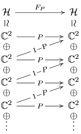
This is a Fredholm operator with $ker(F_P) = ker(P)$ and $coker(F_P) = 0$.

Remark

The first presentation in (1) makes manifest that the map $S^2 \longrightarrow End(\mathbb{C}^2)$ is $Spin(3)$-equivariant: with respect to the rotation action through $SO(3)$ on the left and the conjugation action by special unitary matrices in $SU(2) \simeq Spin(3)$ on the right.

From this it follows that also the corresponding parameterized Fredholm operator (2) is $Spin(3)$-equivariant, if we let $Spin(3) \simeq SU(2)$ act on

$$\mathscr{H} \,\simeq\, \mathbb{C}^2 \oplus \ell_2(\mathbb{N}) \,\simeq\, \bigoplus_{\mathbb{N}} \mathbb{C}^2$$

as the infinite direct sum of the defining representation of $SU(2)$.

The resulting $Spin(3)$-equivariant family of Fredholm operators should the the representation of the tautological equivariant line bundle in the equivariant K-theory of $S^2$.

Related concepts

• universal complex line bundle

• tautological line bundle, equivariant tautological line bundle

References

• Allen Hatcher: Vector bundles and K-Theory, book draft (2017) [webpage, pdf]

• Klaus Wirthmüller, Vector bundles and K-theory (2012) [pdf]

• Paul Baum, slide 32 of: Dirac operator, lecture at TIFR Mumbai, India (2015) [pdf, pdf]

• Paul Baum, Erik van Erp, 2.11 of: $K$-homology and Fredholm operators I: Dirac operators, Journal of Geometry and Physics 134 (2018) 101-118 [doi:10.1016/j.geomphys.2018.08.008]