nLab embedding of differentiable manifolds

Idea

Embeddings of differentiable manifolds are submanifold inclusions.

Definition

Classical definition

Definition

(embedding of smooth manifolds)

An embedding of smooth manifolds is a smooth function $f : X \hookrightarrow Y$ between smooth manifolds $X$ and $Y$ such that

1. $f$ is an immersion;

2. the underlying continuous function is an embedding of topological spaces.

A closed embedding is an embedding such that the image $f(X) \subset Y$ is a closed subset.

Synthetic definition in differential cohesion

The classical definition of embedding of smooth manifolds should have the following axiomatization in differentially cohesive infinity-topos theory, where one assumes the following system of adjoint modalities

$$\array{ && \Re &\dashv& \Im &\dashv& \& \\ && && \vee && \vee \\ && && ʃ &\dashv& \flat &\dashv& \sharp }$$

Of these we now use

1. the sharp modality $\sharp$

2. the infinitesimal shape modality $\Im$.

Then given a morphism $U \overset{i}{\longrightarrow} X$ we have

1. $i$ being a monomorphism means that it is a monomorphism in an (infinity,1)-category

2. $i$ being an immersion means (by this Discussion) that it is a formally unramified morphism in that the comparison morphism

   $$U \longrightarrow X \times_{\Im X} \Im(U)$$

   into the pullback along the $\Im$-unit is a monomorphism;

3. $i$ being an embedding means (by this Discussion) that the comparison morphism

   $$U \longrightarrow X \times_{\sharp X} \sharp U$$

   is an equivalence.

In terms of cohesive homotopy type theory this should mean that the characteristic function

$$\chi_U \;\colon\; X \longrightarrow Type$$

to the type universe, of $U$ regarded as a dependent type over $X$, satisfies:

1. it factors through the universe of propositions $Prop$, hence of $\vert -\vert_{-1}$-modal types (where $\vert-\vert_{-1}$ is the (-1)-truncation modality);

2. it factors through the universe of $\Im$-submodal types?;

3. it factors through the universe of $\sharp$-modal types.

Examples

Nonexample

(immersions that are not embeddings)

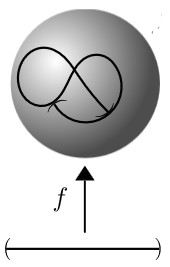
Consider an immersion $f \;\colon\; (a,b) \to \mathbb{R}^2$ of an open interval into the Euclidean plane (or the 2-sphere) as shown on the right. This is not a embedding of smooth manifolds: around the points where the image crosses itself, the function is not even injective, but even a#t the points where it just touches itself, the pre-images under $f$ of open subsets of $\mathbb{R}^2$ do not exhaust the open subsets of $(a,b)$, hence do not yield the subspace topology.

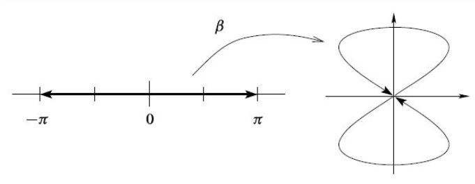
As a concrete examples, consider the function $(sin(2-), sin(-)) \;\colon\; (-\pi, \pi) \longrightarrow \mathbb{R}^2$. While this is an immersion and injective, it fails to be an embedding due to the points at $t = \pm \pi$ “touching” the point at $t = 0$.

graphics grabbed from Lee

Properties

Basic properties

Proposition

(proper injective immersions are equivalently the closed embeddings)

Let $X$ and $Y$ be smooth manifolds, and let $f \colon X \to Y$ be a smooth function. Then the following are equivalent

1. $f$ is a proper injective immersion;

2. $f$ is a closed embedding (def. ).

Proof

Since topological manifolds are locally compact topological spaces (this example), this follows directly since injective proper maps into locally compact spaces are equivalently closed embeddings.

Proposition

(submanifolds admit slice charts) For $X$ a smooth manifold and $\iota \colon \Sigma \hookrightarrow X$ the embedding of a submanifold, then there exists slice charts:

For each point $\sigma \in \Sigma$ there is a coordinate chart $X \supset U \xrightarrow{\phi} \mathbb{R}^n$ of $X$ such that $\sigma \in U \subset M$ and $\phi(\Sigma \cap U)$ is a rectilinear hyperplane in $\phi(U) \subset \mathbb{R}^n$.

(e.g. Lee 2012, Thm. 5.8)

hupf

Embedding into Euclidean space

Every smooth manifold has a embedding of smooth manifolds into a Euclidean space $\mathbb{R}^k$ of some dimension $k$.

For compact smooth manifolds this is easy to see (prop. below), while the generalization to non-compact smooth manifolds requires a tad more work (theorem below). What is non-trivial is to find the minimum dimension of the ambient Euclidean space for which embedding in general still exist. The Whitney embedding theorem (prop. below) says that this is twice the dimension of the manifolds to be embedded.

Proposition

For every compact smooth manifold $X$ (of finite dimension), there exists some $k \in \mathbb{N}$ such that $X$ has an embedding (def. ) into the Euclidean space of dimension $k$:

$$X \overset{\text{embd}}{\hookrightarrow} \mathbb{R}^k$$

Proof

Let

$$\{\mathbb{R}^n \underoverset{\simeq}{\phi_i}{\longrightarrow} U_i \subset X\}_{i \in I}$$

be an atlas exhibiting the smooth structure of $X$. In particular this is an open cover, and hence by compactness there exists a finite subset $J \subset I$ such that

$$\{\mathbb{R}^n \underoverset{\simeq}{\phi_i}{\to} U_i \subset X\}_{i \in J \subset I}$$

is still an open cover.

Since $X$ is a smooth manifold, there exists a partition of unity $\{f_i \in C^\infty(X,\mathbb{R})\}_{i \in J }$ subordinate to this cover with smooth functions $f_i$ (by this prop.).

This we may use to extend the inverse chart identifications

$$X \supset \;\; U_i \underoverset{\simeq}{\psi_i}{\longrightarrow} \mathbb{R}^n$$

to smooth functions

$$\hat \psi_i \;\colon\; X \to \mathbb{R}^{n}$$

by setting

$$\hat \psi_i \;\colon\; x \mapsto \left\{ \array{ f_i(x) \cdot \psi_i(x) &\vert& x \in U_i \subset X \\ 0 &\vert& \text{otherwise} } \right. \,.$$

The idea now is to combine all these functions to obtain an injective function

$$(\hat \psi_i)_{i \in J} \;\colon\; X \longrightarrow (\mathbb{R}^n)^{\vert J\vert } \simeq \mathbb{R}^{n \cdot {\vert J \vert }} \,.$$

But while this is injective, it need not be an immersion, since the derivatives of the product functions $f_i \cdot \psi_i$ may vanish, even though the derivatives of the two factors do not vanish separately. However this is readily fixed by adding yet more ambient coordinates and considering the function

$$(\hat \psi_i, f_i)_{i \in I} \;\colon\; X \longrightarrow \left(\mathbb{R}^{n+1}\right)^{\vert J \vert} \simeq \mathbb{R}^{(n+1)\cdot {\vert J \vert}} \,.$$

This is an immersion. Hence it remains to see that it is also an embedding of topological spaces.

By this prop it is sufficient to see that the injective continuous function is a closed map. But this follows generally since $X$ is a compact topological space by assumption, and since Euclidean space is a Hausdorff topological space, and since maps from compact spaces to Hausdorff spaces are closed and proper.

Proposition

For every smooth manifold $X$ of dimension $n$ (Hausdorff, sigma-compact), there exists some $k \in \mathbb{N}$ such that $X$ has an embedding into the Euclidean space of dimension $k$.

What is harder to prove is that $k$ may be chosen to be as small as $2n$

Proposition

(Whitney's strong embedding theorem)

For every smooth manifold $X$ of dimension $n$ (Hausdorff, sigma-compact), there is an embedding into the Euclidean space of dimension $2n$.

In fact this bound is minimal, there are smooth manifolds of dimension $n$ which have no embdding into $\mathbb{R}^k$ for $k \lt 2n$.

Space of Embeddings

This section follows from a discussion on the Algebraic Topology mailing list as to making concrete the contractibility of the space of embeddings of a smooth manifold in $\mathbb{R} ^{(\infty )}$, the union of the Euclidean spaces. There are two parts to showing that this space is contractible. The first is showing that it is not empty. The second is to exhibit a contraction.

Showing that it is not empty is a partition of unity argument. As the space that we are embedding in is infinite dimensional, we do not need to resort to either compactness or Whitney’s embedding theorem to obtain an embedding. One of these would be required if we wanted to show that our embedding was actually in some finite Euclidean space.

The contraction depends on certain properties of $\mathbb{R} ^{(\infty )}$ which are quite general and seemingly unrelated to the question of embeddings. The key property is the existence of a shift map. The same idea is used in showing that many other related spaces are contractible, including the infinite sphere.

Existence of Embeddings

Theorem

Let $M$ be a smooth manifold. Let $V$ be an infinite dimensional locally convex topological vector space. Then there is an embedding (def. ) $M \hookrightarrow V$.

Proof

We shall start with the case $V = \mathbb{R} ^{(\infty )}$. The more general case will follow from that.

As $M$ is a smooth manifold, we can choose a partition of unity $\{ \rho _{i} : i \in I\}$ on $M$ with the property that for each $\rho _{i}$, its support is contained in the domain of some chart for $M$ and the family of those domains is locally finite. Let us suppose that these charts are $\phi _{i} \colon U_{i} \to \mathbb{R} ^{n}$, where $n = \dim M$. As $M$ is second countable, this partition of unity will be countable.

Using the partition of unity, we extend $\phi _{i} \colon U_{i} \to \mathbb{R} ^{n}$ to a smooth map $\psi _{i} \colon M \to \mathbb{R} ^{n+1}$ by setting, for $x \in U_{i}$, $\psi _{i}(x) = (\rho _{i}(x) \phi _{i}(x),\rho _{i}(x))$ and, for $x \notin U_{i}$, $\psi _{i}(x) = 0$. Using the $\psi _{i}$ we define $\psi \colon M \to \mathbb{R} ^{(\infty )}$ by $\psi (x) = (\psi _{i}(x))$. This is well-defined as, for any $x \in M$, there are only finitely many of the $\rho _{i}$ for which $\rho _{i}(x) \ne 0$ and thus only finitely many of the $\psi _{i}$ for which $\psi _{i}(x) \ne 0$. We define $\psi \colon M \to V$ by composing this with the inclusion $\mathbb{R} ^{(\infty )} \to V$.

We claim that this is an embedding.

The first thing to show is that it is continuous. Let $x \in M$. Then there is some $i$ such that $x \in U_{i}$. As the family $U_{i}$ is locally finite, there are only a finite number of other $U_{j}$ with non-trivial intersection with $U_{i}$. Thus there are only a finite number of $\rho _{j}$ which take non-zero values on $U_{i}$. Hence the image of $U_{i}$ under $\psi$ lies in some $\mathbb{R} ^{k}$ and the induced map $U_{i} \to \mathbb{R} ^{k}$ is built up from a finite number of the $\phi _{j}$ and $\rho _{j}$, whence is continuous. Hence $\psi$ is continuous.

The next thing to show is that it is injective. Suppose that $x,y \in M$ are such that $\psi (x) = \psi (y)$. As the partition of unity functions can be recovered from $\psi$, we must therefore have $\rho _{i}(x) = \rho _{i}(y)$ for all $i$. Since $\{ \rho _{i}\}$ is a partition of unity, there must be some $i$ such that $\rho _{i}(x) \ne 0$ (whence also $\rho _{i}(y) \ne 0$). This means that $x$ and $y$ lie in the domain of the chart $\phi _{i}$. Moreover, as $\psi (x) = \psi (y)$, we must have $\psi _{i}(x) = \psi _{i}(y)$. Lastly, as $\rho _{i}(x) = \rho _{i}(y)$ and this is non-zero, we have $\phi _{i}(x) = \phi _{i}(y)$. Therefore $x = y$.

We want to show that $\psi$ is a topological embedding. To do this, we consider first what happens to the sets $\rho _{i}^{-1}(0,\infty )$. Pick some $i \in I$. Let $p_{i} \colon \mathbb{R} ^{(\infty )} \to \mathbb{R} ^{n+1}$ be the projection onto the $n + 1$ coordinates corresponding to the position of $\psi _{i}$ in $\psi$, so that $p_{i} \psi = \psi _{i}$. Let $W \subseteq \mathbb{R} ^{n+1}$ be the open subset where the last coordinate is non-zero. Then $p_{i}^{-1}(W)$ is open in $\mathbb{R} ^{(\infty )}$. Now $x \in \psi (M) \cap p_{i}^{-1}(W)$ if and only if $\rho _{i}(x) \ne 0$, thus:

$$\psi (M) \cap p_{i}^{-1}(W) = \psi (\rho _{i}^{-1}(0,\infty )).$$

We define a map $W \to \mathbb{R} ^{n}$ by $(x,t) \mapsto t^{-1} x$. The composition

$$\rho _{i}^{-1}(0,\infty ) \xrightarrow{\psi } p_{i}^{-1}(W) \xrightarrow{p_{i}} W \to \mathbb{R} ^{n}$$

is then seen to be the same as the restriction of $\phi _{i}$ to $\rho _{i}^{-1}(0,\infty )$. As $\phi _{i}$ is a homeomorphism and $\rho _{i}$ is continuous, the above map $\rho _{i}^{-1}(0,\infty ) \to \mathbb{R} ^{n}$ is a homeomorphism onto its image which is an open subset of $\mathbb{R} ^{n}$.

We therefore see that if $V \subseteq \rho _{i}^{-1}(0,\infty )$ is open then $\psi (V)$ is equal to the inverse image of $\phi _{i}(V)$ under the composition $p_{i}^{-1}(W) \to W \to \mathbb{R} ^{n}$ and is thus open in $\psi (M)$.

Now suppose that $V \subseteq M$ is an arbitrary open subset. Then for each $i \in I$, $V \cap \rho _{i}^{-1}(0,\infty )$ is open and the union of these is $V$. So $\psi (V)$ is the union of $\psi (V \cap \rho _{i}^{-1}(0,\infty ))$ and thus is open in $\psi (M)$. Hence $\psi$ is an embedding.

To complete the proof for $\mathbb{R} ^{(\infty )}$, we need to show that $\psi$ is an immersion. This is a local condition and follows from the fact that we can recover $\phi _{i}$ from $\psi _{i}$.

The case for an arbitrary $V$ is a simple adaptation of the above. As $V$ is infinite dimensional, it admits linear injections $\mathbb{R} ^{(\infty )} \to V$ and composing one of those with $\psi$ gives an injective map $M \to V$. To ensure that it is an embedding, we need suitable projections $V \to \mathbb{R} ^{n+1}$. To know that these exist, we simply choose our map $\mathbb{R} ^{(\infty )} \to V$ carefully as follows. Pick a non-zero vector $v_{1} \in V$. By the Hahn-Banach theorem, there is some $f_{1} \in V^{*}$ with $f_{1}(v_{1}) = 1$. Now choose a non-zero $v_{2} \in \ker f_{1}$. Again, we have $f_{2} \in V^{*}$ such that $f_{2}(v_{2}) = 1$ and $f_{2}(v_{1}) = 0$. By construction, $f_{1}(v_{1}) = 0$ also. We continue this recursively, choosing at each stage a non-zero $v_{k} \in \bigcap \ker f_{j}$ and $f_{k} \in V^{*}$ with $f_{k}(v_{k}) = 1$ and $f_{k}(v_{j}) = 0$ for $j \lt k$. The result is an injection $\mathbb{R} ^{(\infty )} \to V$ together with functions $f_{j} \in V^{*}$ such that the composition $\mathbb{R} ^{(\infty )} \to V \xrightarrow{f_{j}} \mathbb{R}$ is the $j$th coordinate function.

With an assumption on $V$ and a careful choice of partition of unity, we can ensure that our embedding so constructed has closed image.

Theorem

Let $M$ be a smooth manifold. Let $V$ be a locally convex topological vector space and assume that there exists a family of continuous linear functionals $\{f_j : j \in \mathbb{N}\} \subseteq V^*$ with the properties:

1. For $j \in \mathbb{N}$, $f_j$ is non-trivial on $\bigcap_{k \ne j} \ker f_k$, and
2. The family of functionals $\{\sum_{j \in F} f_j : {|F|} \lt \infty\}$ is equicontinuous

then there is an embedding $\psi \colon M \to V$ with closed image.

Proof

From the first property, we can find $v_j \in \bigcap_{k \ne j} \ker f_k$ such that $f_j(v_j) = 1$. We use the family $\{v_j\}$ to define a linear injection $\mathbb{R}^{(\infty)} \to V$ (continuous by necessity). The functionals $f_j$ provide the necessary coordinate projections so that the proof of Theorem works.

In addition, we shall assume that our partition of unity used in the proof of Theorem is such that the functions therein have compact support.

Let $(x_\lambda)$ be a net in $M$ for which $(\psi(x_\lambda))$ converges in $V$, say to $x$. The assumption on the functionals is there to show that $x \ne 0$. Let us show why this is the case. For a finite set $F \subseteq \mathbb{N}$, let $f_F = \sum_{j \in F} f_j$. The assumption of equicontinuity means that $\bigcap_F f_F^{-1}(-1,1)$ is an open neighbourhood of $0$ in $V$. Now for each $y \in M$, there is some finite $F \subseteq \N$ for which $\sum f_j(y) = 1$. This is because we can choose $F$ to correspond to those terms in the partition of unity which are non-zero on $y$. Hence $\psi(M)$ has empty intersection with the above neighbourhood of $0$, and so no net in $\psi(M)$ can converge to $0$.

Thus $x \ne 0$ and, moreover, there is some finite $F \subseteq \mathbb{N}$ for which $f_F(x) \ne 0$ and thus there is some $j \in \mathbb{N}$ for which $f_j(x) \ne 0$. Since $(\psi(x_\lambda)) \to x$, there is therefore a cofinal subset on which $f_j$ is never zero. Let us pass to that subnet. Now on $M$, the functions $f_i \circ \psi$ are either the functions in the partition of unity or are dominated by them. Hence there is some $i \in \mathbb{N}$ with the property that for all $\lambda$, $\rho_i(x_\lambda) \ne 0$ (now that we’ve passed to the subnet). This means that $(x_\lambda)$ lies in the support of $\rho_i$, which is (by the first assumption) a compact subset of $M$. It therefore has a convergent subnet with limit, say $x'$. But by continuity of $\psi$ and uniqueness of limits in $V$, it must be the case that $\psi(x') = x$.

Hence $\psi(M)$ is closed in $V$.

There are various situations in which it is straightforward to find a suitable family of functionals. If $V$ is barrelled, then finding a family for which $\sum f_j$ weakly converges will do since then the family of partial sums is simply bounded and hence, as $V$ is barrelled, equicontinuous.

Thus the coordinate projections will do for $\mathbb{R}^{(\infty)}$ and for $\ell^1$. For $\ell^2$ we can take weighted projections, say $f_j = \frac{1}{j} p_j$. In this case, our dual vectors will be $\{j e_j\}$. For $\ell^\infty$ we can take weighted projections corresponding to a sequence in $\ell^1$.

It is interesting to note what is going on in these latter cases where we take weighted projections. If we embedded our manifold using the standard basis vectors as our “anchor points” then the structure of the ambient space is insufficient to guarantee that our manifold does not contain a convergent net with limit point outside. More exactly, there could be a net in our manifold such that in the image it converges to zero. The partition of unity is not enough to keep our points away from zero, since as we get further along the family in our partition we could need more and more terms. That is, we could have the situation where we have a sequence $(x_n)$ in $M$ where $x_n$ is “seen” by $n$ of the functions in the partition of unity. Then we could have $\psi(x_n)$ to be something like $(0,\dots,0,1/n,1/n,\dots,1/n,0,\dots)$. In, say, $\ell^2$ then this sequence converges to $0$. Essentially, $\psi(x_n)$ gets more and more diffuse. Introducing the weights, or rather their inverses, counters this by ensuring that terms “far down” the sequence are given more consideration.

Contractibility of Embeddings

Once we know that the space of embeddings of a compact smooth manifold in $\mathbb{R} ^{(\infty )}$ is not empty, its contractibility follows from rather general properties. It follows from the existence of a split map.

Theorem

Let $M$ be a smooth manifold. Let $V$ be a locally convex topological vector space which admits a split map. Then the space of embeddings, $\Emb(M,V)$, is contractible.

Proof

Recall that to have a split map on $V$ means that we have a decomposition $V \cong V \oplus V$ with a non-degeneracy property. This implies that one of the induced maps $V \to V$, called the splitting map, has no eigenvectors.

Let $S^{+} \colon V \to V$ be a splitting map and let $S^{-}$ be the remainder. Then the map $H \colon [0,1] \colon V \to V$ given by $H(t,v) = H_{t}(v) = (1 - t) v + t S^{+} v$ is a homotopy between the identity on $V$ and $S^{+}$.

At $t = 0$, $H_{t} = I$ which is an inclusion. For $t \ne 0$ then if $H_{t}(v) = 0$ we have that $S^{+} v = t^{-1}(1 - t) v$ whence $v$ is an eigenvector of $S^{+}$. But the assumption that $S^{+}$ is a splitting map includes the property that it has no eigenvectors, and thus $H_{t}$ is an inclusion for all $t$. Moreover, $H_{t}$ is an embedding for all $t$ since $I = H_{t} + t S^{-} v$.

Hence we can apply $H_{t}$ to $\Emb(M,V)$ to obtain a homotopy between the identity on $\Emb(M,V)$ and the inclusion of $\Emb(M,V)$ in itself as the subspace of all embeddings that lie in the even subspace.

Now we pick some embedding $\psi _{0} \colon M \to V$ which, by applying $S^{-}$ if necessary, we assume to exist in the image of $S^{-}$. We define a homotopy $G_{t}$ on the embedding space by $G_{t}(\psi ) = t \psi _{0} + (1 - t) \psi$, using the additive structure in $V$. That this passes through the space of embeddings is clear since for $t \ne 1$ we can recover the embedding $\psi _{0}$ by composing with $S^{-}$. Combining $H_{t}$ and $G_{t}$ as homotopies leads to the desired contraction of the embedding space.

Related concepts

• submanifold

• Whitney embedding theorem, Nash embedding theorem

• hypersurface

References

Monographs:

• William M. Boothby, Def. III 4.11 in: An introduction to differentiable manifolds and Riemannian geometry, Academic Press (1975, 1986), Elsevier (2002) [ISBN:9780121160517, pdf]

• John Lee, Chapter 5 of: Introduction to Smooth Manifolds, Springer (2012) [doi:10.1007/978-1-4419-9982-5, book webpage, pdf]

Lecture notes:

• Paul Rapoport, Introduction to Immersion, Embedding and the Whitney Embedding Theorem, 2015 (pdf)

• Emery Thomas, Embedding manifolds in Euclidean space, Osaka Journal Mathematics 13 (1976) (pdf)

• Rodolfo De Sapio, Embedding $\pi$-manifolds, Annals of mathematics, Second Series, Vol 82, No 2 (jstor)

• Manifold Atlas, Embeddings in Euclidean space: an introduction to their classification

Discussion of embeddings of spheres into each other (generalizing the concept of knots):

• André Haefliger, Differentiable Embeddings of $S^n$ in $S^{n+q}$ for $q \gt 2$, Annals of Mathematics Second Series, Vol. 83, No. 3 (May, 1966), pp. 402-436 (jstor:1970475)

• Dennis Roseman, Masamichi Takase, High-codimensional knots spun about manifolds (arXiv:math/0609055)

References

Original articles:
- André Haefliger: Plongements différentiables de variétés dans variétés, Commentarii mathematici Helvetici 36 (1961/62) 47-82 [eudml:139228, pdf]