nLab Introduction to Cobordism and Complex Oriented Cohomology

---

$\,$

This page collects introductory seminar notes to the concepts of generalized (Eilenberg-Steenrod) cohomology theory, basics of cobordism theory and complex oriented cohomology.

$\,$

The category of those generalized cohomology theories that are equipped with a universal “complex orientation” happens to unify within it the abstract structure theory of stable homotopy theory with the concrete richness of the differential topology of cobordism theory and of the arithmetic geometry of formal group laws, such as elliptic curves. In the seminar we work through classical results in algebraic topology, organized such as to give in the end a first glimpse of the modern picture of chromatic homotopy theory.

$\,$

For background on stable homotopy theory see Introduction to Stable homotopy theory.

For application to/of the Adams spectral sequence see Introduction to the Adams Spectral Sequence

$\,$

---

$\,$

$\,$

Outline. We start with two classical topics of algebraic topology that first run independently in parallel:

• 1) Generalized cohomology

• 2) Cobordism theory

The development of either of these happens to give rise to the concept of spectra and via this concept it turns out that both topics are intimately related. The unification of both is our third topic

• 3) Complex oriented cohomology

$\,$

Literature. (Kochman 96).

Generalized cohomology

Idea. The concept that makes algebraic topology be about methods of homological algebra applied to topology is that of generalized homology and generalized cohomology: these are covariant functors or contravariant functors, respectively,

$$Spaces \longrightarrow Ab^{\mathbb{Z}}$$

from (sufficiently nice) topological spaces to $\mathbb{Z}$-graded abelian groups, such that a few key properties of the homotopy types of topological spaces is preserved as one passes them from Ho(Top) to the much more tractable abelian category Ab.

Literature. (Aguilar-Gitler-Prieto 02, chapters 7,8 and 12, Kochman 96, 3.4, 4.2, Schwede 12, II.6)

Generalized cohomology functors

Idea. A generalized (Eilenberg-Steenrod) cohomology theory is such a contravariant functor which satisfies the key properties exhibited by ordinary cohomology (as computed for instance by singular cohomology), notably homotopy invariance and excision, except that its value on the point is not required to be concentrated in degree 0. Dually for generalized homology. There are two versions of the axioms, one for reduced cohomology, and they are equivalent if properly set up.

An important example of a generalised cohomology theory other than ordinary cohomology is topological K-theory. The other two examples of key relevance below are cobordism cohomology and stable cohomotopy.

Literature. (Switzer 75, section 7, Aguilar-Gitler-Prieto 02, section 12 and section 9, Kochman 96, 3.4).

$\,$

Reduced cohomology

The traditional formulation of reduced generalized cohomology in terms of point-set topology is this:

Definition

A reduced cohomology theory is

1. a functor

   $$\tilde E^\bullet \;\colon\; (Top^{\ast/}_{CW})^{op} \longrightarrow Ab^{\mathbb{Z}}$$

   from the opposite of pointed topological spaces (CW-complexes) to $\mathbb{Z}$-graded abelian groups (“cohomology groups”), in components

   $$\tilde E \;\colon\; (X \stackrel{f}{\longrightarrow} Y) \mapsto (\tilde E^\bullet(Y) \stackrel{f^\ast}{\longrightarrow} \tilde E^\bullet(X)) \,,$$

2. equipped with a natural isomorphism of degree +1, to be called the suspension isomorphism, of the form

   $$\sigma_E \;\colon\; \tilde E^\bullet(-) \overset{\simeq}{\longrightarrow} \tilde E^{\bullet +1}(\Sigma -)$$

such that:

1. (homotopy invariance) If $f_1,f_2 \colon X \longrightarrow Y$ are two morphisms of pointed topological spaces such that there is a (base point preserving) homotopy $f_1 \simeq f_2$ between them, then the induced homomorphisms of abelian groups are equal

   $$f_1^\ast = f_2^\ast \,.$$

2. (exactness) For $i \colon A \hookrightarrow X$ an inclusion of pointed topological spaces, with $j \colon X \longrightarrow Cone(i)$ the induced mapping cone (def.), then this gives an exact sequence of graded abelian groups

   $$\tilde E^\bullet(Cone(i)) \overset{j^\ast}{\longrightarrow} \tilde E^\bullet(X) \overset{i^\ast}{\longrightarrow} \tilde E^\bullet(A) \,.$$

(e.g. AGP 02, def. 12.1.4)

This is equivalent (prop. below) to the following more succinct homotopy-theoretic definition:

Definition

A reduced generalized cohomology theory is a functor

$$\tilde E^\bullet \;\colon\; Ho(Top^{\ast/})^{op} \longrightarrow Ab^{\mathbb{Z}}$$

from the opposite of the pointed classical homotopy category (def., def.), to $\mathbb{Z}$-graded abelian groups, and equipped with natural isomorphisms, to be called the suspension isomorphism of the form

$$\sigma \;\colon\; \tilde E^{\bullet +1}(\Sigma -) \overset{\simeq}{\longrightarrow} \tilde E^\bullet(-)$$

such that:

• (exactness) it takes homotopy cofiber sequences in $Ho(Top^{\ast/})$ (def.) to exact sequences.

As a consequence (prop. below), we find yet another equivalent definition:

Definition

A reduced generalized cohomology theory is a functor

$$\tilde E^\bullet \;\colon\; (Top^{\ast/})^{op} \longrightarrow Ab^{\mathbb{Z}}$$

from the opposite of the category of pointed topological spaces to $\mathbb{Z}$-graded abelian groups, such that

• (WHE) it takes weak homotopy equivalences to isomorphisms

and equipped with natural isomorphism, to be called the suspension isomorphism of the form

$$\sigma \;\colon\; \tilde E^{\bullet +1}(\Sigma -) \overset{\simeq}{\longrightarrow} \tilde E^\bullet(-)$$

such that

• (exactness) it takes homotopy cofiber sequences in $Ho(Top^{\ast/})$ (def.), to exact sequences.

Proposition

The three definitions

• def.

• def.

• def.

are indeed equivalent.

Proof

Regarding the equivalence of def. with def. :

By the existence of the classical model structure on topological spaces (thm.), the characterization of its homotopy category (cor.) and the existence of CW-approximations, the homotopy invariance axiom in def. is equivalent to the functor passing to the classical pointed homotopy category. In view of this and since on CW-complexes the standard topological mapping cone construction is a model for the homotopy cofiber (prop.), this gives the equivalence of the two versions of the exactness axiom.

Regarding the equivalence of def. with def. :

This is the universal property of the classical homotopy category (thm.) which identifies it with the localization (def.) of $Top^{\ast/}$ at the weak homotopy equivalences (thm.), together with the existence of CW approximations (rmk.): jointly this says that, up to natural isomorphism, there is a bijection between functors $F$ and $\tilde F$ in the following diagram (which is filled by a natural isomorphism itself):

$$\array{ Top^{op} &\overset{F}{\longrightarrow}& Ab^{\mathbb{Z}} \\ {}^{\mathllap{\gamma_{Top}}}\downarrow & \nearrow_{\mathrlap{\tilde F}} \\ Ho(Top)^{op}\simeq (Top_{CW})/_\sim }$$

where $F$ sends weak homotopy equivalences to isomorphisms and where $(-)_\sim$ means identifying homotopic maps.

Prop. naturally suggests (e.g. Lurie 10, section 1.4) that the concept of generalized cohomology be formulated in the generality of any abstract homotopy theory (model category), not necessarily that of (pointed) topological spaces:

Definition

Let $\mathcal{C}$ be a model category (def.) with $\mathcal{C}^{\ast/}$ its pointed model category (prop.).

A reduced additive generalized cohomology theory on $\mathcal{C}$ is

1. a functor

   $$\tilde E^\bullet \;\colon \; Ho(\mathcal{C}^{\ast/})^{op} \longrightarrow Ab^{\mathbb{Z}}$$

2. a natural isomorphism (“suspension isomorphisms”) of degree +1

   $$\sigma \; \colon \; \tilde E^\bullet \longrightarrow \tilde E^{\bullet+1} \circ \Sigma$$

such that

• (exactness) $\tilde E^\bullet$ takes homotopy cofiber sequences to exact sequences.

Finally we need the following terminology:

Definition

Let $\tilde E^\bullet$ be a reduced cohomology theory according to either of def. , def. , def. or def. .

We say $\tilde E^\bullet$ is additive if in addition

• (wedge axiom) For $\{X_i\}_{i \in I}$ any set of pointed CW-complexes, then the canonical morphism

  $$\tilde E^\bullet(\vee_{i \in I} X_i) \longrightarrow \prod_{i \in I} \tilde E^\bullet(X_i)$$

  from the functor applied to their wedge sum (def.), to the product of its values on the wedge summands, is an isomorphism.

We say $\tilde E^\bullet$ is ordinary if its value on the 0-sphere $S^0$ is concentrated in degree 0:

• (Dimension) $\tilde E^{\bullet\neq 0}(\mathbb{S}^0) \simeq 0$.

If $\tilde E^\bullet$ is not ordinary, one also says that it is generalized or extraordinary.

A homomorphism of reduced cohomology theories

$$\eta \;\colon\; \tilde E^\bullet \longrightarrow \tilde F^\bullet$$

is a natural transformation between the underlying functors which is compatible with the suspension isomorphisms in that all the following squares commute

$$\array{ \tilde E^\bullet(X) &\overset{\eta_X}{\longrightarrow}& \tilde F^\bullet(X) \\ {}^{\mathllap{\sigma_E}}\downarrow && \downarrow^{\mathrlap{\sigma_F}} \\ \tilde E^{\bullet + 1}(\Sigma X) &\overset{\eta_{\Sigma X}}{\longrightarrow}& \tilde F^{\bullet + 1}(\Sigma X) } \,.$$

We now discuss some constructions and consequences implied by the concept of reduced cohomology theories:

Definition

Given a generalized cohomology theory $(E^\bullet,\delta)$ on some $\mathcal{C}$ as in def. , and given a homotopy cofiber sequence in $\mathcal{C}$ (prop.),

$$X \stackrel{f}{\longrightarrow} Y \stackrel{g}{\longrightarrow} Z \stackrel{coker(g)}{\longrightarrow} \Sigma X \,,$$

then the corresponding connecting homomorphism is the composite

$$\partial \;\colon\; \widetilde E^\bullet(X) \stackrel{\sigma}{\longrightarrow} \widetilde E^{\bullet+1}(\Sigma X) \stackrel{coker(g)^\ast}{\longrightarrow} \widetilde E^{\bullet+1}(Z) \,.$$

Proposition

The connecting homomorphisms of def. are parts of long exact sequences (the long exact sequences in generalized cohomology):

$$\cdots \stackrel{\partial}{\longrightarrow} \widetilde E^{\bullet}(Z) \longrightarrow \widetilde E^\bullet(Y) \longrightarrow \widetilde E^\bullet(X) \stackrel{\partial}{\longrightarrow} \widetilde E^{\bullet+1}(Z) \to \cdots \,.$$

Proof

By the defining exactness of $\widetilde E^\bullet$, def. , and the way this appears in def. , using that $\sigma$ is by definition an isomorphism.

Unreduced cohomology

Given a reduced generalized cohomology theory as in def. , we may “un-reduce” it and evaluate it on unpointed topological spaces $X$ simply by evaluating it on $X_+$ (def.). It is conventional to further generalize to relative cohomology and evaluate on unpointed subspace inclusions $i \colon A \hookrightarrow X$, taken as placeholders for their mapping cones $Cone(i_+)$ (prop.).

In the following a pair $(X,U)$ refers to a subspace inclusion of topological spaces $U \hookrightarrow X$. Whenever only one space is mentioned, the subspace is assumed to be the empty set $(X, \emptyset)$. Write $Top_{CW}^{\hookrightarrow}$ for the category of such pairs (the full subcategory of the arrow category of $Top_{CW}$ on the inclusions). We identify $Top_{CW} \hookrightarrow Top_{CW}^{\hookrightarrow}$ by $X \mapsto (X,\emptyset)$.

Definition

A cohomology theory (unreduced, relative) is

1. a functor

   $$E^\bullet : (Top_{CW}^{\hookrightarrow})^{op} \to Ab^{\mathbb{Z}}$$

   to the category of $\mathbb{Z}$-graded abelian groups,

2. a natural transformation of degree +1, to be called the connecting homomorphism, of the form

   $$\delta_{(X,A)} \;\colon\; E^\bullet(A, \emptyset) \to E^{\bullet + 1}(X, A) \,.$$

such that:

1. (homotopy invariance) For $f \colon (X_1,A_1) \to (X_2,A_2)$ a homotopy equivalence of pairs, then

   $$E^\bullet(f) \;\colon\; E^\bullet(X_2,A_2) \stackrel{\simeq}{\longrightarrow} E^\bullet(X_1,A_1)$$

   is an isomorphism;

2. (exactness) For $A \hookrightarrow X$ the induced sequence

   $$\cdots \to E^n(X, A) \longrightarrow E^n(X) \longrightarrow E^n(A) \stackrel{\delta}{\longrightarrow} E^{n+1}(X, A) \to \cdots$$

   is a long exact sequence of abelian groups.

3. (excision) For $U \hookrightarrow A \hookrightarrow X$ such that $\overline{U} \subset Int(A)$, then the natural inclusion of the pair $i \colon (X-U, A-U) \hookrightarrow (X, A)$ induces an isomorphism

   $$E^\bullet(i) \;\colon\; E^n(X, A) \overset{\simeq}{\longrightarrow} E^n(X-U, A-U)$$

We say $E^\bullet$ is additive if it takes coproducts to products:

• (additivity) If $(X, A) = \coprod_i (X_i, A_i)$ is a coproduct, then the canonical comparison morphism

  $$E^n(X, A) \overset{\simeq}{\longrightarrow} \prod_i E^n(X_i, A_i)$$

  is an isomorphism from the value on $(X,A)$ to the product of values on the summands.

We say $E^\bullet$ is ordinary if its value on the point is concentrated in degree 0

• (Dimension): $E^{\bullet \neq 0}(\ast,\emptyset) = 0$.

A homomorphism of unreduced cohomology theories

$$\eta \;\colon\; E^\bullet \longrightarrow F^\bullet$$

is a natural transformation of the underlying functors that is compatible with the connecting homomorphisms, hence such that all these squares commute:

$$\array{ E^\bullet(A,\emptyset) &\overset{\eta_{(A,\emptyset)}}{\longrightarrow}& F^\bullet(A,\emptyset) \\ {}^{\mathllap{\delta_E}}\downarrow && \downarrow^{\mathrlap{\delta_F}} \\ E^{\bullet +1}(X,A) &\overset{\eta_{(X,A)}}{\longrightarrow}& F^{\bullet +1}(X,A) } \,.$$

e.g. (AGP 02, def. 12.1.1).

Lemma

The excision axiom in def. is equivalent to the following statement:

For all $A,B \hookrightarrow X$ with $X = Int(A) \cup Int(B)$, then the inclusion

$$i \colon (A, A \cap B) \longrightarrow (X,B)$$

induces an isomorphism,

$$i^\ast \;\colon\; E^\bullet(X, B) \overset{\simeq}{\longrightarrow} E^\bullet(A, A \cap B)$$

(e.g Switzer 75, 7.2)

Proof

In one direction, suppose that $E^\bullet$ satisfies the original excision axiom. Given $A,B$ with $X = \Int(A) \cup Int(B)$, set $U \coloneqq X-A$ and observe that

$$\begin{aligned} \overline{U} & = \overline{X-A} \\ & = X- Int(A) \\ & \subset Int(B) \end{aligned}$$

and that

$$(X-U, B-U) = (A, A \cap B) \,.$$

Hence the excision axiom implies $E^\bullet(X, B) \overset{\simeq}{\longrightarrow} E^\bullet(A, A \cap B)$.

Conversely, suppose $E^\bullet$ satisfies the alternative condition. Given $U \hookrightarrow A \hookrightarrow X$ with $\overline{U} \subset Int(A)$, observe that we have a cover

$$\begin{aligned} Int(X-U) \cup Int(A) & = (X - \overline{U}) \cap \Int(A) \\ & \supset (X - Int(A)) \cap Int(A) \\ & = X \end{aligned}$$

and that

$$(X-U, (X-U) \cap A) = (X-U, A - U) \,.$$

Hence

$$E^\bullet(X-U,A-U) \simeq E^\bullet(X-U, (X-U)\cap A) \simeq E^\bullet(X,A) \,.$$

The following lemma shows that the dependence in pairs of spaces in a generalized cohomology theory is really a stand-in for evaluation on homotopy cofibers of inclusions.

Lemma

Let $E^\bullet$ be an cohomology theory, def. , and let $A \hookrightarrow X$. Then there is an isomorphism

$$E^\bullet(X,A) \stackrel{\simeq}{\longrightarrow} E^\bullet(X \cup Cone(A), \ast)$$

between the value of $E^\bullet$ on the pair $(X,A)$ and its value on the unreduced mapping cone of the inclusion (rmk.), relative to a basepoint.

If moreover $A \hookrightarrow X$ is (the retract of) a relative cell complex inclusion, then also the morphism in cohomology induced from the quotient map $p \;\colon\; (X,A)\longrightarrow (X/A, \ast)$ is an isomorphism:

$$E^\bullet(p) \;\colon\; E^\bullet(X/A,\ast) \longrightarrow E^\bullet(X,A) \,.$$

(e.g AGP 02, corollary 12.1.10)

Proof

Consider $U \coloneqq (Cone(A)-A \times \{0\}) \hookrightarrow Cone(A)$, the cone on $A$ minus the base $A$. We have

$$( X\cup Cone(A)-U, Cone(A)-U) \simeq (X,A)$$

and hence the first isomorphism in the statement is given by the excision axiom followed by homotopy invariance (along the contraction of the cone to the point).

Next consider the quotient of the mapping cone of the inclusion:

$$( X\cup Cone(A), Cone(A) ) \longrightarrow (X/A,\ast) \,.$$

If $A \hookrightarrow X$ is a cofibration, then this is a homotopy equivalence since $Cone(A)$ is contractible and since by the dual factorization lemma (lem.) and by the invariance of homotopy fibers under weak equivalences (lem.), $X \cup Cone(A)\to X/A$ is a weak homotopy equivalence, hence, by the universal property of the classical homotopy category (thm.) a homotopy equivalence on CW-complexes.

Hence now we get a composite isomorphism

$$E^\bullet(X/A,\ast) \overset{\simeq}{\longrightarrow} E^\bullet( X\cup Cone(A), Cone(A) ) \overset{\simeq}{\longrightarrow} E^\bullet(X,A) \,.$$

Example

As an important special case of : Let $(X,x)$ be a pointed CW-complex. For $p\colon (Cone(X), X) \to (\Sigma X,\{x\})$ the quotient map from the reduced cone on $X$ to the reduced suspension, then

$$E^\bullet(p) \;\colon\; E^\bullet(Cone(X),X) \overset{\simeq}{\longrightarrow} E^\bullet(\Sigma X, \{x\})$$

is an isomorphism.

Proposition

(exact sequence of a triple)

For $E^\bullet$ an unreduced generalized cohomology theory, def. , then every inclusion of two consecutive subspaces

$$Z \hookrightarrow Y \hookrightarrow X$$

induces a long exact sequence of cohomology groups of the form

$$\cdots \to E^{q-1}(Y,Z) \stackrel{\bar \delta}{\longrightarrow} E^q(X,Y) \stackrel{}{\longrightarrow} E^q(X,Z) \stackrel{}{\longrightarrow} E^q(Y,Z) \to \cdots$$

where

$$\bar \delta \;\colon \; E^{q-1}(Y,Z) \longrightarrow E^{q-1}(Y) \stackrel{\delta}{\longrightarrow} E^{q}(X,Y) \,.$$

Proof

Apply the braid lemma to the interlocking long exact sequences of the three pairs $(X,Y)$, $(X,Z)$, $(Y,Z)$:

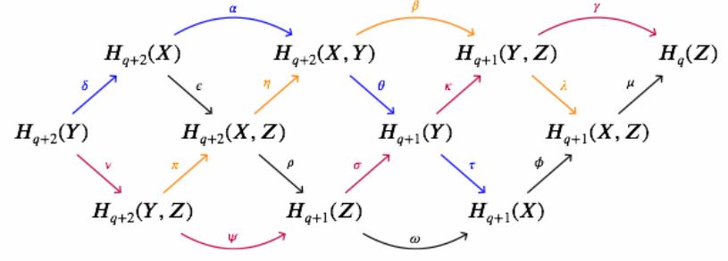
(graphics from this Maths.SE comment, showing the dual situation for homology)

See here for details.

Remark

The exact sequence of a triple in prop. is what gives rise to the Cartan-Eilenberg spectral sequence for $E$-cohomology of a CW-complex $X$.

Example

For $(X,x)$ a pointed topological space and $Cone(X) = (X \wedge (I_+))/X$ its reduced cone, the long exact sequence of the triple $(\{x\}, X, Cone(X))$, prop. ,

$$0 \simeq E^q(Cone(X), \{x\}) \longrightarrow E^q(X,\{x\}) \overset{\bar \delta}{\longrightarrow} E^{q+1}(Cone(X),X) \longrightarrow E^{q+1}(Cone(X), \{x\}) \simeq 0$$

exhibits the connecting homomorphism $\bar \delta$ here as an isomorphism

$$\bar \delta \;\colon\; E^q(X,\{x\}) \overset{\simeq}{\longrightarrow} E^{q+1}(Cone(X),X) \,.$$

This is the suspension isomorphism extracted from the unreduced cohomology theory, see def. below.

Proposition

(Mayer-Vietoris sequence)

Given $E^\bullet$ an unreduced cohomology theory, def. . Given a topological space covered by the interior of two spaces as $X = Int(A) \cup Int(B)$, then for each $C \subset A \cap B$ there is a long exact sequence of cohomology groups of the form

$$\cdots \to E^{n-1}(A \cap B , C) \overset{\bar \delta}{\longrightarrow} E^n(X,C) \longrightarrow E^n(A,C) \oplus E^n(B,C) \longrightarrow E^n(A \cap B, C) \to \cdots \,.$$

e.g. (Switzer 75, theorem 7.19, Aguilar-Gitler-Prieto 02, theorem 12.1.22)

Relation between unreduced and reduced cohomology

Definition

(unreduced to reduced cohomology)

Let $E^\bullet$ be an unreduced cohomology theory, def. . Define a reduced cohomology theory, def. $(\tilde E^\bullet, \sigma)$ as follows.

For $x \colon \ast \to X$ a pointed topological space, set

$$\tilde E^\bullet(X,x) \coloneqq E^\bullet(X,\{x\}) \,.$$

This is clearly functorial. Take the suspension isomorphism to be the composite

$$\sigma \;\colon\; \tilde E^{\bullet+1}(\Sigma X) = E^{\bullet+1}(\Sigma X, \{x\}) \overset{E^\bullet(p)}{\longrightarrow} E^{\bullet+1}(Cone(X),X) \overset{\bar \delta^{-1}}{\longrightarrow} E^\bullet(X,\{x\}) = \tilde E^{\bullet}(X)$$

of the isomorphism $E^\bullet(p)$ from example and the inverse of the isomorphism $\bar \delta$ from example .

Proposition

The construction in def. indeed gives a reduced cohomology theory.

(e.g Switzer 75, 7.34)

Proof

We need to check the exactness axiom given any $A\hookrightarrow X$. By lemma we have an isomorphism

$$\tilde E^\bullet(X \cup Cone(A)) = E^\bullet(X \cup Cone(A), \{\ast\}) \overset{\simeq}{\longrightarrow} E^\bullet(X,A) \,.$$

Unwinding the constructions shows that this makes the following diagram commute:

$$\array{ \tilde E^\bullet(X\cup Cone(A)) &\overset{\simeq}{\longrightarrow}& E^\bullet(X,A) \\ \downarrow && \downarrow \\ \tilde E^\bullet(X) &=& E^\bullet(X,\{x\}) \\ \downarrow && \downarrow \\ \tilde E^\bullet(A) &=& E^\bullet(A,\{a\}) } \,,$$

where the vertical sequence on the right is exact by prop. . Hence the left vertical sequence is exact.

Definition

(reduced to unreduced cohomology)

Let $(\tilde E^\bullet, \sigma)$ be a reduced cohomology theory, def. . Define an unreduced cohomolog theory $E^\bullet$, def. , by

$$E^\bullet(X,A) \coloneqq \tilde E^\bullet( X_+ \cup Cone(A_+))$$

and let the connecting homomorphism be as in def. .

Proposition

The construction in def. indeed yields an unreduced cohomology theory.

e.g. (Switzer 75, 7.35)

Proof

Exactness holds by prop. . For excision, it is sufficient to consider the alternative formulation of lemma . For CW-inclusions, this follows immediately with lemma .

Theorem

The constructions of def. and def. constitute a pair of functors between then categories of reduced cohomology theories, def. and unreduced cohomology theories, def. which exhbit an equivalence of categories.

Proof

(…careful with checking the respect for suspension iso and connecting homomorphism..)

To see that there are natural isomorphisms relating the two composites of these two functors to the identity:

One composite is

$$\begin{aligned} E^\bullet & \mapsto (\tilde E^\bullet \colon (X,x) \mapsto E^\bullet(X,\{x\})) \\ & \mapsto ((E')^\bullet \colon (X,A) \mapsto E^\bullet( X_+ \cup Cone(A_+) ), \ast) \end{aligned} \,,$$

where on the right we have, from the construction, the reduced mapping cone of the original inclusion $A \hookrightarrow X$ with a base point adjoined. That however is isomorphic to the unreduced mapping cone of the original inclusion (prop.- P#UnreducedMappingConeAsReducedConeOfBasedPointAdjoined)). With this the natural isomorphism is given by lemma .

The other composite is

$$\begin{aligned} \tilde E^\bullet & \mapsto (E^\bullet \colon (X,A) \mapsto \tilde E^\bullet(X_+ \cup Cone(A_+))) \\ & \mapsto ((\tilde E')^\bullet \colon X \mapsto \tilde E^\bullet(X_+ \cup Cone(*_+))) \end{aligned}$$

where on the right we have the reduced mapping cone of the point inclusion with a point adoined. As before, this is isomorphic to the unreduced mapping cone of the point inclusion. That finally is clearly homotopy equivalent to $X$, and so now the natural isomorphism follows with homotopy invariance.

Finally we record the following basic relation between reduced and unreduced cohomology:

Proposition

Let $E^\bullet$ be an unreduced cohomology theory, and $\tilde E^\bullet$ its reduced cohomology theory from def. . For $(X,\ast)$ a pointed topological space, then there is an identification

$$E^\bullet(X) \simeq \tilde E^\bullet(X) \oplus E^\bullet(\ast)$$

of the unreduced cohomology of $X$ with the direct sum of the reduced cohomology of $X$ and the unreduced cohomology of the base point.

Proof

The pair $\ast \hookrightarrow X$ induces the sequence

$$\cdots \to E^{\bullet-1}(\ast) \stackrel{\delta}{\longrightarrow} \tilde E^\bullet(X) \stackrel{}{\longrightarrow} E^\bullet(X) \stackrel{}{\longrightarrow} E^\bullet(\ast) \stackrel{\delta}{\longrightarrow} \tilde E^{\bullet+1}(X) \to \cdots$$

which by the exactness clause in def. is exact.

Now since the composite $\ast \to X \to \ast$ is the identity, the morphism $E^\bullet(X) \to E^\bullet(\ast)$ has a section and so is in particular an epimorphism. Therefore, by exactness, the connecting homomorphism vanishes, $\delta = 0$ and we have a short exact sequence

$$0 \to \tilde E^\bullet(X) \stackrel{}{\longrightarrow} E^\bullet(X) \stackrel{}{\longrightarrow} E^\bullet(\ast) \to 0$$

with the right map an epimorphism. Hence this is a split exact sequence and the statement follows.

Generalized homology functors

All of the above has a dual version with generalized cohomology replaced by generalized homology. For ease of reference, we record these dual definitions:

Definition

A reduced homology theory is a functor

$$\tilde E_\bullet \;\colon\; (Top^{\ast/}_{CW}) \longrightarrow Ab^{\mathbb{Z}}$$

from the category of pointed topological spaces (CW-complexes) to $\mathbb{Z}$-graded abelian groups (“homology groups”), in components

$$\tilde E _\bullet \;\colon\; (X \stackrel{f}{\longrightarrow} Y) \mapsto (\tilde E_\bullet(X) \stackrel{f_\ast}{\longrightarrow} \tilde E_\bullet(Y)) \,,$$

and equipped with a natural isomorphism of degree +1, to be called the suspension isomorphism, of the form

$$\sigma \;\colon\; \tilde E_\bullet(-) \overset{\simeq}{\longrightarrow} \tilde E_{\bullet +1}(\Sigma -)$$

such that:

1. (homotopy invariance) If $f_1,f_2 \colon X \longrightarrow Y$ are two morphisms of pointed topological spaces such that there is a (base point preserving) homotopy $f_1 \simeq f_2$ between them, then the induced homomorphisms of abelian groups are equal

   $$f_1_\ast = f_2_\ast \,.$$

2. (exactness) For $i \colon A \hookrightarrow X$ an inclusion of pointed topological spaces, with $j \colon X \longrightarrow Cone(i)$ the induced mapping cone, then this gives an exact sequence of graded abelian groups

   $$\tilde E_\bullet(A) \overset{i_\ast}{\longrightarrow} \tilde E_\bullet(X) \overset{j_\ast}{\longrightarrow} \tilde E_\bullet(Cone(i)) \,.$$

We say $\tilde E_\bullet$ is additive if in addition

• (wedge axiom) For $\{X_i\}_{i \in I}$ any set of pointed CW-complexes, then the canonical morphism

  $$\oplus_{i \in I} \tilde E_\bullet(X_i) \longrightarrow \tilde E^\bullet(\vee_{i \in I} X_i)$$

  from the direct sum of the value on the summands to the value on the wedge sum (prop.- P#WedgeSumAsCoproduct)), is an isomorphism.

We say $\tilde E_\bullet$ is ordinary if its value on the 0-sphere $S^0$ is concentrated in degree 0:

• (Dimension) $\tilde E_{\bullet\neq 0}(\mathbb{S}^0) \simeq 0$.

A homomorphism of reduced cohomology theories

$$\eta \;\colon\; \tilde E_\bullet \longrightarrow \tilde F_\bullet$$

is a natural transformation between the underlying functors which is compatible with the suspension isomorphisms in that all the following squares commute

$$\array{ \tilde E_\bullet(X) &\overset{\eta_X}{\longrightarrow}& \tilde F_\bullet(X) \\ {}^{\mathllap{\sigma_E}}\downarrow && \downarrow^{\mathrlap{\sigma_F}} \\ \tilde E_{\bullet + 1}(\Sigma X) &\overset{\eta_{\Sigma X}}{\longrightarrow}& \tilde F_{\bullet + 1}(\Sigma X) } \,.$$

Definition

A homology theory (unreduced, relative) is a functor

$$E_\bullet : (Top_{CW}^{\hookrightarrow}) \longrightarrow Ab^{\mathbb{Z}}$$

to the category of $\mathbb{Z}$-graded abelian groups, as well as a natural transformation of degree +1, to be called the connecting homomorphism, of the form

$$\delta_{(X,A)} \;\colon\; E_{\bullet + 1}(X, A) \longrightarrow E^\bullet(A, \emptyset) \,.$$

such that:

1. (homotopy invariance) For $f \colon (X_1,A_1) \to (X_2,A_2)$ a homotopy equivalence of pairs, then

   $$E_\bullet(f) \;\colon\; E_\bullet(X_1,A_1) \stackrel{\simeq}{\longrightarrow} E_\bullet(X_2,A_2)$$

   is an isomorphism;

2. (exactness) For $A \hookrightarrow X$ the induced sequence

   $$\cdots \to E_{n+1}(X, A) \stackrel{\delta}{\longrightarrow} E_n(A) \longrightarrow E_n(X) \longrightarrow E_n(X, A) \to \cdots$$

   is a long exact sequence of abelian groups.

(see at long exact sequence in generalized homology)

1. (excision) For $U \hookrightarrow A \hookrightarrow X$ such that $\overline{U} \subset Int(A)$, then the natural inclusion of the pair $i \colon (X-U, A-U) \hookrightarrow (X, A)$ induces an isomorphism

   $$E_\bullet(i) \;\colon\; E_n(X-U, A-U) \overset{\simeq}{\longrightarrow} E_n(X, A)$$

We say $E^\bullet$ is additive if it takes coproducts to direct sums:

• (additivity) If $(X, A) = \coprod_i (X_i, A_i)$ is a coproduct, then the canonical comparison morphism

  $$\oplus_i E^n(X_i, A_i) \overset{\simeq}{\longrightarrow} E^n(X, A)$$

  is an isomorphismfrom the direct sum of the value on the summands, to the value on the total pair.

We say $E_\bullet$ is ordinary if its value on the point is concentrated in degree 0

• (Dimension): $E_{\bullet \neq 0}(\ast,\emptyset) = 0$.

A homomorphism of unreduced homology theories

$$\eta \;\colon\; E_\bullet \longrightarrow F_\bullet$$

is a natural transformation of the underlying functors that is compatible with the connecting homomorphisms, hence such that all these squares commute:

$$\array{ E_{\bullet +1}(X,A) &\overset{\eta_{(X,A)}}{\longrightarrow}& F_{\bullet +1}(X,A) \\ {}^{\mathllap{\delta_E}}\downarrow && \downarrow^{\mathrlap{\delta_F}} \\ E_\bullet(A,\emptyset) &\overset{\eta_{(A,\emptyset)}}{\longrightarrow}& F^\bullet(A,\emptyset) } \,.$$

Multiplicative cohomology theories

The generalized cohomology theories considered above assign cohomology groups. It is familiar from ordinary cohomology with coefficients not just in a group but in a ring, that also the cohomology groups inherit compatible ring structure. The generalization of this phenomenon to generalized cohomology theories is captured by the concept of multiplicative cohomology theories:

Definition

Let $E_1, E_2, E_3$ be three unreduced generalized cohomology theories (def.). A pairing of cohomology theories

$$\mu \;\colon\; E_1 \Box E_2 \longrightarrow E_3$$

is a natural transformation (of functors on $(Top_{CW}^{\hookrightarrow}\times Top_{CW}^{\hookrightarrow})^{op}$) of the form

$$\mu_{n_1,n_2} \;\colon\; E_1^{n_1}(X,A) \otimes E_2^{n_2}(Y,B) \longrightarrow E_3^{n_1 + n_2}(X\times Y \;,\; A\times Y \cup X \times B)$$

such that this is compatible with the connecting homomorphisms $\delta_i$ of $E_i$, in that the following are commuting squares

$$\array{ E_1^{n_1}(A) \otimes E_2^{n_2}(Y,B) &\overset{\delta_1 \otimes id_2}{\longrightarrow}& E_1^{n_1+1}(X,A) \otimes E_2^{n_2}(Y,B) \\ {}^{\mathllap{\mu_{n_1,n_2}}}\downarrow && \downarrow^{\mathrlap{\mu_{n_1+1, n_2}}} \\ \underoverset {E_3^{n_1 + n_2}(A \times Y \cup X \times B , X \times B)} {E_3^{n_1 + n_2}(A \times Y, A \times B)} {\simeq} &\overset{\delta_3}{\longrightarrow}& E_3^{n_1 + n_2+ 1}(X \times Y, A \times B) }$$

and

$$\array{ E_1^{n_1}(X,A) \otimes E_2^{n_2}(B) &\overset{(-1)^{n_1} id_1 \otimes \delta_2}{\longrightarrow}& E_1^{n_1+1}(X,A) \otimes E_2^{n_2}(Y,B) \\ {}^{\mathllap{\mu_{n_1,n_2}}}\downarrow && \downarrow^{\mathrlap{\mu_{n_1, n_2 + 1}}} \\ \underoverset {E_3^{n_1 + n_2}(A \times Y \cup X \times B , A \times Y)} {E_3^{n_1 + n_2}(X \times B, A \times B)} {\simeq} &\overset{\delta_3}{\longrightarrow}& E_3^{n_1 + n_2+ 1}(X \times Y, A \times B) } \,,$$

where the isomorphisms in the bottom left are the excision isomorphisms.

Definition

An (unreduced) multiplicative cohomology theory is an unreduced generalized cohomology theory theory $E$ (def. ) equipped with

1. (external multiplication) a pairing (def. ) of the form $\mu \;\colon\; E \Box E \longrightarrow E$;

2. (unit) an element $1 \in E^0(\ast)$

such that

1. (associativity) $\mu \circ (id \otimes \mu) = \mu \circ (\mu \otimes id)$;

2. (unitality) $\mu(1\otimes x) = \mu(x \otimes 1) = x$ for all $x \in E^n(X,A)$.

The mulitplicative cohomology theory is called commutative (often considered by default) if in addition

• (graded commutativity)

  $$\array{ E^{n_1}(X,A) \otimes E^{n_2}(Y,B) &\overset{(u \otimes v) \mapsto (-1)^{n_1 n_2} (v \otimes u) }{\longrightarrow}& E^{n_2}(Y,B) \otimes E^{n_1}_{X,A} \\ {}^{\mathllap{\mu_{n_1,n_2}}}\downarrow && \downarrow^{\mathrlap{\mu_{n_2,n_1}}} \\ E^{n_1 + n_2}( X \times Y , A \times Y \cup X \times B) &\underset{(switch_{(X,A), (Y,B)})^\ast}{\longrightarrow}& E^{n_1 + n_2}( Y \times X , B \times X \cup Y \times A) } \,.$$

Given a multiplicative cohomology theory $(E, \mu, 1)$, its cup product is the composite of the above external multiplication with pullback along the diagonal maps $\Delta_{(X,A)} \colon (X,A) \longrightarrow (X\times X, A \times X \cup X \times A)$;

$$(-) \cup (-) \;\colon\; E^{n_1}(X,A) \otimes E^{n_2}(X,A) \overset{\mu_{n_1,n_2}}{\longrightarrow} E^{n_1 + n_2}( X \times X, \; A \times X \cup X \times A) \overset{\Delta^\ast_{(X,A)}}{\longrightarrow} E^{n_1 + n_2}(X, \; A \cup B) \,.$$

e.g. (Tamaki-Kono 06, II.6)

Proposition

Let $(E,\mu,1)$ be a multiplicative cohomology theory, def. . Then

1. For every space $X$ the cup product gives $E^\bullet(X)$ the structure of a $\mathbb{Z}$-graded ring, which is graded-commutative if $(E,\mu,1)$ is commutative.

2. For every pair $(X,A)$ the external multiplication $\mu$ gives $E^\bullet(X,A)$ the structure of a left and right module over the graded ring $E^\bullet(\ast)$.

3. All pullback morphisms respect the left and right action of $E^\bullet(\ast)$ and the connecting homomorphisms respect the right action and the left action up to multiplication by $(-1)^{n_1}$

Proof

Regarding the third point:

For pullback maps this is the naturality of the external product: let $f \colon (X,A) \longrightarrow (Y,B)$ be a morphism in $Top_{CW}^{\hookrightarrow}$ then naturality says that the following square commutes:

$$\array{ E^{n_1}(\ast) \otimes E^{n_2}(Y,B) &\overset{\mu_{n_1,n_2}}{\longrightarrow}& E^{n_1 + n_2}(Y, B) \\ {}^{\mathllap{(id,f^\ast)}}\downarrow && \downarrow^{\mathrlap{f^\ast}} \\ E^{n_1}(\ast) \otimes E^{n_2}(X,A) &\overset{\mu_{n_1,n_2}}{\longrightarrow}& E^{n_1 + n_2}(Y,B) } \,.$$

For connecting homomorphisms this is the (graded) commutativity of the squares in def. :

$$\array{ E^{n_1}(\ast)\otimes E^{n_2}(A) &\overset{(-1)^{n_1} (id, \delta)}{\longrightarrow}& E^{n_1}(\ast) \otimes E^{n_2 + 2}(X) \\ {}^{\mathllap{\mu_{n_1,n_2}}}\downarrow && \downarrow^{\mathrlap{\mu_{n_1,n_2}}} \\ E^{n_1 + n_2}(A) &\overset{\delta}{\longrightarrow}& E_3^{n_1 + n_2+ 1}(X,B) } \,.$$

Brown representability theorem

Idea. Given any functor such as the generalized (co)homology functor above, an important question to ask is whether it is a representable functor. Due to the $\mathbb{Z}$-grading and the suspension isomorphisms, if a generalized (co)homology functor is representable at all, it must be represented by a $\mathbb{Z}$-indexed sequence of pointed topological spaces such that the reduced suspension of one is comparable to the next one in the list. This is a spectrum or more specifically: a sequential spectrum .

Whitehead observed that indeed every spectrum represents a generalized (co)homology theory. The Brown representability theorem states that, conversely, every generalized (co)homology theory is represented by a spectrum, subject to conditions of additivity.

As a first application, Eilenberg-MacLane spectra representing ordinary cohomology may be characterized via Brown representability.

Literature. (Switzer 75, section 9, Aguilar-Gitler-Prieto 02, section 12, Kochman 96, 3.4)

Traditional discussion

Write $Top_{{\geq 1}}^{\ast/} \hookrightarrow Top^{\ast/}$ for the full subcategory of connected pointed topological spaces. Write $Set^{\ast/}$ for the category of pointed sets.

Definition

A Brown functor is a functor

$$F\;\colon \; Ho(Top_{\geq 1}^{\ast/})^{op} \longrightarrow Set^{\ast/}$$

(from the opposite of the classical homotopy category (def., def.) of connected pointed topological spaces) such that

1. (additivity) $F$ takes small coproducts (wedge sums) to products;

2. (Mayer-Vietoris) If $X = Int(A) \cup Int(B)$ then for all $x_A \in F(A)$ and $x_B \in F(B)$ such that $(x_A)|_{A \cap B} = (x_B)|_{A \cap B}$ then there exists $x_X \in F(X)$ such that $x_A = (x_X)|_A$ and $x_B = (x_X)|_B$.

Proposition

For every additive reduced cohomology theory $\tilde E^\bullet(-) \colon Ho(Top^{\ast/})^{op}\to Set^{\ast/}$ (def. ) and for each degree $n \in \mathbb{N}$, the restriction of $\tilde E^n(-)$ to connected spaces is a Brown functor (def. ).

Proof

Under the relation between reduced and unreduced cohomology above, this follows from the exactness of the Mayer-Vietoris sequence of prop. .

Theorem

(Brown representability)

Every Brown functor $F$ (def. ) is representable, hence there exists $X \in Top_{\geq 1}^{\ast/}$ and a natural isomorphism

$$[-,X]_{\ast} \overset{\simeq}{\longrightarrow} F(-)$$

(where $[-,-]_\ast$ denotes the hom-functor of $Ho(Top_{\geq 1}^{\ast/})$ (exmpl.)).

(e.g. AGP 02, theorem 12.2.22)

Remark

A key subtlety in theorem is the restriction to connected pointed topological spaces in def. . This comes about since the proof of the theorem requires that continuous functions $f \colon X \longrightarrow Y$ that induce isomorphisms on pointed homotopy classes

$$[S^n,X]_\ast \longrightarrow [S^n,Y]_\ast$$

for all $n$ are weak homotopy equivalences (For instance in AGP 02 this is used in the proof of theorem 12.2.19 there). But $[S^n,X]_\ast = \pi_n(X,x)$ gives the $n$th homotopy group of $X$ only for the canonical basepoint, while for a weak homotopy equivalence in general one needs to consider the homotopy groups at all possible basepoints, at least one for each connected component. But so if one does assume that all spaces involved are connected, hence only have one connected component, then indeed weak homotopy equivalences are equivalently those maps $X\to Y$ making all the $[S^n,X]_\ast \longrightarrow [S^n,Y]_\ast$ into isomorphisms.

See also example below.

The representability result applied degreewise to an additive reduced cohomology theory will yield (prop. below) the following concept.

Definition

An Omega-spectrum $X$ (def.) is

1. a sequence $\{X_n\}_{n \in \mathbb{N}}$ of pointed topological spaces $X_n \in Top^{\ast/}$

2. weak homotopy equivalences

   $$\tilde \sigma_n \;\colon\; X_n \underoverset{\in W_{cl}}{\tilde \sigma_n}{\longrightarrow} \Omega X_{n+1}$$

   for each $n \in \mathbb{N}$, form each space to the loop space of the following space.

Proposition

Every additive reduced cohomology theory $\tilde E^\bullet(-) \colon (Top_{CW}^\ast)^{op} \longrightarrow Ab^{\mathbb{Z}}$ according to def. , is represented by an Omega-spectrum $E$ (def. ) in that in each degree $n \in \mathbb{N}$

1. $\tilde E^n(-)$ is represented by some $E_n \in Ho(Top^{\ast/})$;

2. the suspension isomorphism $\sigma_n$ of $\tilde E^\bullet$ is represented by the structure map $\tilde \sigma_n$ of the Omega-spectrum in that for all $X \in Top^{\ast/}$ the following diagram commutes:

   $$\array{ \tilde E^{n}(X) &\overset{\sigma_n(X)}{\longrightarrow}& &\longrightarrow& \tilde E^{n+1}(\Sigma X) \\ {}^{\mathllap{\simeq}}\downarrow && && \downarrow^{\mathrlap{\simeq}} \\ [X,E_n]_\ast &\overset{[X,\tilde \sigma_n]_\ast}{\longrightarrow}& [X, \Omega E_{n+1}]_\ast &\simeq& [\Sigma X, E_{n+1}]_\ast } \,,$$

   where $[-,-]_\ast \coloneqq Hom_{Ho(Top_{\geq 1}^{\ast/})}$ denotes the hom-sets in the classical pointed homotopy category (def.) and where in the bottom right we have the $(\Sigma\dashv \Omega)$-adjunction isomorphism (prop.).

Proof

If it were not for the connectedness clause in def. (remark ), then theorem with prop. would immediately give the existence of the $\{E_n\}_{n \in \mathbb{N}}$ and the remaining statement would follow immediately with the Yoneda lemma, which says in particular that morphisms between representable functors are in natural bijection with the morphisms of objects that represent them.

The argument with the connectivity condition in Brown representability taken into account is essentially the same, just with a little bit more care:

For $X$ a pointed topological space, write $X^{(0)}$ for the connected component of its basepoint. Observe that the loop space of a pointed topological space only depends on this connected component:

$$\Omega X \simeq \Omega (X^{(0)}) \,.$$

Now for $n \in \mathbb{N}$, to show that $\tilde E^n(-)$ is representable by some $E_n \in Ho(Top^{\ast/})$, use first that the restriction of $\tilde E^{n+1}$ to connected spaces is represented by some $E_{n+1}^{(0)}$. Observe that the reduced suspension of any $X \in Top^{\ast/}$ lands in $Top_{\geq 1}^{\ast/}$. Therefore the $(\Sigma\dashv \Omega)$-adjunction isomorphism (prop.) implies that $\tilde E^{n+1}(\Sigma(-))$ is represented on all of $Top^{\ast/}$ by $\Omega E_{n+1}^{(0)}$:

$$\tilde E^{n+1}(\Sigma X) \simeq [\Sigma X, E_{n+1}^{(0)}]_\ast \simeq [X, \Omega E_{n+1}^{(0)}]_\ast \simeq [X, \Omega E_{n+1}]_\ast \,,$$

where $E_{n+1}$ is any pointed topological space with the given connected component $E_{n+1}^{(0)}$.

Now the suspension isomorphism of $\tilde E$ says that $E_n \in Ho(Top^{\ast/})$ representing $\tilde E^n$ exists and is given by $\Omega E_{n+1}^{(0)}$:

$$\tilde E^n(X) \simeq \tilde E^{n+1}(\Sigma, X)\simeq [X,\Omega E_{n+1}]$$

for any $E_{n+1}$ with connected component $E_{n+1}^{(0)}$.

This completes the proof. Notice that running the same argument next for $(n+1)$ gives a representing space $E_{n+1}$ such that its connected component of the base point is $E_{n+1}^{(0)}$ found before. And so on.

Conversely:

Proposition

Every Omega-spectrum $E$, def. , represents an additive reduced cohomology theory def. $\tilde E^\bullet$ by

$$\tilde E^n(X) \coloneqq [X,E_n]_\ast$$

with suspension isomorphism given by

$$\sigma_n \;\colon\; \tilde E^n(X) = [X,E_n]_\ast \overset{[X,\tilde \sigma_n]}{\longrightarrow} [X, \Omega E_{n+1}]_\ast \overset{\simeq}{\to} [\Sigma X, E_{n+1}] = \tilde E^{n+1}(\Sigma X) \,.$$

Proof

The additivity is immediate from the construction. The exactnes follows from the long exact sequences of homotopy cofiber sequences given by this prop..

Remark

If we consider the stable homotopy category $Ho(Spectra)$ of spectra (def.) and consider any topological space $X$ in terms of its suspension spectrum $\Sigma^\infty X \in Ho(Spectra)$ (exmpl.), then the statement of prop. is more succinctly summarized by saying that the graded reduced cohomology groups of a topological space $X$ represented by an Omega-spectrum $E$ are the hom-groups

$$\tilde E^\bullet(X) \;\simeq\; [\Sigma^\infty X, \Sigma^\bullet E]$$

in the stable homotopy category, into all the suspensions (thm.) of $E$.

This means that more generally, for $X \in Ho(Spectra)$ any spectrum, it makes sense to consider

$$\tilde E^\bullet(X) \;\coloneqq\; [X,\Sigma^\bullet E]$$

to be the graded reduced generalized $E$-cohomology groups of the spectrum $X$.

See also in part 1 this example.

Application to ordinary cohomology

Example

Let $A$ be an abelian group. Consider singular cohomology $H^n(-,A)$ with coefficients in $A$. The corresponding reduced cohomology evaluated on n-spheres satisfies

$$\tilde H^n(S^q,A) \simeq \left\{ \array{ A & if \; q = n \\ 0 & otherwise } \right.$$

Hence singular cohomology is a generalized cohomology theory which is “ordinary cohomology” in the sense of def. .

Applying the Brown representability theorem as in prop. hence produces an Omega-spectrum (def. ) whose $n$th component space is characterized as having homotopy groups concentrated in degree $n$ on $A$. These are called Eilenberg-MacLane spaces $K(A,n)$

$$\pi_q(K(A,n)) \simeq \left\{ \array{ A & if \; q = n \\ 0 & otherwise } \right. \,.$$

Here for $n \gt 0$ then $K(A,n)$ is connected, therefore with an essentially unique basepoint, while $K(A,0)$ is (homotopy equivalent to) the underlying set of the group $A$.

Such spectra are called Eilenberg-MacLane spectra $H A$:

$$(H A)_n \simeq K(A,n) \,.$$

As a consequence of example one obtains the uniqueness result of Eilenberg-Steenrod:

Proposition

Let $\tilde E_1$ and $\tilde E_2$ be ordinary (def. ) generalized (Eilenberg-Steenrod) cohomology theories. If there is an isomorphism

$$\tilde E_1(S^0) \simeq \tilde E_2(S^0)$$

of cohomology groups of the 0-sphere, then there is an isomorphism of cohomology theories

$$\tilde E_1 \overset{\simeq}{\longrightarrow} \tilde E_2 \,.$$

(e.g. Aguilar-Gitler-Prieto 02, theorem 12.3.6)

Homotopy-theoretic discussion

Using abstract homotopy theory in the guise of model category theory (see the lecture notes on classical homotopy theory), the traditional proof and further discussion of the Brown representability theorem above becomes more transparent (Lurie 10, section 1.4.1, for exposition see also Mathew 11).

This abstract homotopy-theoretic proof uses the general concept of homotopy colimits in model categories as well as the concept of derived hom-spaces (“∞-categories”). Even though in the accompanying Lecture notes on classical homotopy theory these concepts are only briefly indicated, the following is included for the interested reader.

Definition

Let $\mathcal{C}$ be a model category. A functor

$$F \;\colon\; Ho(\mathcal{C})^{op} \longrightarrow Set$$

(from the opposite of the homotopy category of $\mathcal{C}$ to Set)

is called a Brown functor if

1. it sends small coproducts to products;

2. it sends homotopy pushouts in $\mathcal{C}\to Ho(\mathcal{C})$ to weak pullbacks in Set (see remark ).

Remark

A weak pullback is a diagram that satisfies the existence clause of a pullback, but not necessarily the uniqueness condition. Hence the second clause in def. says that for a homotopy pushout square

$$\array{ Z &\longrightarrow& X \\ \downarrow &\swArrow& \downarrow \\ Y &\longrightarrow& X \underset{Z}{\sqcup}Y }$$

in $\mathcal{C}$, then the induced universal morphism

$$F\left(X \underset{Z}{\sqcup}Y\right) \stackrel{epi}{\longrightarrow} F(X) \underset{F(Z)}{\times} F(Y)$$

into the actual pullback is an epimorphism.

Definition

Say that a model category $\mathcal{C}$ is compactly generated by cogroup objects closed under suspensions if

1. $\mathcal{C}$ is generated by a set

   $$\{S_i \in \mathcal{C}\}_{i \in I}$$

   of compact objects (i.e. every object of $\mathcal{C}$ is a homotopy colimit of the objects $S_i$.)

2. each $S_i$ admits the structure of a cogroup object in the homotopy category $Ho(\mathcal{C})$;

3. the set $\{S_i\}$ is closed under forming reduced suspensions.

Example

(suspensions are H-cogroup objects)

Let $\mathcal{C}$ be a model category and $\mathcal{C}^{\ast/}$ its pointed model category (prop.) with zero object (rmk.). Write $\Sigma \colon X \mapsto 0 \underset{X}{\coprod} 0$ for the reduced suspension functor.

Then the fold map

$$\Sigma X \coprod \Sigma X \simeq 0 \underset{X}{\sqcup} 0 \underset{X}{\sqcup} 0 \longrightarrow 0 \underset{X}{\sqcup} X \underset{X}{\sqcup} 0 \simeq 0 \underset{X}{\sqcup} 0 \simeq \Sigma X$$

exhibits cogroup structure on the image of any suspension object $\Sigma X$ in the homotopy category.

This is equivalently the group-structure of the first (fundamental) homotopy group of the values of functor co-represented by $\Sigma X$:

$$Ho(\mathcal{C})(\Sigma X, -) \;\colon\; Y \mapsto Ho(\mathcal{C})(\Sigma X, Y) \simeq Ho(\mathcal{C})(X, \Omega Y) \simeq \pi_1 Ho(\mathcal{C})(X, Y) \,.$$

Example

In bare pointed homotopy types $\mathcal{C} = Top^{\ast/}_{Quillen}$, the (homotopy types of) n-spheres $S^n$ are cogroup objects for $n \geq 1$, but not for $n = 0$, by example . And of course they are compact objects.

So while $\{S^n\}_{n \in \mathbb{N}}$ generates all of the homotopy theory of $Top^{\ast/}$, the latter is not an example of def. due to the failure of $S^0$ to have cogroup structure.

Removing that generator, the homotopy theory generated by $\{S^n\}_{{n \in \mathbb{N}} \atop {n \geq 1}}$ is $Top^{\ast/}_{\geq 1}$, that of connected pointed homotopy types. This is one way to see how the connectedness condition in the classical version of Brown representability theorem arises. See also remark above.

See also (Lurie 10, example 1.4.1.4)

In homotopy theories compactly generated by cogroup objects closed under forming suspensions, the following strenghtening of the Whitehead theorem holds.

Proposition

In a homotopy theory compactly generated by cogroup objects $\{S_i\}_{i \in I}$ closed under forming suspensions, according to def. , a morphism $f\colon X \longrightarrow Y$ is an equivalence precisely if for each $i \in I$ the induced function of maps in the homotopy category

$$Ho(\mathcal{C})(S_i,f) \;\colon\; Ho(\mathcal{C})(S_i,X) \longrightarrow Ho(\mathcal{C})(S_i,Y)$$

is an isomorphism (a bijection).

(Lurie 10, p. 114, Lemma star)

Proof

By the ∞-Yoneda lemma, the morphism $f$ is a weak equivalence precisely if for all objects $A \in \mathcal{C}$ the induced morphism of derived hom-spaces

$$\mathcal{C}(A,f) \;\colon\; \mathcal{C}(A,X) \longrightarrow \mathcal{C}(A,Y)$$

is an equivalence in $Top_{Quillen}$. By assumption of compact generation and since the hom-functor $\mathcal{C}(-,-)$ sends homotopy colimits in the first argument to homotopy limits, this is the case precisely already if it is the case for $A \in \{S_i\}_{i \in I}$.

Now the maps

$$\mathcal{C}(S_i,f) \;\colon\; \mathcal{C}(S_i,X) \longrightarrow \mathcal{C}(S_i,Y)$$

are weak equivalences in $Top_{Quillen}$ if they are weak homotopy equivalences, hence if they induce isomorphisms on all homotopy groups $\pi_n$ for all basepoints.

It is this last condition of testing on all basepoints that the assumed cogroup structure on the $S_i$ allows to do away with: this cogroup structure implies that $\mathcal{C}(S_i,-)$ has the structure of an $H$-group, and this implies (by group multiplication), that all connected components have the same homotopy groups, hence that all homotopy groups are independent of the choice of basepoint, up to isomorphism.

Therefore the above morphisms are equivalences precisely if they are so under applying $\pi_n$ based on the connected component of the zero morphism

$$\pi_n\mathcal{C}(S_i,f) \;\colon\; \pi_n \mathcal{C}(S_i,X) \longrightarrow \pi_n\mathcal{C}(S_i,Y) \,.$$

Now in this pointed situation we may use that

$$\begin{aligned} \pi_n \mathcal{C}(-,-) & \simeq \pi_0 \mathcal{C}(-,\Omega^n(-)) \\ & \simeq \pi_0\mathcal{C}(\Sigma^n(-),-) \\ & \simeq Ho(\mathcal{C})(\Sigma^n(-),-) \end{aligned}$$

to find that $f$ is an equivalence in $\mathcal{C}$ precisely if the induced morphisms

$$Ho(\mathcal{C})(\Sigma^n S_i, f) \;\colon\; Ho(\mathcal{C})(\Sigma^n S_i,X) \longrightarrow Ho(\mathcal{C})(\Sigma^n S_i,Y)$$

are isomorphisms for all $i \in I$ and $n \in \mathbb{N}$.

Finally by the assumption that each suspension $\Sigma^n S_i$ of a generator is itself among the set of generators, the claim follows.

Theorem

(Brown representability)

Let $\mathcal{C}$ be a model category compactly generated by cogroup objects closed under forming suspensions, according to def. . Then a functor

$$F \;\colon\; Ho(\mathcal{C})^{op} \longrightarrow Set$$

(from the opposite of the homotopy category of $\mathcal{C}$ to Set) is representable precisely if it is a Brown functor, def. .

(Lurie 10, theorem 1.4.1.2)

Proof

Due to the version of the Whitehead theorem of prop. we are essentially reduced to showing that Brown functors $F$ are representable on the $S_i$. To that end consider the following lemma. (In the following we notationally identify, via the Yoneda lemma, objects of $\mathcal{C}$, hence of $Ho(\mathcal{C})$, with the functors they represent.)

Lemma ($\star$): Given $X \in \mathcal{C}$ and $\eta \in F(X)$, hence $\eta \colon X \to F$, then there exists a morphism $f \colon X \to X'$ and an extension $\eta' \colon X' \to F$ of $\eta$ which induces for each $S_i$ a bijection $\eta'\circ (-) \colon PSh(Ho(\mathcal{C}))(S_i,X') \stackrel{\simeq}{\longrightarrow} Ho(\mathcal{C})(S_i,F) \simeq F(S_i)$.

To see this, first notice that we may directly find an extension $\eta_0$ along a map $X\to X_o$ such as to make a surjection: simply take $X_0$ to be the coproduct of all possible elements in the codomain and take

$$\eta_0 \;\colon\; X \sqcup \left( \underset{{i \in I,} \atop {\gamma \colon S_i \stackrel{}{\to} F}}{\coprod} S_i \right) \longrightarrow F$$

to be the canonical map. (Using that $F$, by assumption, turns coproducts into products, we may indeed treat the coproduct in $\mathcal{C}$ on the left as the coproduct of the corresponding functors.)

To turn the surjection thus constructed into a bijection, we now successively form quotients of $X_0$. To that end proceed by induction and suppose that $\eta_n \colon X_n \to F$ has been constructed. Then for $i \in I$ let

$$K_i \coloneqq ker \left( Ho(\mathcal{C})(S_i, X_n) \stackrel{\eta_n \circ (-)}{\longrightarrow} F(S_i) \right)$$

be the kernel of $\eta_n$ evaluated on $S_i$. These $K_i$ are the pieces that need to go away in order to make a bijection. Hence define $X_{n+1}$ to be their joint homotopy cofiber

$$X_{n+1} \coloneqq coker\left( \left( \underset{{i \in I,} \atop {\gamma \in K_i}}{\sqcup} S_i \right) \overset{(\gamma)_{{i \in I} \atop {\gamma\in K_i}}}{\longrightarrow} X_n \right) \,.$$

Then by the assumption that $F$ takes this homotopy cokernel to a weak fiber (as in remark ), there exists an extension $\eta_{n+1}$ of $\eta_n$ along $X_n \to X_{n+1}$:

Then by the assumption that $F$ takes this homotopy cokernel to a weak fiber (as in remark ), there exists an extension $\eta_{n+1}$ of $\eta_n$ along $X_n \to X_{n+1}$:

$$\array{ \left( \underset{{i \in I}\atop {\gamma \in K_i}}{\sqcup} S_i \right) &\overset{(\gamma)_{{i \in I}\atop \gamma \in K_i}}{\longrightarrow}& X_n &\overset{\eta_n}{\longrightarrow}& F \\ \downarrow &(po^{h})& \downarrow & \nearrow_{\mathrlap{\exists \eta_{n+1}}} \\ \ast &\longrightarrow& X_{n+1} } \;\;\;\;\;\;\;\;\;\;\; \Leftrightarrow \;\;\;\;\;\;\;\;\;\;\; \array{ && F(X_{n+1}) &\longrightarrow& \ast \\ &{}^{\mathllap{\exists \eta_{n+1}}}\nearrow& \downarrow^{\mathrlap{epi}} && \downarrow \\ \ast &\overset{\eta_n}{\longrightarrow}& ker\left((\gamma^\ast\right)_{{i \in I} \atop {\gamma \in K_i}}) &\longrightarrow& \ast \\ &{}_{\mathllap{\eta_n}}\searrow& \downarrow &(pb)& \downarrow \\ && F(X_n) &\underset{(\gamma^\ast)_{{i \in I} \atop {\gamma \in K_i}} }{\longrightarrow}& \underset{{i \in I}\atop {\gamma\in K_i}}{\prod}F(S_i) } \,.$$

It is now clear that we want to take

$$X' \coloneqq \underset{\rightarrow}{\lim}_n X_n$$

and extend all the $\eta_n$ to that colimit. Since we have no condition for evaluating $F$ on colimits other than pushouts, observe that this sequential colimit is equivalent to the following pushout:

$$\array{ \underset{n}{\sqcup} X_n &\longrightarrow& \underset{n}{\sqcup} X_{2n} \\ \downarrow && \downarrow \\ \underset{n}{\sqcup} X_{2n+1} &\longrightarrow& X' } \,,$$

where the components of the top and left map alternate between the identity on $X_n$ and the above successor maps $X_n \to X_{n+1}$. Now the excision property of $F$ applies to this pushout, and we conclude the desired extension $\eta' \colon X' \to F$:

$$\array{ && \underset{n}{\sqcup} X_n \\ & \swarrow && \searrow \\ \underset{n}{\sqcup} X_{2n+1} &\longrightarrow& X' &\longleftarrow& \underset{n}{\sqcup} X_{2n} \\ & {}_{\mathllap{(\eta_{2n+1})_{n}}}\searrow& \downarrow^{\mathrlap{\exists \eta}} & \swarrow_{\mathrlap{(\eta_{2n})_n}} \\ && F } \;\;\;\;\;\;\;\;\; \Leftrightarrow \;\;\;\;\;\;\;\;\; \array{ && F(X') \\ &{}^{\mathllap{\exists \eta}}\nearrow& \downarrow^{\mathrlap{epi}} \\ &\ast \overset{(\eta_n)_n}{\longrightarrow}& \underset{\longleftarrow}{\lim}_n F(X_n) \\ & \swarrow && \searrow \\ \underset{n}{\prod}F(X_{2n+1}) && && \underset{n}{\prod}(X_{2n}) \\ & \searrow && \swarrow \\ && \underset{n}{\prod}F(X_n) } \,,$$

It remains to confirm that this indeed gives the desired bijection. Surjectivity is clear. For injectivity use that all the $S_i$ are, by assumption, compact, hence they may be taken inside the sequential colimit:

$$\array{ && X_{n(\gamma)} \\ &{}^{\mathllap{ \exists \hat \gamma}}\nearrow& \downarrow \\ S_i &\overset{\gamma}{\longrightarrow}& X' = \underset{\longrightarrow}{\lim}_n X_n } \,.$$

With this, injectivity follows because by construction we quotiented out the kernel at each stage. Because suppose that $\gamma$ is taken to zero in $F(S_i)$, then by the definition of $X_{n+1}$ above there is a factorization of $\gamma$ through the point:

$$\array{ 0 \colon & S_i &\overset{\hat \gamma}{\longrightarrow}& X_{n(\gamma)} &\overset{\eta_n}{\longrightarrow}& F \\ & \downarrow && \downarrow & \\ & \ast &\longrightarrow& X_{n(\gamma)+1} \\ & && \downarrow \\ & && X' }$$

This concludes the proof of Lemma ($\star$).

Now apply the construction given by this lemma to the case $X_0 \coloneqq 0$ and the unique $\eta_0 \colon 0 \stackrel{\exists !}{\to} F$. Lemma $(\star)$ then produces an object $X'$ which represents $F$ on all the $S_i$, and we want to show that this $X'$ actually represents $F$ generally, hence that for every $Y \in \mathcal{C}$ the function

$$\theta \coloneqq \eta'\circ (-) \;\colon\; Ho(\mathcal{C})(Y,X') \stackrel{}{\longrightarrow} F(Y)$$

is a bijection.

First, to see that $\theta$ is surjective, we need to find a preimage of any $\rho \colon Y \to F$. Applying Lemma $(\star)$ to $(\eta',\rho)\colon X'\sqcup Y \longrightarrow F$ we get an extension $\kappa$ of this through some $X' \sqcup Y \longrightarrow Z$ and the morphism on the right of the following commuting diagram:

$$\array{ Ho(\mathcal{C})(-,X') && \longrightarrow && Ho(\mathcal{C})(-, Z) \\ & {}_{\mathllap{\eta'\circ(-)}}\searrow && \swarrow_{\mathrlap{\kappa \circ (-)}} \\ && F(-) } \,.$$

Moreover, Lemma $(\star)$ gives that evaluated on all $S_i$, the two diagonal morphisms here become isomorphisms. But then prop. implies that $X' \longrightarrow Z$ is in fact an equivalence. Hence the component map $Y \to Z \simeq Z$ is a lift of $\kappa$ through $\theta$.

Second, to see that $\theta$ is injective, suppose $f,g \colon Y \to X'$ have the same image under $\theta$. Then consider their homotopy pushout

$$\array{ Y \sqcup Y &\stackrel{(f,g)}{\longrightarrow}& X' \\ \downarrow && \downarrow \\ Y &\longrightarrow& Z }$$

along the codiagonal of $Y$. Using that $F$ sends this to a weak pullback by assumption, we obtain an extension $\bar \eta$ of $\eta'$ along $X' \to Z$. Applying Lemma $(\star)$ to this gives a further extension $\bar \eta' \colon Z' \to Z$ which now makes the following diagram

$$\array{ Ho(\mathcal{C})(-,X') && \longrightarrow && Ho(\mathcal{C})(-, Z) \\ & {}_{\mathllap{\eta'\circ(-)}}\searrow && \swarrow_{\mathrlap{\bar \eta' \circ (-)}} \\ && F(-) }$$

such that the diagonal maps become isomorphisms when evaluated on the $S_i$. As before, it follows via prop. that the morphism $h \colon X' \longrightarrow Z'$ is an equivalence.

Since by this construction $h\circ f$ and $h\circ g$ are homotopic

$$\array{ Y \sqcup Y &\stackrel{(f,g)}{\longrightarrow}& X' \\ \downarrow && \downarrow & \searrow^{\mathrlap{\stackrel{h}{\simeq}}} \\ Y &\longrightarrow& Z &\longrightarrow& Z' }$$

it follows with $h$ being an equivalence that already $f$ and $g$ were homotopic, hence that they represented the same element.

Proposition

Given a reduced additive cohomology functor $H^\bullet \colon Ho(\mathcal{C})^{op}\to Ab^{\mathbb{Z}}$, def. , its underlying Set-valued functors $H^n \colon Ho(\mathcal{C})^{op}\to Ab\to Set$ are Brown functors, def. .

Proof

The first condition on a Brown functor holds by definition of $H^\bullet$. For the second condition, given a homotopy pushout square

$$\array{ X_1 &\stackrel{f_1}{\longrightarrow}& Y_1 \\ \downarrow^{} && \downarrow \\ X_2 &\stackrel{f_2}{\longrightarrow}& Y_2 }$$

in $\mathcal{C}$, consider the induced morphism of the long exact sequences given by prop.

$$\array{ H^\bullet(coker(f_2)) &\longrightarrow& H^\bullet(Y_2) &\stackrel{f^\ast_2}{\longrightarrow}& H^\bullet(X_2) &\stackrel{}{\longrightarrow}& H^{\bullet+1}(\Sigma coker(f_2)) \\ {}^{\mathllap{\simeq}}\downarrow && \downarrow && \downarrow && \downarrow^{\mathrlap{\simeq}} \\ H^\bullet(coker(f_1)) &\longrightarrow& H^\bullet(Y_1) &\stackrel{f^\ast_1}{\longrightarrow}& H^\bullet(X_1) &\stackrel{}{\longrightarrow}& H^{\bullet+1}(\Sigma coker(f_1)) }$$

Here the outer vertical morphisms are isomorphisms, as shown, due to the pasting law (see also at fiberwise recognition of stable homotopy pushouts). This means that the four lemma applies to this diagram. Inspection shows that this implies the claim.

Corollary

Let $\mathcal{C}$ be a model category which satisfies the conditions of theorem , and let $(H^\bullet, \delta)$ be a reduced additive generalized cohomology functor on $\mathcal{C}$, def. . Then there exists a spectrum object $E \in Stab(\mathcal{C})$ such that

1. $H\bullet$ is degreewise represented by $E$:

   $$H^\bullet \simeq Ho(\mathcal{C})(-,E_\bullet) \,,$$

2. the suspension isomorphism $\delta$ is given by the structure morphisms $\tilde \sigma_n \colon E_n \to \Omega E_{n+1}$ of the spectrum, in that

   $$\delta \colon H^n(-) \simeq Ho(\mathcal{C})(-,E_n) \stackrel{Ho(\mathcal{C})(-,\tilde\sigma_n) }{\longrightarrow} Ho(\mathcal{C})(-,\Omega E_{n+1}) \simeq Ho(\mathcal{C})(\Sigma (-), E_{n+1}) \simeq H^{n+1}(\Sigma(-)) \,.$$

Proof

Via prop. , theorem gives the first clause. With this, the second clause follows by the Yoneda lemma.

Milnor exact sequence

Idea. One tool for computing generalized cohomology groups via “inverse limits” are Milnor exact sequences. For instance the generalized cohomology of the classifying space $B U(1)$ plays a key role in the complex oriented cohomology-theory discussed below, and via the equivalence $B U(1) \simeq \mathbb{C}P^\infty$ to the homotopy type of the infinite complex projective space (def. ), which is the direct limit of finite dimensional projective spaces $\mathbb{C}P^n$, this is an inverse limit of the generalized cohomology groups of the $\mathbb{C}P^n$s. But what really matters here is the derived functor of the limit-operation – the homotopy limit – and the Milnor exact sequence expresses how the naive limits receive corrections from higher “lim^1-terms”. In practice one mostly proceeds by verifying conditions under which these corrections happen to disappear, these are the Mittag-Leffler conditions.

We need this for instance for the computation of Conner-Floyd Chern classes below.

Literature. (Switzer 75, section 7 from def. 7.57 on, Kochman 96, section 4.2, Goerss-Jardine 99, section VI.2, )

$Lim^1$

Definition

Given a tower $A_\bullet$ of abelian groups

$$\cdots \to A_3 \stackrel{f_2}{\to} A_2 \stackrel{f_1}{\to} A_1 \stackrel{f_0}{\to} A_0$$

write

$$\partial \;\colon\; \underset{n}{\prod} A_n \longrightarrow \underset{n}{\prod} A_n$$

for the homomorphism given by

$$\partial \;\colon\; (a_n)_{n \in \mathbb{N}} \mapsto (a_n - f_n(a_{n+1}))_{n \in \mathbb{N}}.$$

Remark

The limit of a sequence as in def. – hence the group $\underset{\longleftarrow}{\lim}_n A_n$ universally equipped with morphisms $\underset{\longleftarrow}{\lim}_n A_n \overset{p_n}{\to} A_n$ such that all

$$\array{ && \underset{\longleftarrow}{\lim}_n A_n \\ & {}^{\mathllap{p_{n+1}}}\swarrow && \searrow^{\mathrlap{p_n}} \\ A_{n+1} && \overset{f_n}{\longrightarrow} && A_n }$$

commute– is equivalently the kernel of the morphism $\partial$ in def. .

Definition

Given a tower $A_\bullet$ of abelian groups

$$\cdots \to A_3 \stackrel{f_2}{\to} A_2 \stackrel{f_1}{\to} A_1 \stackrel{f_0}{\to} A_0$$

then $\underset{\longleftarrow}{\lim}^1 A_\bullet$ is the cokernel of the map $\partial$ in def. , hence the group that makes a long exact sequence of the form

$$0 \to \underset{\longleftarrow}{\lim}_n A_n \longrightarrow \underset{n}{\prod} A_n \stackrel{\partial}{\longrightarrow} \underset{n}{\prod} A_n \longrightarrow \underset{\longleftarrow}{\lim}^1_n A_n \to 0 \,,$$

Proposition

The functor $\underset{\longleftarrow}{\lim}^1 \colon Ab^{(\mathbb{N}, \geq)} \longrightarrow Ab$ (def. ) satisfies

1. for every short exact sequence $0 \to A_\bullet \to B_\bullet \to C_\bullet \to 0 \;\;\; \in Ab^{(\mathbb{N}, \geq)}$ then the induced sequence

   $$0 \to \underset{\longleftarrow}{\lim}_n A_n \to \underset{\longleftarrow}{\lim}_n B_n \to \underset{\longleftarrow}{\lim}_n C_n \to \underset{\longleftarrow}{\lim}_n^1 A_n \to \underset{\longleftarrow}{\lim}_n^1 B_n \to \underset{\longleftarrow}{\lim}_n^1 C_n \to 0$$

   is a long exact sequence of abelian groups;

2. if $A_\bullet$ is a tower such that all maps are surjections, then $\underset{\longleftarrow}{\lim}^1_n A_n \simeq 0$.

(e.g. Switzer 75, prop. 7.63, Goerss-Jardine 96, section VI. lemma 2.11)

Proof

For the first property: Given $A_\bullet$ a tower of abelian groups, write

$$L^\bullet(A_\bullet) \coloneqq \left[ 0 \to \underset{deg \, 0}{\underbrace{\underset{n}{\prod} A_n}} \overset{\partial}{\longrightarrow} \underset{deg\, 1}{\underbrace{\underset{n}{\prod} A_n}} \to 0 \right]$$

for the homomorphism from def. regarded as the single non-trivial differential in a cochain complex of abelian groups. Then by remark and def. we have $H^0(L(A_\bullet)) \simeq \underset{\longleftarrow}{\lim} A_\bullet$ and $H^1(L(A_\bullet)) \simeq \underset{\longleftarrow}{\lim}^1 A_\bullet$.

With this, then for a short exact sequence of towers $0 \to A_\bullet \to B_\bullet \to C_\bullet \to 0$ the long exact sequence in question is the long exact sequence in homology of the corresponding short exact sequence of complexes

$$0 \to L^\bullet(A_\bullet) \longrightarrow L^\bullet(B_\bullet) \longrightarrow L^\bullet(C_\bullet) \to 0 \,.$$

For the second statement: If all the $f_k$ are surjective, then inspection shows that the homomorphism $\partial$ in def. is surjective. Hence its cokernel vanishes.

Lemma

The category $Ab^{(\mathbb{N}, \geq)}$ of towers of abelian groups has enough injectives.

Proof

The functor $(-)_n \colon Ab^{(\mathbb{N}, \geq)} \to Ab$ that picks the $n$-th component of the tower has a right adjoint $r_n$, which sends an abelian group $A$ to the tower

$$r_n \coloneqq \left[ \cdots \overset{id}{\to} A \overset{id}{\to} \underset{= (r_n)_{n+1}}{\underbrace{A}} \overset{id}{\to} \underset{= (r_n)_n}{\underbrace{A}} \overset{id}{\to} \underset{= (r_n)_{n-1}}{\underbrace{0}} \to 0 \to \cdots \to 0 \to 0 \right] \,.$$

Since $(-)_n$ itself is evidently an exact functor, its right adjoint preserves injective objects (prop.).

So with $A_\bullet \in Ab^{(\mathbb{N}, \geq)}$, let $A_n \hookrightarrow \tilde A_n$ be an injective resolution of the abelian group $A_n$, for each $n \in \mathbb{N}$. Then

$$A_\bullet \overset{(\eta_n)_{n \in \mathbb{N}}}{\longrightarrow} \underset{n \in \mathbb{R}}{\prod} r_n A_n \hookrightarrow \underset{n \in \mathbb{N}}{\prod} r_n \tilde A_n$$

is an injective resolution for $A_\bullet$.

Proposition

The functor $\underset{\longleftarrow}{\lim}^1 \colon Ab^{(\mathbb{N}, \geq)} \longrightarrow Ab$ (def. ) is the first right derived functor of the limit functor $\underset{\longleftarrow}{\lim} \colon Ab^{(\mathbb{N},\geq)} \longrightarrow Ab$.

Proof

By lemma there are enough injectives in $Ab^{(\mathbb{N}, \geq)}$. So for $A_\bullet \in Ab^{(\mathbb{N}, \geq)}$ the given tower of abelian groups, let

$$0 \to A_\bullet \overset{j^0}{\longrightarrow} J^0_\bullet \overset{j^1}{\longrightarrow} J^1_\bullet \overset{j^2}{\longrightarrow} J^2_\bullet \overset{}{\longrightarrow} \cdots$$

be an injective resolution. We need to show that

$$\underset{\longleftarrow}{\lim}^1 A_\bullet \simeq ker(\underset{\longleftarrow}{\lim}(j^2))/im(\underset{\longleftarrow}{\lim}(j^1)) \,.$$

Since limits preserve kernels, this is equivalently

$$\underset{\longleftarrow}{\lim}^1 A_\bullet \simeq (\underset{\longleftarrow}{\lim}(ker(j^2)_\bullet))/im(\underset{\longleftarrow}{\lim}(j^1))$$

Now observe that each injective $J^q_\bullet$ is a tower of epimorphism. This follows by the defining right lifting property applied against the monomorphisms of towers of the following form

$$\array{ \cdots &\to & 0 &\to& 0 &\longrightarrow& 0 &\longrightarrow& \mathbb{Z} &\overset{id}{\longrightarrow}& \cdots &\overset{id}{\longrightarrow}& \mathbb{Z} &\overset{id}{\longrightarrow}& \mathbb{Z} \\ \cdots && \downarrow^{\mathrlap{id}} && \downarrow^{\mathrlap{id}} && \downarrow^{\mathrlap{incl}} && \downarrow^{\mathrlap{id}} && && \downarrow^{\mathrlap{id}} && \downarrow^{\mathrlap{id}} \\ \cdots &\to& 0 &\to& 0 &\to & \mathbb{Z} &\underset{id}{\longrightarrow}& \mathbb{Z} &\underset{id}{\longrightarrow}& \cdots &\underset{id}{\longrightarrow}& \mathbb{Z} &\underset{id}{\longrightarrow}& \mathbb{Z} }$$

Therefore by the second item of prop. the long exact sequence from the first item of prop. applied to the short exact sequence

$$0 \to A_\bullet \overset{j^0}{\longrightarrow} J^0_\bullet \overset{j^1}{\longrightarrow} ker(j^2)_\bullet \to 0$$

becomes

$$0 \to \underset{\longleftarrow}{\lim} A_\bullet \overset{\underset{\longleftarrow}{\lim} j^0}{\longrightarrow} \underset{\longleftarrow}{\lim} J^0_\bullet \overset{\underset{\longleftarrow}{\lim}j^1}{\longrightarrow} \underset{\longleftarrow}{\lim}(ker(j^2)_\bullet) \longrightarrow \underset{\longleftarrow}{\lim}^1 A_\bullet \longrightarrow 0 \,.$$

Exactness of this sequence gives the desired identification $\underset{\longleftarrow}{\lim}^1 A_\bullet \simeq (\underset{\longleftarrow}{\lim}(ker(j^2)_\bullet))/im(\underset{\longleftarrow}{\lim}(j^1)) \,.$

Proposition

The functor $\underset{\longleftarrow}{\lim}^1 \colon Ab^{(\mathbb{N}, \geq)} \longrightarrow Ab$ (def. ) is in fact the unique functor, up to natural isomorphism, satisfying the conditions in prop. .

Proof

The proof of prop. only used the conditions from prop. , hence any functor satisfying these conditions is the first right derived functor of $\underset{\longleftarrow}{\lim}$, up to natural isomorphism.

The following is a kind of double dual version of the $\lim^1$ construction which is sometimes useful:

Lemma

Given a cotower

$$A_\bullet = (A_0 \overset{f_0}{\to} A _1 \overset{f_1}{\to} A_2 \to \cdots)$$

of abelian groups, then for every abelian group $B \in Ab$ there is a short exact sequence of the form

$$0 \to \underset{\longleftarrow}{\lim}^1_n Hom(A_n, B) \longrightarrow Ext^1( \underset{\longrightarrow}{\lim}_n A_n, B ) \longrightarrow \underset{\longleftarrow}{\lim}_n Ext^1( A_n, B) \to 0 \,,$$

where $Hom(-,-)$ denotes the hom-group, $Ext^1(-,-)$ denotes the first Ext-group (and so $Hom(-,-) = Ext^0(-,-)$).

Proof

Consider the homomorphism

$$\tilde \partial \;\colon\; \underset{n}{\oplus} A_n \longrightarrow \underset{n}{\oplus} A_n$$

which sends $a_n \in A_n$ to $a_n - f_n(a_n)$. Its cokernel is the colimit over the cotower, but its kernel is trivial (in contrast to the otherwise formally dual situation in remark ). Hence (as opposed to the long exact sequence in def. ) there is a short exact sequence of the form

$$0 \to \underset{n}{\oplus} A_n \overset{\tilde \partial}{\longrightarrow} \underset{n}{\oplus} A_n \overset{}{\longrightarrow} \underset{\longrightarrow}{lim}_n A_n \to 0 \,.$$

Every short exact sequence gives rise to a long exact sequence of derived functors (prop.) which in the present case starts out as

$$0 \to Hom(\underset{\longrightarrow}{\lim}_n A_n,B) \longrightarrow \underset{n}{\prod} Hom( A_n, B ) \overset{\partial}{\longrightarrow} \underset{n}{\prod} Hom( A_n, B ) \longrightarrow Ext^1(\underset{\longrightarrow}{\lim}_n A_n,B) \longrightarrow \underset{n}{\prod} Ext^1( A_n, B ) \overset{\partial}{\longrightarrow} \underset{n}{\prod} Ext^1( A_n, B ) \longrightarrow \cdots$$

where we used that direct sum is the coproduct in abelian groups, so that homs out of it yield a product, and where the morphism $\partial$ is the one from def. corresponding to the tower

$$Hom(A_\bullet,B) = ( \cdots \to Hom(A_2,B) \to Hom(A_1,B) \to Hom(A_0,B) ) \,.$$

Hence truncating this long sequence by forming kernel and cokernel of $\partial$, respectively, it becomes the short exact sequence in question.

Bordism and Thom’s theorem

Idea. By the Pontryagin-Thom collapse construction above, there is an assignment

$$n Manifolds \longrightarrow \pi_n(M O)$$

which sends disjoint union and Cartesian product of manifolds to sum and product in the ring of stable homotopy groups of the Thom spectrum. One finds then that two manifolds map to the same element in the stable homotopy groups $\pi_\bullet(M O)$ of the universal Thom spectrum precisely if they are connected by a bordism. The bordism-classes $\Omega_\bullet^O$ of manifolds form a commutative ring under disjoint union and Cartesian product, called the bordism ring, and Pontrjagin-Thom collapse produces a ring homomorphism

$$\Omega_\bullet^O \longrightarrow \pi_\bullet(M O) \,.$$

Thom's theorem states that this homomorphism is an isomorphism.

More generally, for $\mathcal{B}$ a multiplicative (B,f)-structure, def. , there is such an identification

$$\Omega_\bullet^{\mathcal{B}} \simeq \pi_\bullet(M \mathcal{B})$$

between the ring of $\mathcal{B}$-cobordism classes of manifolds with $\mathcal{B}$-structure and the stable homotopy groups of the universal $\mathcal{B}$-Thom spectrum.

Literature. (Kochman 96, 1.5)

Bordism

Throughout, let $\mathcal{B}$ be a multiplicative (B,f)-structure (def. ).

Definition

Write $I \coloneqq [0,1]$ for the standard interval, regarded as a smooth manifold with boundary. For $c \in \mathbb{R}_+$ Consider its embedding

$$e \;\colon\; I \hookrightarrow \mathbb{R}\oplus \mathbb{R}_{\geq 0}$$

as the arc

$$e \;\colon\; t \mapsto \cos(\pi t) \cdot e_1 + \sin(\pi t) \cdot e_2 \,,$$

where $(e_1, e_2)$ denotes the canonical linear basis of $\mathbb{R}^2$, and equipped with the structure of a manifold with normal framing structure (example ) by equipping it with the canonical framing

$$fr \;\colon\; t \mapsto \cos(\pi t) \cdot e_1 + \sin(\pi t) \cdot e_2$$

of its normal bundle.

Let now $\mathcal{B}$ be a (B,f)-structure (def. ). Then for $X \overset{i}{\hookrightarrow}\mathbb{R}^k$ any embedded manifold with $\mathcal{B}$-structure $\hat g \colon X \to B_{k-n}$ on its normal bundle (def. ), define its negative or orientation reversal $-(X,i,\hat g)$ of $(X,i, \hat g)$ to be the restriction of the structured manifold

$$(X \times I \overset{(i,e)}{\hookrightarrow} \mathbb{R}^{k+2}, \hat g \times fr)$$

to $t = 1$.

Definition

Two closed manifolds of dimension $n$ equipped with normal $\mathcal{B}$-structure $(X_1, i_1, \hat g_1)$ and $(X_2,i_2,\hat g_2)$ (def.) are called bordant if there exists a manifold with boundary $W$ of dimension $n+1$ equipped with $\mathcal{B}$-strcuture $(W,i_W, \hat g_W)$ if its boundary with $\mathcal{B}$-structure restricted to that boundary is the disjoint union of $X_1$ with the negative of $X_2$, according to def.

$$\partial(W,i_W,\hat g_W) \simeq (X_1, i_1, \hat g_1) \sqcup -(X_2, i_2, \hat g_2) \,.$$

Proposition

The relation of $\mathcal{B}$-bordism (def. ) is an equivalence relation.

Write $\Omega^\mathcal{B}_{\bullet}$ for the $\mathbb{N}$-graded set of $\mathcal{B}$-bordism classes of $\mathcal{B}$-manifolds.

Proposition

Under disjoint union of manifolds, then the set of $\mathcal{B}$-bordism equivalence classes of def. becomes an $\mathbb{Z}$-graded abelian group

$$\Omega^{\mathcal{B}}_\bullet \in Ab^{\mathbb{Z}}$$

(that happens to be concentrated in non-negative degrees). This is called the $\mathcal{B}$-bordism group.

Moreover, if the (B,f)-structure $\mathcal{B}$ is multiplicative (def. ), then Cartesian product of manifolds followed by the multiplicative composition operation of $\mathcal{B}$-structures makes the $\mathcal{B}$-bordism ring into a commutative ring, called the $\mathcal{B}$-bordism ring.

$$\Omega^{\mathcal{B}}_\bullet \in CRing^{\mathbb{Z}} \,.$$

e.g. (Kochmann 96, prop. 1.5.3)

Thom’s theorem

Recall that the Pontrjagin-Thom construction (def. ) associates to an embbeded manifold $(X,i,\hat g)$ with normal $\mathcal{B}$-structure (def. ) an element in the stable homotopy group $\pi_{dim(X)}(M \mathcal{B})$ of the universal $\mathcal{B}$-Thom spectrum in degree the dimension of that manifold.

Lemma

For $\mathcal{B}$ be a multiplicative (B,f)-structure (def. ), the $\mathcal{B}$-Pontrjagin-Thom construction (def. ) is compatible with all the relations involved to yield a graded ring homomorphism

$$\xi \;\colon\; \Omega^{\mathcal{B}}_\bullet \longrightarrow \pi_\bullet(M \mathcal{B})$$

from the $\mathcal{B}$-bordism ring (def. ) to the stable homotopy groups of the universal $\mathcal{B}$-Thom spectrum equipped with the ring structure induced from the canonical ring spectrum structure (def. ).

Proof

By prop. the underlying function of sets is well-defined before dividing out the bordism relation (def. ). To descend this further to a function out of the set underlying the bordism ring, we need to see that the Pontrjagin-Thom construction respects the bordism relation. But the definition of bordism is just so as to exhibit under $\xi$ a left homotopy of representatives of homotopy groups.

Next we need to show that it is

1. a group homomorphism;

2. a ring homomorphism.

Regarding the first point:

The element 0 in the cobordism group is represented by the empty manifold. It is clear that the Pontrjagin-Thom construction takes this to the trivial stable homotopy now.

Given two $n$-manifolds with $\mathcal{B}$-structure, we may consider an embedding of their disjoint union into some $\mathbb{R}^{k}$ such that the tubular neighbourhoods of the two direct summands do not intersect. There is then a map from two copies of the k-cube, glued at one face

$$\Box^k \underset{\Box^{k-1}}{\sqcup} \Box^k \longrightarrow \mathbb{R}^k$$

such that the first manifold with its tubular neighbourhood sits inside the image of the first cube, while the second manifold with its tubular neighbourhood sits indide the second cube. After applying the Pontryagin-Thom construction to this setup, each cube separately maps to the image under $\xi$ of the respective manifold, while the union of the two cubes manifestly maps to the sum of the resulting elements of homotopy groups, by the very definition of the group operation in the homotopy groups (def.). This shows that $\xi$ is a group homomorphism.

Regarding the second point:

The element 1 in the cobordism ring is represented by the manifold which is the point. Without restriction we may consoder this as embedded into $\mathbb{R}^0$, by the identity map. The corresponding normal bundle is of rank 0 and hence (by remark ) its Thom space is $S^0$, the 0-sphere. Also $V^{\mathcal{B}}_0$ is the rank-0 vector bundle over the point, and hence $(M \mathcal{B})_0 \simeq S^0$ (by def. ) and so $\xi(\ast) \colon (S^0 \overset{\simeq}{\to} S^0)$ indeed represents the unit element in $\pi_\bullet(M\mathcal{B})$.

Finally regarding respect for the ring product structure: for two manifolds with stable normal $\mathcal{B}$-structure, represented by embeddings into $\mathbb{R}^{k_i}$, then the normal bundle of the embedding of their Cartesian product is the direct sum of vector bundles of the separate normal bundles bulled back to the product manifold. In the notation of prop. there is a diagram of the form

$$\array{ \nu_1 \boxtimes \nu_2 &\overset{\hat e_1 \boxtimes \hat e_2}{\longrightarrow}& V^{\mathcal{B}}_{n_1} \boxtimes V^{\mathcal{B}}_{n_2} &\overset{\kappa_{n_1,n_2}}{\longrightarrow}& V^{\mathcal{B}}_{n_1 + n_2} \\ \downarrow &(pb)& \downarrow &(pb)& \downarrow \\ X_1 \times X_2 &\underset{\hat g_1 \times \hat g_2}{\longrightarrow}& B_{k_1-n_1} \times B_{k_2-n_2} &\underset{\mu_{k_1-n_1,k_2-n_2}}{\longrightarrow}& B_{k_1 + k_2 - n_1 - n_2} } \,.$$

To the Pontrjagin-Thom construction of the product manifold is by definition the top composite in the diagram

$$\array{ S^{n_1 +n_2 + (k_1 + k_2 - n_1 - n_2)} &\overset{}{\longrightarrow}& Th(\nu_1 \boxtimes \nu_2) &\overset{Th(\hat e_1 \boxtimes \hat e_2)}{\longrightarrow}& Th(V^{\mathcal{B}}_{k_1-n_1} \boxtimes V^{\mathcal{B}}_{k_2-n_2}) &\overset{\kappa_{k_1-n_1, k_2-n_2}}{\longrightarrow}& Th(V^{\mathcal{B}}_{k_1 + k_2 - n_1 - n_2}) \\ {}^{\mathllap{\simeq}}\downarrow && \downarrow^{\mathrlap{\simeq}} && \downarrow^{\mathrlap{\simeq}} && \downarrow^{\mathrlap{=}} \\ S^{n_1 + (k_1 - n_1)} \wedge S^{n_2 + (k_2 - n_2)} &\overset{}{\longrightarrow}& Th(\nu_1) \wedge Th(\nu_2) &\overset{Th(\hat e_1)\wedge Th(\hat e_2)}{\longrightarrow}& Th(V^{\mathcal{B}}_1) \wedge Th(V^{\mathcal{B}}_2) &\overset{\kappa_{k_1-n_1, k_2-n_2}}{\longrightarrow}& Th(V^{\mathcal{B}}_{k_1 + k_2 - n_1 - n_2}) } \,,$$

which hence is equivalently the bottom composite, which in turn manifestly represents the product of the separate PT constructions in $\pi_\bullet(M\mathcal{B})$.

Theorem

The ring homomorphsim in lemma is an isomorphism.

Due to (Thom 54, Pontrjagin 55). See for instance (Kochmann 96, theorem 1.5.10).

Proof idea

Observe that given the result $\alpha \colon S^{n+(k-n)} \to Th(V_{k-n})$ of the Pontrjagin-Thom construction map, the original manifold $X \overset{i}{\hookrightarrow} \mathbb{R}^k$ may be recovered as this pullback:

$$\array{ X &\overset{i}{\longrightarrow}& S^{n + (k-n)} \\ {}^{\mathllap{g_i}}\downarrow &(pb)& \downarrow^{\mathrlap{\alpha}} \\ B O(k-n) &\longrightarrow& Th(V^{B O}_{k-n}) } \,.$$

To see this more explicitly, break it up into pieces:

$$\array{ X &\longrightarrow& X_+ &\hookrightarrow& S^{n + (k-n)} \\ \downarrow &(pb)& \downarrow &(pb)& \downarrow \\ X &\longrightarrow& X_+ \simeq Th(X) &\overset{Th(0)}{\longrightarrow}& Th(\nu_i) \\ \downarrow &(pb)& \downarrow &(pb)& \downarrow \\ B_{k-n} &\longrightarrow& (B_{k-n})_+ \simeq Th(B_{k-n}) &\underset{Th(0)}{\longrightarrow}& Th(V^{\mathcal{B}}_{k-n}) \\ \downarrow &(pb)& \downarrow &(pb)& \downarrow \\ B O(k-n) &\longrightarrow& (B O(k-n))_+ \simeq Th(B O(k-n)) &\longrightarrow& Th(V^{B O}_{k-n}) } \,.$$

Moreover, since the n-spheres are compact topological spaces, and since the classifying space $B O(n)$, and hence its universal Thom space, is a sequential colimit over relative cell complex inclusions, the right vertical map factors through some finite stage (by this lemma), the manifold $X$ is equivalently recovered as a pullback of the form

$$\array{ X &\longrightarrow& S^{n + (k-n)} \\ {}^{\mathllap{g_i}}\downarrow &(pb)& \downarrow \\ Gr_{k-n}(\mathbb{R}^k) &\overset{i}{\longrightarrow}& Th( V_{k-n}(\mathbb{R}^k) \underset{O(k-n)}{\times} \mathbb{R}^{k-n}) } \,.$$

(Recall that $V^{\mathcal{B}}_{k-n}$ is our notation for the universal vector bundle with $\mathcal{B}$-structure, while $V_{k-n}(\mathbb{R}^k)$ denotes a Stiefel manifold.)

The idea of the proof now is to use this property as the blueprint of the construction of an inverse $\zeta$ to $\xi$: given an element in $\pi_{n}(M \mathcal{B})$ represented by a map as on the right of the above diagram, try to define $X$ and the structure map $g_i$ of its normal bundle as the pullback on the left.

The technical problem to be overcome is that for a general continuous function as on the right, the pullback has no reason to be a smooth manifold, and for two reasons:

1. the map $S^{n+(k-n)} \to Th(V_{k-n})$ may not be smooth around the image of $i$;

2. even if it is smooth around the image of $i$, it may not be transversal to $i$, and the intersection of two non-transversal smooth functions is in general still not a smooth manifold.

The heart of the proof is in showing that for any $\alpha$ there are small homotopies relating it to an $\alpha'$ that is both smooth around the image of $i$ and transversal to $i$.

The first condition is guaranteed by Sard's theorem, the second by Thom's transversality theorem.

(…)

Thom isomorphism

Idea. If a vector bundle $E \stackrel{p}{\longrightarrow} X$ of rank $n$ carries a cohomology class $\omega \in H^n(Th(E),R)$ that looks fiberwise like a volume form – a Thom class – then the operation of pulling back from base space and then forming the cup product with this Thom class is an isomorphism on (reduced) cohomology

$$( (-) \cup \omega) \circ p^\ast \;\colon\; H^\bullet(X,R) \stackrel{\simeq}{\longrightarrow} \tilde H^{\bullet+n}(Th(E),R) \,.$$

This is the Thom isomorphism. It follows from the Serre spectral sequence (or else from the Leray-Hirsch theorem). A closely related statement gives the Thom-Gysin sequence.

In the special case that the vector bundle is trivial of rank $n$, then its Thom space coincides with the $n$-fold suspension of the base space (example ) and the Thom isomorphism coincides with the suspension isomorphism. In this sense the Thom isomorphism may be regarded as a twisted suspension isomorphism.

We need this below to compute (co)homology of universal Thom spectra $M U$ in terms of that of the classifying spaces $B U$.

Composed with pullback along the Pontryagin-Thom collapse map, the Thom isomorphism produces maps in cohomology that covariantly follow the underlying maps of spaces. These “Umkehr maps” have the interpretation of fiber integration against the Thom class.

Literature. (Kochman 96, 2.6)

Thom-Gysin sequence

The Thom-Gysin sequence is a type of long exact sequence in cohomology induced by a spherical fibration and expressing the cohomology groups of the total space in terms of those of the base plus correction. The sequence may be obtained as a corollary of the Serre spectral sequence for the given fibration. It induces, and is induced by, the Thom isomorphism.

Proposition

Let $R$ be a commutative ring and let

$$\array{ S^n &\longrightarrow& E \\ && \downarrow^{\mathrlap{\pi}} \\ && B }$$

be a Serre fibration over a simply connected CW-complex with typical fiber (exmpl.) the n-sphere.

Then there exists an element $c \in H^{n+1}(E; R)$ (in the ordinary cohomology of the total space with coefficients in $R$, called the Euler class of $\pi$) such that the cup product operation $c \cup (-)$ sits in a long exact sequence of cohomology groups of the form

$$\cdots \to H^k(B; R) \stackrel{\pi^\ast}{\longrightarrow} H^k(E; R) \stackrel{}{\longrightarrow} H^{k-n}(B;R) \stackrel{c \cup (-)}{\longrightarrow} H^{k+1}(B; R) \to \cdots \,.$$

(e.g. Switzer 75, section 15.30, Kochman 96, corollary 2.2.6)

Proof

Under the given assumptions there is the corresponding Serre spectral sequence

$$E_2^{s,t} \;=\; H^s(B; H^t(S^n;R)) \;\Rightarrow\; H^{s+t}(E; R) \,.$$

Since the ordinary cohomology of the n-sphere fiber is concentrated in just two degees

$$H^t(S^n; R) = \left\{ \array{ R & for \; t= 0 \; and \; t = n \\ 0 & otherwise } \right.$$

the only possibly non-vanishing terms on the $E_2$ page of this spectral sequence, and hence on all the further pages, are in bidegrees $(\bullet,0)$ and $(\bullet,n)$:

$$E^{\bullet,0}_2 \simeq H^\bullet(B; R) \,, \;\;\;\; and \;\;\; E^{\bullet,n}_2 \simeq H^\bullet(B; R) \,.$$

As a consequence, since the differentials $d_r$ on the $r$th page of the Serre spectral sequence have bidegree $(r+1,-r)$, the only possibly non-vanishing differentials are those on the $(n+1)$-page of the form

$$\array{ E_{n+1}^{\bullet,n} & \simeq & H^\bullet(B;R) \\ {}^{\mathllap{d_{n+1}}}\downarrow \\ E_{n+1}^{\bullet+n+1,0} & \simeq & H^{\bullet+n+1}(B;R) } \,.$$

Now since the coefficients $R$ is a ring, the Serre spectral sequence is multiplicative under cup product and the differential is a derivation (of total degree 1) with respect to this product. (See at multiplicative spectral sequence – Examples – AHSS for multiplicative cohomology.)

To make use of this, write

$$\iota \coloneqq 1 \in H^0(B;R) \stackrel{\simeq}{\longrightarrow} E_{n+1}^{0,n}$$

for the unit in the cohomology ring $H^\bullet(B;R)$, but regarded as an element in bidegree $(0,n)$ on the $(n+1)$-page of the spectral sequence. (In particular $\iota$ does not denote the unit in bidegree $(0,0)$, and hence $d_{n+1}(\iota)$ need not vanish; while by the derivation property, it does vanish on the actual unit $1 \in H^0(B;R) \simeq E_{n+1}^{0,0}$.)

Write

$$c \coloneqq d_{n+1}(\iota) \;\; \in E_{n+1}^{n+1,0} \stackrel{\simeq}{\longrightarrow} H^{n+1}(B; R)$$

for the image of this element under the differential. We will show that this is the Euler class in question.

To that end, notice that every element in $E_{n+1}^{\bullet,n}$ is of the form $\iota \cdot b$ for $b\in E_{n+1}^{\bullet,0} \simeq H^\bullet(B;R)$.

(Because the multiplicative structure gives a group homomorphism $\iota \cdot(-) \colon H^\bullet(B;R) \simeq E_{n+1}^{0,0} \to E^{0,n}_{n+1} \simeq H^\bullet(B;R)$, which is an isomorphism because the product in the spectral sequence does come from the cup product in the cohomology ring, see for instance (Kochman 96, first equation in the proof of prop. 4.2.9), and since hence $\iota$ does act like the unit that it is in $H^\bullet(B;R)$).

Now since $d_{n+1}$ is a graded derivation and vanishes on $E_{n+1}^{\bullet,0}$ (by the above degree reasoning), it follows that its action on any element is uniquely fixed to be given by the product with $c$:

$$\begin{aligned} d_{n+1}(\iota \cdot b) & = d_{n+1}(\iota) \cdot b + (-1)^{n}\, \iota \cdot \underset{= 0}{\underbrace{d_{n+1}(b)}} \\ & = c \cdot b \end{aligned} \,.$$

This shows that $d_{n+1}$ is identified with the cup product operation in question:

$$\array{ E_{n+1}^{s,n} & \simeq & H^s(B;R) \\ {}^{\mathllap{d_{n+1}}}\downarrow && \downarrow^{\mathrlap{c \cup (-)}} \\ E_{n+1}^{s+n+1, 0} & \simeq & H^{s+n+1}(B;R) } \,.$$

In summary, the non-vanishing entries of the $E_\infty$-page of the spectral sequence sit in exact sequences like so

$$\array{ 0 \\ \downarrow \\ E_\infty^{s,n} \\ {}^{\mathllap{ker(d_{n+1})}}\downarrow \\ E_{n+1}^{s,n} & \simeq & H^s(B;R) \\ {}^{\mathllap{d_{n+1}}}\downarrow && \downarrow^{\mathrlap{c \cup (-)}} \\ E_{n+1}^{s+n+1, 0} & \simeq & H^{s+n+1}(B;R) \\ {}^{\mathllap{coker(d_{n+1})}}\downarrow \\ E_\infty^{s+n+1,0} \\ \downarrow \\ 0 } \,.$$

Finally observe (lemma ) that due to the sparseness of the $E_\infty$-page, there are also short exact sequences of the form

$$0 \to E_\infty^{s,0} \longrightarrow H^s(E; R) \longrightarrow E_\infty^{s-n,n} \to 0 \,.$$

Concatenating these with the above exact sequences yields the desired long exact sequence.

Lemma

Consider a cohomology spectral sequence converging to some filtered graded abelian group $F^\bullet C^\bullet$ such that

1. $F^0 C^\bullet = C^\bullet$;

2. $F^{s} C^{\lt s} = 0$;

3. $E_\infty^{s,t} = 0$ unless $t = 0$ or $t = n$,

for some $n \in \mathbb{N}$, $n \geq 1$. Then there are short exact sequences of the form

$$0 \to E_\infty^{s,0} \overset{}{\longrightarrow} C^s \longrightarrow E_\infty^{s-n,n} \to 0 \,.$$

(e.g. Switzer 75, p. 356)

Proof

By definition of convergence of a spectral sequence, the $E_{\infty}^{s,t}$ sit in short exact sequences of the form

$$0 \to F^{s+1}C^{s+t} \overset{i}{\longrightarrow} F^s C^{s+t} \longrightarrow E_\infty^{s,t} \to 0 \,.$$

So when $E_\infty^{s,t} = 0$ then the morphism $i$ above is an isomorphism.

We may use this to either shift away the filtering degree

• if $t \geq n$ then $F^s C^{s+t} = F^{(s-1)+1}C^{(s-1)+(t+1)} \underoverset{\simeq}{i^{s-1}}{\longrightarrow} F^0 C^{(s-1)+(t+1)} = F^0 C^{s+t} \simeq C^{s+t}$;

or to shift away the offset of the filtering to the total degree:

• if $0 \leq t-1 \leq n-1$ then $F^{s+1}C^{s+t} = F^{s+1}C^{(s+1)+(t-1)} \underoverset{\simeq}{i^{-(t-1)}}{\longrightarrow} F^{s+t}C^{(s+1)+(t-1)} = F^{s+t}C^{s+t}$

Moreover, by the assumption that if $t \lt 0$ then $F^{s}C^{s+t} = 0$, we also get

$$F^{s}C^{s} \simeq E_\infty^{s,0} \,.$$

In summary this yields the vertical isomorphisms

$$\array{ 0 &\to& F^{s+1}C^{s+n} &\longrightarrow& F^{s}C^{s+n} &\longrightarrow& E_\infty^{s,n} &\to& 0 \\ && {}^{\mathllap{i^{-(n-1)}}}\downarrow^{\mathrlap{\simeq}} && {}^{\mathllap{i^{s-1}}}\downarrow^{\mathrlap{\simeq}} && \downarrow^{\mathrlap{=}} \\ 0 &\to& F^{s+n}C^{s+n} \simeq E_\infty^{s+n,0} &\longrightarrow& C^{s+n} &\longrightarrow& E_\infty^{s,n} &\to& 0 }$$

and hence with the top sequence here being exact, so is the bottom sequence.

Orientation in generalized cohomology

Idea. From the way the Thom isomorphism via a Thom class works in ordinary cohomology (as above), one sees what the general concept of orientation in generalized cohomology and of fiber integration in generalized cohomology is to be.

Specifically we are interested in complex oriented cohomology theories $E$, characterized by an orientation class on infinity complex projective space $\mathbb{C}P^\infty$ (def. ), the classifying space for complex line bundles, which restricts to a generator on $S^2 \hookrightarrow \mathbb{C}P^\infty$.

(Another important application is given by taking $E =$ KU to be topological K-theory. Then orientation is spin^c structure and fiber integration with coefficients in $E$ is fiber integration in K-theory. This is classical index theory.)

Literature. (Kochman 96, section 4.3, Adams 74, part III, section 10, Lurie 10, lecture 5)

• Riccardo Pedrotti, Complex oriented cohomology – Orientation in generalized cohomology, 2016 (pdf)

$\,$

Universal $E$-orientation

Definition

Let $E$ be a multiplicative cohomology theory (def. ) and let $V \to X$ be a topological vector bundle of rank $n$. Then an $E$-orientation or $E$-Thom class on $V$ is an element of degree $n$

$$u \in \tilde E^n(Th(V))$$

in the reduced $E$-cohomology ring of the Thom space (def. ) of $V$, such that for every point $x \in X$ its restriction $i_x^* u$ along

$$i_x \;\colon\; S^n \simeq Th(\mathbb{R}^n) \overset{Th(e_x)}{\longrightarrow} Th(V)$$

(for $\mathbb{R}^n \overset{fib_x}{\hookrightarrow} V$ the fiber of $V$ over $x$) is a generator, in that it is of the form

$$i^\ast u = \epsilon \cdot \gamma_n$$

for

• $\epsilon \in \tilde E^0(S^0)$ a unit in $E^\bullet$;

• $\gamma_n \in \tilde E^n(S^n)$ the image of the multiplicative unit under the suspension isomorphism $\tilde E^0(S^0) \stackrel{\simeq}{\to}\tilde E^n(S^n)$.

(e.g. Kochmann 96, def. 4.3.4)

Remark

Recall that a (B,f)-structure $\mathcal{B}$ (def. ) is a system of Serre fibrations $B_n \overset{f_n}{\longrightarrow} B O(n)$ over the classifying spaces for orthogonal structure equipped with maps

$$g_{n,n+1} \;\colon\; B_n \longrightarrow B_{n+1}$$

covering the canonical inclusions of classifying spaces. For instance for $G_n \to O(n)$ a compatible system of topological group homomorphisms, then the $(B,f)$-structure given by the classifying spaces $B G_n$ (possibly suitably resolved for the maps $B G_n \to B O(n)$ to become Serre fibrations) defines G-structure.

Given a $(B,f)$-structure, then there are the pullbacks $V^{\mathcal{B}}_n \coloneqq f_n^\ast (E O(n)\underset{O(n)}{\times}\mathbb{R}^n)$ of the universal vector bundles over $B O(n)$, which are the universal vector bundles equipped with $(B,f)$-structure

$$\array{ V^{\mathcal{B}}_n &\longrightarrow& E O(n)\underset{O(n)}{\times} \mathbb{R}^n \\ \downarrow &(pb)& \downarrow \\ B_n & \underset{f_n}{\longrightarrow} & B O(n) } \,.$$

Finally recall that there are canonical morphisms (prop.)

$$\phi_n \;\colon\; \mathbb{R} \oplus V^{\mathcal{B}}_n \longrightarrow V^{\mathcal{B}}_{n+1}$$

Definition

Let $E$ be a multiplicative cohomology theory and let $\mathcal{B}$ be a multiplicative (B,f)-structure. Then a universal $E$-orientation for vector bundles with $\mathcal{B}$-structure is an $E$-orientation, according to def. , for each rank-$n$ universal vector bundle with $\mathcal{B}$-structure:

$$\xi_n \in \tilde E^n(Th(E_n^{\mathcal{B}})) \;\;\;\; \forall n \in \mathbb{N}$$

such that these are compatible in that

1. for all $n \in \mathbb{N}$ then

   $$\xi_n = \phi_n^\ast \xi_{n+1} \,,$$

   where

   $$\xi_n \in \tilde E^n(Th(V_n)) \simeq \tilde E^{n+1}(\Sigma Th(V_n)) \simeq \tilde E^{n+1}(Th(\mathbb{R}\oplus V_n))$$

   (with the first isomorphism is the suspension isomorphism of $E$ and the second exhibiting the homeomorphism of Thom spaces $Th(\mathbb{R} \oplus V)\simeq \Sigma Th(V)$ (prop. ) and where

   $$\phi_n^\ast \;\colon\; \tilde E^{n+1}(Th(V_{n+1})) \longrightarrow \tilde E^{n+1}(Th(\mathbb{R}\oplus V_n))$$

   is pullback along the canonical $\phi_n \colon \mathbb{R}\oplus V_n \to V_{n+1}$ (prop. ).

2. for all $n_1, n_2 \in \mathbb{N}$ then

   $$\xi_{n+1} \cdot \xi_{n+2} = \xi_{n_1 + n_2} \,.$$

Proposition

A universal $E$-orientation, in the sense of def. , for vector bundles with (B,f)-structure $\mathcal{B}$, is equivalently (the homotopy class of) a homomorphism of ring spectra

$$\xi \;\colon\; M\mathcal{B} \longrightarrow E$$

from the universal $\mathcal{B}$-Thom spectrum to a spectrum which via the Brown representability theorem (theorem ) represents the given generalized (Eilenberg-Steenrod) cohomology theory $E$ (and which we denote by the same symbol).

Proof

The Thom spectrum $M\mathcal{B}$ has a standard structure of a CW-spectrum. Let now $E$ denote a sequential Omega-spectrum representing the multiplicative cohomology theory of the same name. Since, in the standard model structure on topological sequential spectra, CW-spectra are cofibrant (prop.) and Omega-spectra are fibrant (thm.) we may represent all morphisms in the stable homotopy category (def.) by actual morphisms

$$\xi \;\colon\; M \mathcal{B} \longrightarrow E$$

of sequential spectra (due to this lemma).

Now by definition (def.) such a homomorphism is precissely a sequence of base-point preserving continuous functions

$$\xi_n \;\colon\; (M\mathcal{B})_n = Th(V_n^{\mathcal{B}}) \longrightarrow E_n$$

for $n \in \mathbb{N}$, such that they are compatible with the structure maps $\sigma_n$ and equivalently with their $(S^1 \wedge(-)\dashv Maps(S^1,-)_\ast)$-adjuncts $\tilde \sigma_n$, in that these diagrams commute:

$$\array{ S^1 \wedge Th(V^{\mathcal{B}}_n) &\overset{S^1 \wedge \xi_n}{\longrightarrow}& S^1 \wedge E_n \\ {}^{\mathllap{\sigma^{M\mathcal{B}}_n}}\downarrow && \downarrow^{\mathrlap{\sigma^E_n}} \\ Th(V^{\mathcal{B}}_{n+1}) &\underset{\xi_{n+1}}{\longrightarrow}& E_{n+1} } \;\;\;\;\;\;\;\;\; \leftrightarrow \;\;\;\;\;\;\;\;\; \array{ Th(V^{\mathcal{B}}_n) &\overset{\xi_n}{\longrightarrow}& E_n \\ {}^{\mathllap{\tilde \sigma^{M\mathcal{B}}_n}}\downarrow && \downarrow^{\mathrlap{\tilde \sigma^E_n}} \\ Maps(S^1,Th(V^{\mathcal{B}}_{n+1})) &\underset{Maps(S^1,\xi_{n+1})_\ast}{\longrightarrow}& Maps(S^1, E_{n+1})_{\ast} }$$

for all $n \in \mathbb{N}$.

First of all this means (via the identification given by the Brown representability theorem, see prop. , that the components $\xi_n$ are equivalently representatives of elements in the cohomology groups

$$\xi_n \in \tilde E^n(Th(V^{\mathcal{B}}_n))$$

(which we denote by the same symbol, for brevity).

Now by the definition of universal Thom spectra (def. , def. ), the structure map $\sigma_n^{M\mathcal{B}}$ is just the map $\phi_n \colon \mathbb{R}\oplus Th(V^{\mathcal{B}}_n)\to Th(V_{n+1}^{\mathcal{B}})$ from above.

Moreover, by the Brown representability theorem, the adjunct $\tilde \sigma_n^E \circ \xi_n$ (on the right) of $\sigma^E_n \circ S^1 \wedge \xi_n$ (on the left) is what represents (again by prop. ) the image of

$$\xi_n \in E^n(Th(V^{\mathcal{B}}_n))$$

under the suspension isomorphism. Hence the commutativity of the above squares is equivalently the first compatibility condition from def. : $\xi_n \simeq \phi_n^\ast \xi_{n+1}$ in $\tilde E^{n+1}(Th(\mathbb{R}\oplus V_n^{\mathcal{B}}))$

Next, $\xi$ being a homomorphism of ring spectra means equivalently (we should be modelling $M\mathcal{B}$ and $E$ as structured spectra (here.) to be more precise on this point, but the conclusion is the same) that for all $n_1, n_2\in \mathbb{N}$ then

$$\array{ Th(V_{n_1}^{\mathcal{B}}) \wedge Th(V_{n_2}^{\mathcal{B}}) &\overset{}{\longrightarrow}& Th(V_{n_1 + n_2}) \\ {}^{\mathllap{\xi_{n_1} \wedge \xi_{n_2}}}\downarrow && \downarrow^{\mathrlap{\xi_{n_1 + n_2}}} \\ E_{n_1} \wedge E_{n_2} &\underset{\cdot}{\longrightarrow}& E_{n_1 + n_2} } \,.$$

This is equivalently the condition $\xi_{n_1} \cdot \xi_{n_2} \simeq \xi_{n_1 + n_2}$.

Finally, since $M\mathcal{B}$ is a ring spectrum, there is an essentially unique multiplicative homomorphism from the sphere spectrum

$$\mathbb{S} \overset{e}{\longrightarrow} M\mathcal{B} \,.$$

This is given by the component maps

$$e_n \;\colon\; S^n \simeq Th(\mathbb{R}^n) \longrightarrow Th(V_{n}^{\mathcal{B}})$$

that are induced by including the fiber of $V_{n}^{\mathcal{B}}$.

Accordingly the composite

$$\mathbb{S} \overset{e}{\longrightarrow} M\mathcal{B} \overset{\xi}{\longrightarrow} E$$

has as components the restrictions $i^\ast \xi_n$ appearing in def. . At the same time, also $E$ is a ring spectrum, hence it also has an essentially unique multiplicative morphism $\mathbb{S} \to E$, which hence must agree with $i^\ast \xi$, up to homotopy. If we represent $E$ as a symmetric ring spectrum, then the canonical such has the required property: $e_0$ is the identity element in degree 0 (being a unit of an ordinary ring, by definition) and hence $e_n$ is necessarily its image under the suspension isomorphism, due to compatibility with the structure maps and using the above analysis.

Complex projective space

For the fine detail of the discussion of complex oriented cohomology theories below, we recall basic facts about complex projective space.

Complex projective space $\mathbb{C}P^n$ is the projective space $\mathbb{A}P^n$ for $\mathbb{A} = \mathbb{C}$ being the complex numbers (and for $n \in \mathbb{N}$), a complex manifold of complex dimension $n$ (real dimension $2n$). Equivalently, this is the complex Grassmannian $Gr_1(\mathbb{C}^{n+1})$ (def. ). For the special case $n = 1$ then $\mathbb{C}P^1 \simeq S^2$ is the Riemann sphere.

As $n$ ranges, there are natural inclusions

$$\ast = \mathbb{C}P^0 \hookrightarrow \mathbb{C}P^1 \hookrightarrow \mathbb{C}P^2 \hookrightarrow \mathbb{C}P^3 \hookrightarrow \cdots \,.$$

The sequential colimit over this sequence is the infinite complex projective space $\mathbb{C}P^\infty$. This is a model for the classifying space $B U(1)$ of circle principal bundles/complex line bundles (an Eilenberg-MacLane space $K(\mathbb{Z},2)$).

Definition

For $n \in \mathbb{N}$, then complex $n$-dimensional complex projective space is the complex manifold (often just regarded as its underlying topological space) defined as the quotient

$$\mathbb{C}P^n \coloneqq (\mathbb{C}^{n+1}-\{0\})/_\sim$$

of the Cartesian product of $(n+1)$-copies of the complex plane, with the origin removed, by the equivalence relation

$$(z \sim w) \Leftrightarrow (z = \kappa \cdot w)$$

for some $\kappa \in \mathbb{C} - \{0\}$ and using the canonical multiplicative action of $\mathbb{C}$ on $\mathbb{C}^{n+1}$.

The canonical inclusions

$$\mathbb{C}^{n+1} \hookrightarrow \mathbb{C}^{n+2}$$

induce canonical inclusions

$$\mathbb{C}P^n \hookrightarrow \mathbb{C}P^{n+1} \,.$$

The sequential colimit over this sequence of inclusions is the infinite complex projective space

$$\mathbb{C}P^\infty \coloneqq \underset{\longleftarrow}{\lim}_n \mathbb{C}P^n \,.$$

The following equivalent characterizations are immediate but useful:

Proposition

For $n \in \mathbb{N}$ then complex projective space, def. , is equivalently the complex Grassmannian

$$\mathbb{C}P^n \simeq Gr_1(\mathbb{C}^{n+1}) \,.$$

Proposition

For $n \in \mathbb{N}$ then complex projective space, def. , is equivalently

1. the coset

   $$\mathbb{C}P^n \simeq U(n+1)/(U(n) \times U(1)) \,,$$

2. the quotient of the (2n+1)-sphere by the circle group $S^1 \simeq \{ \kappa \in \mathbb{C}| {\vert \kappa \vert} = 1\}$

$$\mathbb{C}P^n \simeq S^{2n+1}/S^1 \,.$$

Proof

To see the second characterization from def. :

With ${\vert -\vert} \colon \mathbb{C}^{n} \longrightarrow \mathbb{R}$ the standard norm, then every element $\vec z \in \mathbb{C}^{n+1}$ is identified under the defining equivalence relation with

$$\frac{1}{\vert \vec z\vert}\vec z \in S^{2n-1} \hookrightarrow \mathbb{C}^{n+1}$$

lying on the unit $(2n-1)$-sphere. This fixes the action of $\mathbb{C}-0$ up to a remaining action of complex numbers of unit absolute value. These form the circle group $S^1$.

The first characterization follows via prop. from the general discusion at Grassmannian. With this the second characterization follows also with the coset identification of the $(2n+1)$-sphere: $S^{2n+1} \simeq U(n+1)/U(n)$ (exmpl.).

Proposition

There is a CW-complex structure on complex projective space $\mathbb{C}P^n$ (def. ) for $n \in \mathbb{N}$, given by induction, where $\mathbb{C}P^{n+1}$ arises from $\mathbb{C}P^n$ by attaching a single cell of dimension $2(n+1)$ with attaching map the projection $S^{2n+1} \longrightarrow \mathbb{C}P^n$ from prop. :

$$\array{ S^{2n+1} &\longrightarrow& S^{2n+1}/S^1 \simeq \mathbb{C}P^n \\ {}^{\mathllap{\iota_{2n+2}}}\downarrow &(po)& \downarrow \\ D^{2n+2} &\longrightarrow& \mathbb{C}P^{n+1} } \,.$$

Proof

Given homogenous coordinates $(z_0, z_1, \cdots, z_n, z_{n+1}, z_{n+2}) \in \mathbb{C}^{n+2}$ for $\mathbb{C}P^{n+1}$, let

$$\phi \coloneqq -arg(z_{n+2})$$

be the phase of $z_{n+2}$. Then under the equivalence relation defining $\mathbb{C}P^{n+1}$ these coordinates represent the same element as

$$\frac{1}{\vert \vec z\vert}(e^{i \phi} z_0, e^{i \phi}z_1,\cdots, e^{i \phi}z_{n+1}, r) \,,$$

where

$$r = {\vert z_{n+2}\vert}\in [0,1) \subset \mathbb{C}$$

is the absolute value of $z_{n+2}$. Representatives $\vec z'$ of this form (${\vert \vec z' \vert = 1}$ and $z'_{n+2} \in [0,1]$) parameterize the 2n+2-disk $D^{2n+2}$ ($2n+3$ real parameters subject to the one condition that the sum of their norm squares is unity) with boundary the $(2n+1)$-sphere at $r = 0$. The only remaining part of the action of $\mathbb{C}-\{0\}$ which fixes the form of these representatives is $S^1$ acting on the elements with $r = 0$ by phase shifts on the $z_0, \cdots, z_{n+1}$. The quotient of this remaining action on $D^{2(n+1)}$ identifies its boundary $S^{2n+1}$-sphere with $\mathbb{C}P^{n}$, by prop. .

Proposition

For $A \in$ Ab any abelian group, then the ordinary homology groups of complex projective space $\mathbb{C}P^n$ with coefficients in $A$ are

$$H_k(\mathbb{C}P^n,A)\simeq \left\{ \array{ A & for \; k \;even\; and \; k \leq 2n \\ 0 & otherwise } \right. \,.$$

Similarly the ordinary cohomology groups of $\mathbb{C}P^n$ is

$$H^k(\mathbb{C}P^n,A) \simeq \left\{ \array{ A & for \; k \;even\; and \; k \leq 2n \\ 0 & otherwise } \right. \,.$$

Moreover, if $A$ carries the structure of a ring $R = (A, \cdot)$, then under the cup product the cohomology ring of $\mathbb{C}P^n$ is the the graded ring

$$H^\bullet(\mathbb{C}P^n, R) \simeq R[c_1] / (c_1^{n+1})$$

which is the quotient of the polynomial ring on a single generator $c_1$ in degree 2, by the relation that identifies cup products of more than $n$-copies of the generator $c_1$ with zero.

Finally, the cohomology ring of the infinite-dimensional complex projective space is the formal power series ring in one generator:

$$H^\bullet(\mathbb{C}P^\infty, R) \simeq R[ [ c_1 ] ] \,.$$

(Or else the polynomial ring $R[c_1]$, see remark )

Proof

First consider the case that the coefficients are the integers $A = \mathbb{Z}$.

Since $\mathbb{C}P^n$ admits the structure of a CW-complex by prop. , we may compute its ordinary homology equivalently as its cellular homology (thm.). By definition (defn.) this is the chain homology of the chain complex of relative homology groups

$$\cdots \overset{\partial_{cell}}{\longrightarrow} H_{q+2}((\mathbb{C}P^n)_{q+2}, (\mathbb{C}P^n)_{q+1}) \overset{\partial_{cell}}{\longrightarrow} H_{q+1}((\mathbb{C}P^n)_{q+1}, (\mathbb{C}P^n)_{q}) \overset{\partial_{cell}}{\longrightarrow} H_{q}((\mathbb{C}P^n)_{q}, (\mathbb{C}P^n)_{q-1}) \overset{\partial_{cell}}{\longrightarrow} \cdots \,,$$

where $(-)_q$ denotes the $q$th stage of the CW-complex-structure. Using the CW-complex structure provided by prop. , then there are cells only in every second degree, so that

$$(\mathbb{C}P^n)_{2k+1} = (\mathbb{C}P)_{2k}$$

for all $k \in \mathbb{N}$. It follows that the cellular chain complex has a zero group in every second degree, so that all differentials vanish. Finally, since prop. says that $(\mathbb{C}P^n)_{2k+2}$ arises from $(\mathbb{C}P^n)_{2k+1} = (\mathbb{C}P^n)_{2k}$ by attaching a single $2k+2$-cell it follows that (by passage to reduced homology)

$$H_{2k}(\mathbb{C}P^n, \mathbb{Z}) \simeq \tilde H_{2k}(S^{2k})((\mathbb{C}P^n)_{2k}/(\mathbb{C}P^n)_{2k-1}) \simeq \tilde H_{2k}(S^{2k}) \simeq \mathbb{Z} \,.$$

This establishes the claim for ordinary homology with integer coefficients.

In particular this means that $H_q(\mathbb{C}P^n, \mathbb{Z})$ is a free abelian group for all $q$. Since free abelian groups are the projective objects in Ab (prop.) it follows (with the discussion at derived functors in homological algebra) that the Ext-groups vanishe:

$$Ext^1(H_q(\mathbb{C}P^n, \mathbb{Z}),A) = 0$$

and the Tor-groups vanishes:

$$Tor_1(H_q(\mathbb{C}P^n), A) = 0 \,.$$

With this, the statement about homology and cohomology groups with general coefficients follows with the universal coefficient theorem for ordinary homology (thm.) and for ordinary cohomology (thm.).

Finally to see the action of the cup product: by definition this is the composite

$$\cup \;\colon\; H^\bullet(\mathbb{C}P^n, R) \otimes H^\bullet(\mathbb{C}P^n, R) \longrightarrow H^\bullet(\mathbb{C}P^n \times \mathbb{C}P^n , R) \overset{\Delta^\ast}{\longrightarrow} H^\bullet(\mathbb{C}P^n,R)$$

of the “cross-product” map that appears in the Kunneth theorem, and the pullback along the diagonal $\Delta\colon \mathbb{C}P^n \to \mathbb{C}P^n \times \mathbb{C}P^n$.

Since, by the above, the groups $H^{2k}(\mathbb{C}P^n,R) \simeq R[2k]$ and $H^{2k+1}(\mathbb{C}P^n,R) = 0$ are free and finitely generated, the Kunneth theorem in ordinary cohomology applies (prop.) and says that the cross-product map above is an isomorphism. This shows that under cup product pairs of generators are sent to a generator, and so the statement $H^\bullet(\mathbb{C}P^n , R)\simeq R[c_1](c_1^{n+1})$ follows.

This also implies that the projection maps

$$H^\bullet((\mathbb{C}P^\infty)_{2n+2}, R) = H^\bullet(\mathbb{C}P^{n+1}, R) \to H^\bullet(\mathbb{C}P^{n+}, R) = H^\bullet((\mathbb{C}P^\infty)_{2n}, R)$$

are all epimorphisms. Therefore this sequence satisfies the Mittag-Leffler condition (def. , example ) and therefore the Milnor exact sequence for cohomology (prop. ) implies the last claim to be proven:

$$\begin{aligned} H^\bullet(\mathbb{C}P^\infty, R) & \simeq H^\bullet( \underset{\longleftarrow}{\lim}_n \mathbb{C}P^n , R) \\ &\simeq \underset{\longrightarrow}{\lim}_n H^\bullet(\mathbb{C}P^n, R) \\ &\simeq \underset{\longrightarrow}{\lim}_n ( R [c_1^E] / ((c_1)^{n+1}) ) \\ & \simeq R[ [ c_1 ] ] \,, \end{aligned}$$

where the last step is this prop..

Remark

There is in general a choice to be made in interpreting the cohomology groups of a multiplicative cohomology theory $E$ (def. ) as a ring:

a priori $E^\bullet(X)$ is a sequence

$$\{E^n(X)\}_{n \in \mathbb{Z}}$$

of abelian groups, together with a system of group homomorphisms

$$E^{n_1}(X) \otimes E^{n_2}(X) \longrightarrow E^{n_1 + n_2}(X) \,,$$

one for each pair $(n_1,n_2) \in \mathbb{Z}\times\mathbb{Z}$.

In turning this into a single ring by forming formal sums of elements in the groups $E^n(X)$, there is in general the choice of whether allowing formal sums of only finitely many elements, or allowing arbitrary formal sums.

In the former case the ring obtained is the direct sum

$$\oplus_{n \in \mathbb{N}} E^n(X)$$

while in the latter case it is the Cartesian product

$$\prod_{n \in \mathbb{N}} E^n (X) \,.$$

These differ in general. For instance if $E$ is ordinary cohomology with integer coefficients and $X$ is infinite complex projective space $\mathbb{C}P^\infty$, then (prop. ))

$$E^n(X) = \left\{ \array{ \mathbb{Z} & n \; even \\ 0 & otherwise } \right.$$

and the product operation is given by

$$E^{2{n_1}}(X)\otimes E^{2 n_2}(X) \longrightarrow E^{2(n_1 + n_2)}(X)$$

for all $n_1, n_2$ (and zero in odd degrees, necessarily). Now taking the direct sum of these, this is the polynomial ring on one generator (in degree 2)

$$\oplus_{n \in \mathbb{N}} E^n(X) \;\simeq\; \mathbb{Z}[c_1] \,.$$

But taking the Cartesian product, then this is the formal power series ring

$$\prod_{n \in \mathbb{N}} E^n(X) \;\simeq\; \mathbb{Z} [ [ c_1 ] ] \,.$$

A priori both of these are sensible choices. The former is the usual choice in traditional algebraic topology. However, from the point of view of regarding ordinary cohomology theory as a multiplicative cohomology theory right away, then the second perspective tends to be more natural:

The cohomology of $\mathbb{C}P^\infty$ is naturally computed as the inverse limit of the cohomolgies of the $\mathbb{C}P^n$, each of which unambiguously has the ring structure $\mathbb{Z}[c_1]/((c_1)^{n+1})$. So we may naturally take the limit in the category of commutative rings right away, instead of first taking it in $\mathbb{Z}$-indexed sequences of abelian groups, and then looking for ring structure on the result. But the limit taken in the category of rings gives the formal power series ring (see here).

See also for instance remark 1.1. in Jacob Lurie: A Survey of Elliptic Cohomology.

Complex orientation

Definition

A multiplicative cohomology theory $E$ (def. ) is called complex orientable if the the following equivalent conditions hold

1. The morphism

   $$i^\ast \;\colon\; E^2(B U(1)) \longrightarrow E^2(S^2)$$

   is surjective.

2. The morphism

   $$\tilde i^\ast \;\colon\; \tilde E^2(B U(1)) \longrightarrow \tilde E^2(S^2) \simeq \pi_0(E)$$

   is surjective.

3. The element $1 \in \pi_0(E)$ is in the image of the morphism $\tilde i^\ast$.

A complex orientation on a multiplicative cohomology theory $E^\bullet$ is an element

$$c_1^E \in \tilde E^2(B U(1))$$

(the “first generalized Chern class”) such that

$$i^\ast c^E_1 = 1 \in \pi_0(E) \,.$$

Remark

Since $B U(1) \simeq K(\mathbb{Z},2)$ is the classifying space for complex line bundles, it follows that a complex orientation on $E^\bullet$ induces an $E$-generalization of the first Chern class which to a complex line bundle $\mathcal{L}$ on $X$ classified by $\phi \colon X \to B U(1)$ assigns the class $c_1(\mathcal{L}) \coloneqq \phi^\ast c_1^E$. This construction extends to a general construction of $E$-Chern classes.

Proposition

Given a complex oriented cohomology theory $(E^\bullet, c^E_1)$ (def. ), then there is an isomorphism of graded rings

$$E^\bullet(\mathbb{C}P^\infty) \simeq E^\bullet(\ast)[ [ c_1^E ] ]$$

between the $E$-cohomology ring of infinite-dimensional complex projective space (def. ) and the formal power series (see remark ) in one generator of even degree over the $E$-cohomology ring of the point.

Proof

Using the CW-complex-structure on $\mathbb{C}P^\infty$ from prop. , given by inductively identifying $\mathbb{C}P^{n+1}$ with the result of attaching a single $2n$-cell to $\mathbb{C}P^n$. With this structure, the unique 2-cell inclusion $i \;\colon\; S^2 \hookrightarrow \mathbb{C}P^\infty$ is identified with the canonical map $S^2 \to B U(1)$.

Then consider the Atiyah-Hirzebruch spectral sequence (prop. ) for the $E$-cohomology of $\mathbb{C}P^n$.

$$H^\bullet(\mathbb{C}P^n, E^\bullet(\ast)) \;\Rightarrow\; E^\bullet(\mathbb{C}P^n) \,.$$

Since, by prop. , the ordinary cohomology with integer coefficients of complex projective space is

$$H^\bullet(\mathbb{C}P^n, \mathbb{Z}) \simeq \mathbb{Z}[c_1]/((c_1)^{n+1}) \,,$$

where $c_1$ represents a unit in $H^2(S^2, \mathbb{Z})\simeq \mathbb{Z}$, and since similarly the ordinary homology of $\mathbb{C}P^n$ is a free abelian group, hence a projective object in abelian groups (prop.), the Ext-group vanishes in each degree ($Ext^1(H_n(\mathbb{C}P^n), E^\bullet(\ast)) = 0$) and so the universal coefficient theorem (prop.) gives that the second page of the spectral sequence is

$$H^\bullet(\mathbb{C}P^n, E^\bullet(\ast)) \simeq E^\bullet(\ast)[ c_1 ] / (c_1^{n+1}) \,.$$

By the standard construction of the Atiyah-Hirzebruch spectral sequence (here) in this identification the element $c_1$ is identified with a generator of the relative cohomology

$$E^2((\mathbb{C}P^n)_2, (\mathbb{C}P^n)_1) \simeq \tilde E^2(S^2)$$

(using, by the above, that this $S^2$ is the unique 2-cell of $\mathbb{C}P^n$ in the standard cell model).

This means that $c_1$ is a permanent cocycle of the spectral sequence (in the kernel of all differentials) precisely if it arises via restriction from an element in $E^2(\mathbb{C}P^n)$ and hence precisely if there exists a complex orientation $c_1^E$ on $E$. Since this is the case by assumption on $E$, $c_1$ is a permanent cocycle. (For the fully detailed argument see (Pedrotti 16)).

The same argument applied to all elements in $E^\bullet(\ast)[c]$, or else the $E^\bullet(\ast)$-linearity of the differentials (prop. ), implies that all these elements are permanent cocycles.

Since the AHSS of a multiplicative cohomology theory is a multiplicative spectral sequence (prop.) this implies that the differentials in fact vanish on all elements of $E^\bullet(\ast) [c_1] / (c_1^{n+1})$, hence that the given AHSS collapses on the second page to give

$$\mathcal{E}_\infty^{\bullet,\bullet} \simeq E^\bullet(\ast)[ c_1^{E} ] / ((c_1^E)^{n+1})$$

or in more detail:

$$\mathcal{E}_\infty^{p,\bullet} \simeq \left\{ \array{ E^\bullet(\ast) & \text{if}\; p \leq 2n \; and\; even \\ 0 & otherwise } \right. \,.$$

Moreover, since therefore all $\mathcal{E}_\infty^{p,\bullet}$ are free modules over $E^\bullet(\ast)$, and since the filter stage inclusions $F^{p+1} E^\bullet(X) \hookrightarrow F^{p}E^\bullet(X)$ are $E^\bullet(\ast)$-module homomorphisms (prop.) the extension problem (remark ) trivializes, in that all the short exact sequences

$$0 \to F^{p+1}E^{p+\bullet}(X) \longrightarrow F^{p}E^{p+\bullet}(X) \longrightarrow \mathcal{E}_\infty^{p,\bullet} \to 0$$

split (since the Ext-group $Ext^1_{E^\bullet(\ast)}(\mathcal{E}_\infty^{p,\bullet},-) = 0$ vanishes on the free module, hence projective module $\mathcal{E}_\infty^{p,\bullet}$).

In conclusion, this gives an isomorphism of graded rings

$$E^\bullet(\mathbb{C}P^n) \simeq \underset{p}{\oplus} \mathcal{E}_\infty^{p,\bullet} \simeq E^\bullet(\ast)[ c_1 ] / ((c_1^{E})^{n+1}) \,.$$

A first consequence is that the projection maps

$$E^\bullet((\mathbb{C}P^\infty)_{2n+2}) = E^\bullet(\mathbb{C}P^{n+1}) \to E^\bullet(\mathbb{C}P^{n+}) = E^\bullet((\mathbb{C}P^\infty)_{2n})$$

are all epimorphisms. Therefore this sequence satisfies the Mittag-Leffler condition (def., exmpl.) and therefore the Milnor exact sequence for generalized cohomology (prop.) finally implies the claim:

$$\begin{aligned} E^\bullet(B U(1)) & \simeq E^\bullet(\mathbb{C}P^\infty) \\ & \simeq E^\bullet( \underset{\longleftarrow}{\lim}_n \mathbb{C}P^n ) \\ &\simeq \underset{\longrightarrow}{\lim}_n E^\bullet(\mathbb{C}P^n) \\ &\simeq \underset{\longrightarrow}{\lim}_n ( E^\bullet(\ast) [c_1^E] / ((c_1^E)^{n+1}) ) \\ & \simeq E^\bullet(\ast)[ [ c_1^E ] ] \,, \end{aligned}$$

where the last step is this prop..

$\,$

Complex oriented cohomology

Idea. Given the concept of orientation in generalized cohomology as above, it is clearly of interest to consider cohomology theories $E$ such that there exists an orientation/Thom class on the universal vector bundle over any classifying space $B G$ (or rather: on its induced spherical fibration), because then all $G$-associated vector bundles inherit an orientation.

Considering this for $G = U(n)$ the unitary groups yields the concept of complex oriented cohomology theory.

It turns out that a complex orientation on a generalized cohomology theory $E$ in this sense is already given by demanding that there is a suitable generalization of the first Chern class of complex line bundles in $E$-cohomology. By the splitting principle, this already implies the existence of generalized Chern classes (Conner-Floyd Chern classes) of all degrees, and these are the required universal generalized Thom classes.

Where the ordinary first Chern class in ordinary cohomology is simply additive under tensor product of complex line bundles, one finds that the composite of generalized first Chern classes is instead governed by more general commutative formal group laws. This phenomenon governs much of the theory to follow.

Literature. (Kochman 96, section 4.3, Lurie 10, lectures 1-10, Adams 74, Part I, Part II, Pedrotti 16).

Chern classes

Idea. In particular ordinary cohomology HR is canonically a complex oriented cohomology theory. The behaviour of general Conner-Floyd Chern classes to be discussed below follows closely the behaviour of the ordinary Chern classes.

An ordinary Chern class is a characteristic class of complex vector bundles, and since there is the classifying space $B U$ of complex vector bundles, the universal Chern classes are those of the universal complex vector bundle over the classifying space $B U$, which in turn are just the ordinary cohomology classes in $H^\bullet(B U)$

These may be computed inductively by iteratively applying to the spherical fibrations

$$S^{2n-1} \longrightarrow B U(n-1) \longrightarrow B U(n)$$

the Thom-Gysin exact sequence, a special case of the Serre spectral sequence.

Pullback of Chern classes along the canonical map $(B U(1))^n \longrightarrow B U(n)$ identifies them with the elementary symmetric polynomials in the first Chern class in $H^2(B U(1))$. This is the splitting principle.

Literature. (Kochman 96, section 2.2 and 2.3, Switzer 75, section 16, Lurie 10, lecture 5, prop. 6)

$\,$

Existence

Proposition

The cohomology ring of the classifying space $B U(n)$ (for the unitary group $U(n)$) is the polynomial ring on generators $\{c_k\}_{k = 1}^{n}$ of degree 2, called the Chern classes

$$H^\bullet(B U(n), \mathbb{Z}) \simeq \mathbb{Z}[c_1, \cdots, c_n] \,.$$

Moreover, for $B i \colon B U(n_1) \longrightarrow BU(n_2)$ the canonical inclusion for $n_1 \leq n_2 \in \mathbb{N}$, then the induced pullback map on cohomology

$$(B i)^\ast \;\colon\; H^\bullet(B U(n_2)) \longrightarrow H^\bullet(B U(n_1))$$

is given by

$$(B i)^\ast(c_k) \;=\; \left\{ \array{ c_k & for \; 1 \leq k \leq n_1 \\ 0 & otherwise } \right. \,.$$

(e.g. Kochmann 96, theorem 2.3.1)

Proof

For $n = 1$, in which case $B U(1) \simeq \mathbb{C}P^\infty$ is the infinite complex projective space, we have by prop.

$$H^\bullet(B U(1)) \simeq \mathbb{Z}[ c_1 ] \,,$$

where $c_1$ is the first Chern class. From here we proceed by induction. So assume that the statement has been shown for $n-1$.

Observe that the canonical map $B U(n-1) \to B U(n)$ has as homotopy fiber the (2n-1)sphere (prop. ) hence there is a homotopy fiber sequence of the form

$$S^{2n-1} \longrightarrow B U(n-1) \longrightarrow B U(n) \,.$$

Consider the induced Thom-Gysin sequence (prop. ).

In odd degrees $2k+1 \lt 2n$ it gives the exact sequence

$$\cdots \to H^{2k}(B U(n-1)) \longrightarrow \underset{\simeq 0}{\underbrace{H^{2k+1-2n}(B U(n))}} \longrightarrow H^{2k+1}(B U(n)) \overset{(B i)^\ast}{\longrightarrow} \underset{\simeq 0}{\underbrace{H^{2k+1}(B U(n-1))}} \to \cdots \,,$$

where the right term vanishes by induction assumption, and the middle term since ordinary cohomology vanishes in negative degrees. Hence

$$H^{2k+1}(B U(n)) \simeq 0 \;\;\; for \; 2k+1 \lt 2n$$

Then for $2k+1 \gt 2n$ the Thom-Gysin sequence gives

$$\cdots \to H^{2k+1-2n}(B U(n)) \longrightarrow H^{2k+1}(B U(n)) \overset{(B i)^\ast}{\longrightarrow} \underset{\simeq 0}{\underbrace{H^{2k+1}(B U(n-1))}} \to \cdots \,,$$

where again the right term vanishes by the induction assumption. Hence exactness now gives that

$$H^{2k+1-2n}(B U(n)) \overset{}{\longrightarrow} H^{2k+1}(B U(n))$$

is an epimorphism, and so with the previous statement it follows that

$$H^{2k+1}(B U(n)) \simeq 0$$

for all $k$.

Next consider the Thom Gysin sequence in degrees $2k$

$$\cdots \to \underset{\simeq 0}{\underbrace{H^{2k-1}(B U(n-1))}} \longrightarrow H^{2k-2n}(B U(n)) \longrightarrow H^{2k}(B U(n)) \overset{(B i)^\ast}{\longrightarrow} H^{2k}(B U(n-1)) \longrightarrow \underset{\simeq 0}{\underbrace{H^{2k +1 - 2n}(B U(n))}} \to \cdots \,.$$

Here the left term vanishes by the induction assumption, while the right term vanishes by the previous statement. Hence we have a short exact sequence

$$0 \to H^{2k-2n}(B U(n)) \longrightarrow H^{2k}(B U(n)) \overset{(B i)^\ast}{\longrightarrow} H^{2k}(B U(n-1)) \to 0$$

for all $k$. In degrees $\bullet\leq 2n$ this says

$$0 \to \mathbb{Z} \overset{c_n \cup (-)}{\longrightarrow} H^{\bullet \leq 2n}(B U(n)) \overset{(B i)^\ast}{\longrightarrow} (\mathbb{Z}[c_1, \cdots, c_{n-1}])_{\bullet \leq 2n} \to 0$$

for some Thom class $c_n \in H^{2n}(B U(n))$, which we identify with the next Chern class.

Since free abelian groups are projective objects in Ab, their extensions are all split (the Ext-group out of them vanishes), hence the above gives a direct sum decomposition

$$\begin{aligned} H^{\bullet \leq 2n}(B U(n)) & \simeq (\mathbb{Z}[c_1, \cdots, c_{n-1}])_{\bullet \leq 2n} \oplus \mathbb{Z}\langle 2n\rangle \\ & \simeq (\mathbb{Z}[c_1, \cdots, c_{n}])_{\bullet \leq 2n} \end{aligned} \,.$$

Now by another induction over these short exact sequences, the claim follows.

Splitting principle

Lemma

For $n \in \mathbb{N}$ let $\mu_n \;\colon\; B (U(1)^n) \longrightarrow B U(n)$ be the canonical map. Then the induced pullback operation on ordinary cohomology

$$\mu^\ast_n \;\colon\; H^\bullet( B U(n); \mathbb{Z} ) \longrightarrow H^\bullet( B U(1)^n; \mathbb{Z} )$$

is a monomorphism.

A proof of lemma via analysis of the Serre spectral sequence of $U(n)/U(1)^n \to B U(1)^n \to B U(n)$ is indicated in (Kochmann 96, p. 40). A proof via transfer of the Euler class of $U(n)/U(1)^n$ is indicated at splitting principle (here).

Proposition

For $k \leq n \in \mathbb{N}$ let $B i_n \;\colon\; B (U(1)^n) \longrightarrow B U(n)$ be the canonical map. Then the induced pullback operation on ordinary cohomology is of the form

$$(B i_n)^\ast \;\colon\; \mathbb{Z}[c_1, \cdots, c_k] \longrightarrow \mathbb{Z}[(c_1)_1,\cdots (c_1)_n]$$

and sends the $k$th Chern class $c_k$ (def. ) to the $k$th elementary symmetric polynomial in the $n$ copies of the first Chern class:

$$(B i_n)^\ast \;\colon\; c_k \mapsto \sigma_k( (c_1)_1, \cdots, (c_1)_n ) \coloneqq \underset{1 \leq i_1 \leq \cdots \leq i_k \leq n}{\sum} (c_1)_{i_1} \cdots (c_1)_{i_n} \,.$$

Proof

First consider the case $n = 1$.

The classifying space $B U(1)$ (def. ) is equivalently the infinite complex projective space $\mathbb{C}P^\infty$. Its ordinary cohomology is the polynomial ring on a single generator $c_1$, the first Chern class (prop. )

$$H^\bullet(B U(1)) \simeq \mathbb{Z}[ c_1 ] \,.$$

Moreover, $B i_1$ is the identity and the statement follows.

Now by the Künneth theorem for ordinary cohomology (prop.) the cohomology of the Cartesian product of $n$ copies of $B U(1)$ is the polynomial ring in $n$ generators

$$H^\bullet(B U(1)^n) \simeq \mathbb{Z}[(c_1)_1, \cdots, (c_1)_n] \,.$$

By prop. the domain of $(B i_n)^\ast$ is the polynomial ring in the Chern classes $\{c_i\}$, and by the previous statement the codomain is the polynomial ring on $n$ copies of the first Chern class

$$(B i_n)^\ast \;\colon\; \mathbb{Z}[ c_1, \cdots, c_n ] \longrightarrow \mathbb{Z}[ (c_1)_1, \cdots, (c_1)_n ] \,.$$

This allows to compute $(B i_n)^\ast(c_k)$ by induction:

Consider $n \geq 2$ and assume that $(B i_{n-1})^\ast_{n-1}(c_k) = \sigma_k((c_1)_1, \cdots, (c_1)_{(n-1)})$. We need to show that then also $(B i_n)^\ast(c_k) = \sigma_k((c_1)_1,\cdots, (c_1)_n)$.

Consider then the commuting diagram

$$\array{ B U(1)^{n-1} &\overset{ B i_{n-1} }{\longrightarrow}& B U(n-1) \\ {}^{\mathllap{B j_{\hat t}}}\downarrow && \downarrow^{\mathrlap{B i_{\hat t}}} \\ B U(1)^n &\underset{B i_n}{\longrightarrow}& B U(n) }$$

where both vertical morphisms are induced from the inclusion

$$\mathbb{C}^{n-1} \hookrightarrow \mathbb{C}^n$$

which omits the $t$th coordinate.

Since two embeddings $i_{\hat t_1}, i_{\hat t_2} \colon U(n-1) \hookrightarrow U(n)$ differ by conjugation with an element in $U(n)$, hence by an inner automorphism, the maps $B i_{\hat t_1}$ and $B_{\hat i_{t_2}}$ are homotopic, and hence $(B i_{\hat t})^\ast = (B i_{\hat n})^\ast$, which is the morphism from prop. .

By that proposition, $(B i_{\hat t})^\ast$ is the identity on $c_{k \lt n}$ and hence by induction assumption

$$\begin{aligned} (B i_{n-1})^\ast (B i_{\hat t})^\ast c_{k \lt n} &= (B i_{n-1})^\ast c_{k \lt n} \\ = \sigma_k( (c_1)_1, \cdots, \widehat{(c_1)_t}, \cdots, (c_1)_n ) \end{aligned} \,.$$

Since pullback along the left vertical morphism sends $(c_1)_t$ to zero and is the identity on the other generators, this shows that

$$(B i_n)^\ast(c_{k \lt n}) \simeq \sigma_{k\lt n}((c_1)_1, \cdots, \widehat{(c_1)_t}, \cdots, (c_1)_n) \;\; mod (c_1)_t \,.$$

This implies the claim for $k \lt n$.

For the case $k = n$ the commutativity of the diagram and the fact that the right map is zero on $c_n$ by prop. shows that the element $(B j_{\hat t})^\ast (B i_n)^\ast c_n = 0$ for all $1 \leq t \leq n$. But by lemma the morphism $(B i_n)^\ast$, is injective, and hence $(B i_n)^\ast(c_n)$ is non-zero. Therefore for this to be annihilated by the morphisms that send $(c_1)_t$ to zero, for all $t$, the element must be proportional to all the $(c_1)_t$. By degree reasons this means that it has to be the product of all of them

$$\begin{aligned} (B i_n)^{\ast}(c_n) & = (c_1)_1 \otimes (c_1)_2 \otimes \cdots \otimes (c_1)_n \\ & = \sigma_n( (c_1)_1, \cdots, (c_1)_n ) \end{aligned} \,.$$

This completes the induction step, and hence the proof.

Proposition

For $k\leq n \in \mathbb{N}$, consider the canonical map

$$\mu_{k,n-k} \;\colon\; B U(k) \times B U(n-k) \longrightarrow B U(n)$$

(which classifies the Whitney sum of complex vector bundles of rank $k$ with those of rank $n-k$). Under pullback along this map the universal Chern classes (prop. ) are given by

$$(\mu_{k,n-k})^\ast(c_t) \;=\; \underoverset{i = 0}{t}{\sum} c_i \otimes c_{t-i} \,,$$

where we take $c_0 = 1$ and $c_j = 0 \in H^\bullet(B U(r))$ if $j \gt r$.

So in particular

$$(\mu_{k,n-k})^\ast(c_n) \;=\; c_k \otimes c_{n-k} \,.$$

e.g. (Kochmann 96, corollary 2.3.4)

Proof

Consider the commuting diagram

$$\array{ H^\bullet( B U(n) ) &\overset{\mu_{k,n-k}^\ast}{\longrightarrow}& H^\bullet( B U(k) ) \otimes H^\bullet( B U(n-k) ) \\ {}^{\mathllap{\mu_k^\ast}}\downarrow && \downarrow^{\mathrlap{ \mu_{k}^\ast \otimes \mu_{n-k}^\ast }} \\ H^\bullet( B U(1)^n ) &\simeq& H^\bullet( B U(1)^k ) \otimes H^\bullet( B U(1)^{n-k} ) } \,.$$

This says that for all $t$ then

$$\begin{aligned} (\mu_k^\ast \otimes \mu_{n-k}^\ast) \mu_{k,n-k}^\ast(c_t) & = \mu^\ast_n(c_t) \\ & = \sigma_t((c_1)_1, \cdots, (c_1)_n) \end{aligned} \,,$$

where the last equation is by prop. .

Now the elementary symmetric polynomial on the right decomposes as required by the left hand side of this equation as follows:

$$\sigma_t((c_1)_1, \cdots, (c_1)_n) \;=\; \underoverset{r = 0}{t}{\sum} \sigma_r((c_1)_1, \cdots, (c_1)_{n-k}) \cdot \sigma_{t-r}( (c_1)_{n-k+1}, \cdots, (c_1)_n ) \,,$$

where we agree with $\sigma_q((c_1)_1, \cdots, (c_1)_p) = 0$ if $q \gt p$. It follows that

$$(\mu_k^\ast \otimes \mu_{n-k}^\ast) \mu_{k,n-k}^\ast(c_t) = (\mu_k^\ast \otimes \mu_{n-k}^\ast) \left( \underoverset{r=0}{t}{\sum} c_r \otimes c_{t-r} \right) \,.$$

Since $(\mu_k^\ast \otimes \mu_{n-k}^\ast)$ is a monomorphism by lemma , this implies the claim.

Conner-Floyd Chern classes

Idea. For $E$ a complex oriented cohomology theory, then the generators of the $E$-cohomology groups of the classifying space $B U$ are called the Conner-Floyd Chern classes, in $E^\bullet(B U)$.

Using basic properties of the classifying space $B U(1)$ via its incarnation as the infinite complex projective space $\mathbb{C}P^\infty$, one finds that the Atiyah-Hirzebruch spectral sequences

$$H^p(\mathbb{C}P^n, \pi_q(E)) \Rightarrow H^\bullet(\mathbb{C}P^n)$$

collapse right away, and that the inverse system which they form satisfies the Mittag-Leffler condition. Accordingly the Milnor exact sequence gives that the ordinary first Chern class $c_1$ generates, over $\pi_\bullet(E)$, all Conner-Floyd classes over $B U(1)$:

$$E^\bullet(B U(1)) \simeq \pi_\bullet(E) [ [ c_1 ] ] \,.$$

This is the key input for the discussion of formal group laws below.

Combining the Atiyah-Hirzebruch spectral sequence with the splitting principle as for ordinary Chern classes above yields, similarly, that in general Conner-Floyd classes are generated, over $\pi_\bullet(E)$, from the ordinary Chern classes.

Finally one checks that Conner-Floyd classes canonically serve as Thom classes for $E$-cohomology of the universal complex vector bundle, thereby showing that complex oriented cohomology theories are indeed canonically oriented on (spherical fibrations of) complex vector bundles.

Literature. (Kochman 96, section 4.3 Adams 74, part I.4, part II.2 II.4, part III.10, Lurie 10, lecture 5)

Proposition

Given a complex oriented cohomology theory $E$ with complex orientation $c_1^E$, then the $E$-generalized cohomology of the classifying space $B U(n)$ is freely generated over the graded commutative ring $\pi_\bullet(E)$ (prop.) by classes $c_k^E$ for $0 \leq \leq n$ of degree $2k$, these are called the Conner-Floyd-Chern classes

$$E^\bullet(B U(n)) \;\simeq\; \pi_\bullet(E)[ [ c_1^E, c_2^E, \cdots, c_n^E ] ] \,.$$

Moreover, pullback along the canonical inclusion $B U(n) \to B U(n+1)$ is the identity on $c_k^E$ for $k \leq n$ and sends $c_{n+1}^E$ to zero.

For $E$ being ordinary cohomology, this reduces to the ordinary Chern classes of prop. .

For details see (Pedrotti 16, prop. 3.1.14).

Formal group laws of first CF-Chern classes

Idea. The classifying space $B U(1)$ for complex line bundles is a homotopy type canonically equipped with commutative group structure (infinity-group-structure), corresponding to the tensor product of complex line bundles. By the above, for $E$ a complex oriented cohomology theory the first Conner-Floyd Chern class of these complex line bundles generates the $E$-cohomology of $B U(1)$, it follows that the cohomology ring $E^\bullet(B U(1)) \simeq \pi_\bullet(E)[ [ c_1 ] ]$ behaves like the ring of $\pi_\bullet(E)$-valued functions on a 1-dimensional commutative formal group equipped with a canonical coordinate function $c_1$. This is called a formal group law over the graded commutative ring $\pi_\bullet(E)$ (prop.).

On abstract grounds it follows that there exists a commutative ring $L$ and a universal (1-dimensional commutative) formal group law $\ell$ over $L$. This is called the Lazard ring. Lazard's theorem identifies this ring concretely: it turns out to simply be the polynomial ring on generators in every even degree.

Further below this has profound implications on the structure theory for complex oriented cohomology. The Milnor-Quillen theorem on MU identifies the Lazard ring as the cohomology ring of the Thom spectrum MU, and then the Landweber exact functor theorem, implies that there are lots of complex oriented cohomology theories.

Literature. (Kochman 96, section 4.4, Lurie 10, lectures 1 and 2)

Formal group laws

Definition

An (commutative) adic ring is a (commutative) topological ring $A$ and an ideal $I \subset A$ such that

1. the topology on $A$ is the $I$-adic topology;

2. the canonical morphism

   $$A \longrightarrow \underset{\longleftarrow}{\lim}_n (A/I^n)$$

   to the limit over quotient rings by powers of the ideal is an isomorphism.

A homomorphism of adic rings is a ring homomorphism that is also a continuous function (hence a function that preserves the filtering $A \supset \cdots \supset A/I^2 \supset A/I$). This gives a category $AdicRing$ and a subcategory $AdicCRing$ of commutative adic rings.

The opposite category of $AdicRing$ (on Noetherian rings) is that of affine formal schemes.

Similarly, for $R$ any fixed commutative ring, then adic rings under $R$ are adic $R$-algebras. We write $Adic A Alg$ and $Adic A CAlg$ for the corresponding categories.

Example

For $R$ a commutative ring and $n \in \mathbb{N}$ then the formal power series ring

$$R[ [ x_1, x_2, \cdots, x_n ] ]$$

in $n$ variables with coefficients in $R$ and equipped with the ideal

$$I = (x_1, \cdots , x_n)$$

is an adic ring (def. ).

Proposition

There is a fully faithful functor

$$AdicRing \hookrightarrow ProRing$$

from adic rings (def. ) to pro-rings, given by

$$(A,I) \mapsto ( (A/I^{\bullet})) \,,$$

i.e. for $A,B \in AdicRing$ two adic rings, then there is a natural isomorphism

$$Hom_{AdicRing}(A,B) \simeq \underset{\longleftarrow}{\lim}_{n_2} \underset{\longrightarrow}{\lim}_{n_1} Hom_{Ring}(A/I^{n_1},B/I^{n_2}) \,.$$

Definition

For $R \in CRing$ a commutative ring and for $n \in \mathbb{N}$, a formal group law of dimension $n$ over $R$ is the structure of a group object in the category $Adic R CAlg^{op}$ from def. on the object $R [ [x_1, \cdots ,x_n] ]$ from example .

Hence this is a morphism

$$\mu \;\colon\; R[ [ x_1, \cdots, x_n ] ] \longrightarrow R [ [ x_1, \cdots, x_n, \, y_1, \cdots, y_n ] ]$$

in $Adic R CAlg$ satisfying unitality, associativity.

This is a commutative formal group law if it is an abelian group object, hence if it in addition satisfies the corresponding commutativity condition.

This is equivalently a set of $n$ power series $F_i$ of $2n$ variables $x_1,\ldots,x_n,y_1,\ldots,y_n$ such that (in notation $x=(x_1,\ldots,x_n)$, $y=(y_1,\ldots,y_n)$, $F(x,y) = (F_1(x,y),\ldots,F_n(x,y))$)

$$F(x,F(y,z))=F(F(x,y),z)$$

$$F_i(x,y) = x_i+y_i+\,\,higher\,\,order\,\,terms$$

Example

A 1-dimensional commutative formal group law according to def. is equivalently a formal power series

$$\mu(x,y) = \underset{i,j \geq 0}{\sum} a_{i,j} x^i y^j$$

(the image under $\mu$ in $R[ [ x,y ] ]$ of the element $t \in R [ [ t ] ]$) such that

1. (unitality)

   $$\mu(x,0) = x$$

2. (associativity)

   $$\mu(x,\mu(y,z)) = \mu(\mu(x,y),z) \,;$$

3. (commutativity)

   $$\mu(x,y) = \mu(y,x) \,.$$

The first condition means equivalently that

$$a_{i,0} = \left\{ \array{ 1 & if i = 0 \\ 0 & otherwise } \right. \;\;\;\;\,, \;\;\;\;\; a_{0,i} = \left\{ \array{ 1 & if i = 0 \\ 0 & otherwise } \right. \,.$$

Hence $\mu$ is necessarily of the form

$$\mu(x,y) \;=\; x + y + \underset{i,j \geq 1}{\sum} a_{i,j} x^i y^j \,.$$

The existence of inverses is no extra condition: by induction on the index $i$ one finds that there exists a unique

$$\iota(x) = \underset{i \geq 1}{\sum} \iota(x)_i x^i$$

such that

$$\mu(x,iota(x)) = x \;\;\;\,, \;\;\; \mu(\iota(x),x) = x \,.$$

Hence 1-dimensional formal group laws over $R$ are equivalently monoids in $Adic R CAlg^{op}$ on $R[ [ x ] ]$.

Formal group laws from complex orientation

Let again $B U(1)$ be the classifying space for complex line bundles, modeled, in particular, by infinite complex projective space $\mathbb{C}P^\infty)$.

Lemma

There is a continuous function

$$\mu \;\colon\; \mathbb{C}P^\infty \times \mathbb{C}P \longrightarrow \mathbb{C}P^\infty$$

which represents the tensor product of line bundles in that under the defining equivalence, and for $X$ any paracompact topological space, then

$$\array{ [X, \mathbb{C}P^\infty \times \mathbb{C}P^\infty] &\simeq& \mathbb{C}LineBund(X)_{/\sim} \times \mathbb{C}LineBund(X)_{/\sim} \\ {}^{\mathllap{[X,\mu]}}\downarrow && \downarrow^{\mathrlap{\otimes}} \\ [X,\mathbb{C}P^\infty] &\simeq& \mathbb{C}LineBund(X)_{/\sim} } \,,$$

where $[-,-]$ denotes the hom-sets in the (Serre-Quillen-)classical homotopy category and $\mathbb{C}LineBund(X)_{/\sim}$ denotes the set of isomorphism classes of complex line bundles on $X$.

Together with the canonical point inclusion $\ast \to \mathbb{C}P^\infty$, this makes $\mathbb{C}P^\infty$ an abelian group object in the classical homotopy category.

Proof

By the Yoneda lemma (the fully faithfulness of the Yoneda embedding) there exists such a morphism $\mathbb{C}P^\infty \times \mathbb{C}P^\infty \longrightarrow \mathbb{C}P^\infty$ in the classical homotopy category. But since $\mathbb{C}P^\infty$ admits the structure of a CW-complex (prop. )) it is cofibrant in the standard model structure on topological spaces (thm.), as is its Cartesian product with itself (prop.). Since moreover all spaces are fibrant in the classical model structure on topological spaces, it follows (by this lemma) that there is an actual continuous function representing that morphism in the homotopy category.

That this gives the structure of an abelian group object now follows via the Yoneda lemma from the fact that each $\mathbb{C}LineBund(X)_{/\sim}$ has the structure of an abelian group under tensor product of line bundles, with the trivial line bundle (wich is classified by maps factoring through $\ast \to \mathbb{C}P^\infty$) being the neutral element, and that this group structure is natural in $X$.

Remark

The space $B U(1) \simeq \mathbb{C}P^\infty$ has in fact more structure than that of a homotopy group from lemma . As an object of the homotopy theory represented by the classical model structure on topological spaces, it is a 2-group, a 1-truncated infinity-group.

Proposition

Let $(E, c_1^E)$ be a complex oriented cohomology theory. Under the identification

$$E^\bullet(\mathbb{C}P^\infty) \simeq \pi_\bullet(E)[ [ c^E_1 ] ] \;\;\;\,, \;\;\; E^\bullet(\mathbb{C}P^\infty \times \mathbb{C}P^\infty) \simeq \pi_\bullet(E)[ [ c^E_1 \otimes 1 , \, 1 \otimes c^E_1 ] ]$$

from prop. , the operation

$$\pi_\bullet(E) [ [ c^E_1 ] ] \simeq E^\bullet(\mathbb{C}P^\infty) \longrightarrow E^\bullet( \mathbb{C}P^\infty \times \mathbb{C}P^\infty ) \simeq \pi_\bullet(E)[ [ c_1^E \otimes 1, 1 \otimes c_1^E ] ]$$

of pullback in $E$-cohomology along the maps from lemma constitutes a 1-dimensional graded-commutative formal group law (example )over the graded commutative ring $\pi_\bullet(E)$ (prop.). If we consider $c_1^E$ to be in degree 2, then this formal group law is compatibly graded.

Proof

The associativity and commutativity conditions follow directly from the respective properties of the map $\mu$ in lemma . The grading follows from the nature of the identifications in prop. .

Remark

That the grading of $c_1^E$ in prop. is in negative degree is because by definition

$$\pi_\bullet(E) = E_\bullet = E^{-\bullet}$$

(rmk.).

Under different choices of orientation, one obtains different but isomorphic formal group laws.

The universal 1d commutative formal group law and Lazard’s theorem

It is immediate that there exists a ring carrying a universal formal group law. For observe that for $\underset{i,j}{\sum} a_{i,j} x_1^i x_1^j$ an element in a formal power series algebra, then the condition that it defines a formal group law is equivalently a sequence of polynomial equations on the coefficients $a_k$. For instance the commutativity condition means that

$$a_{i,j} = a_{j,i}$$

and the unitality constraint means that

$$a_{i 0} = \left\{ \array{ 1 & if \; i = 1 \\ 0 & otherwise } \right. \,.$$

Similarly associativity is equivalently a condition on combinations of triple products of the coefficients. It is not necessary to even write this out, the important point is only that it is some polynomial equation.

This allows to make the following definition

Definition

The Lazard ring is the graded commutative ring generated by elenebts $a_{i j}$ in degree $2(i+j-1)$ with $i,j \in \mathbb{N}$

$$L = \mathbb{Z}[a_{i j}] / (relations\;1,2,3\;below)$$

quotiented by the relations

1. $a_{i j} = a_{j i}$

2. $a_{10} = a_{01} = 1$; $\forall i \neq 1: a_{i 0} = 0$

3. the obvious associativity relation

for all $i,j,k$.

The universal 1-dimensional commutative formal group law is the formal power series with coefficients in the Lazard ring given by

$$\ell(x,y) \coloneqq \sum_{i,j} a_{i j} x^i y^j \in L[ [ x , y ] ] \,.$$

Remark

The grading is chosen with regards to the formal group laws arising from complex oriented cohomology theories (prop.) where the variable $x$ naturally has degree -2. This way

$$deg(a_{i j} x^i y^j) = deg(a_i,j) + i deg(x) + j deg(y) = -2 \,.$$

The following is immediate from the definition:

Proposition

For every ring $R$ and 1-dimensional commutative formal group law $\mu$ over $R$ (example ), there exists a unique ring homomorphism

$$f \;\colon\; L \longrightarrow R$$

from the Lazard ring (def. ) to $R$, such that it takes the universal formal group law $\ell$ to $\mu$

$$f_\ast \ell = \mu \,.$$

Proof

If the formal group law $\mu$ has coefficients $\{c_{i,j}\}$, then in order that $f_\ast \ell = \mu$, i.e. that

$$\underset{i,j}{\sum} f(a_{i,j}) x^i y^j = \underset{i,j}{\sum} c_{i,j} x^i y^j$$

it must be that $f$ is given by

$$f(a_{i,j}) = c_{i,j}$$

where $a_{i,j}$ are the generators of the Lazard ring. Hence it only remains to see that this indeed constitutes a ring homomorphism. But this is guaranteed by the vary choice of relations imposed in the definition of the Lazard ring.

What is however highly nontrivial is this statement:

Theorem

(Lazard's theorem)

The Lazard ring $L$ (def. ) is isomorphic to a polynomial ring

$$L \simeq \mathbb{Z}[ t_1, t_2, \cdots ]$$

in countably many generators $t_i$ in degree $2 i$.

Remark

The Lazard theorem first of all implies, via prop. , that there exists an abundance of 1-dimensional formal group laws: given any ring $R$ then every choice of elements $\{t_i \in R\}$ defines a formal group law. (On the other hand, it is nontrivial to say which formal group law that is.)

Deeper is the fact expressed by the Milnor-Quillen theorem on MU: the Lazard ring in its polynomial incarnation of prop. is canonically identieif with the graded commutative ring $\pi_\bullet(M U)$ of stable homotopy groups of the universal complex Thom spectrum MU. Moreover:

1. MU carries a universal complex orientation in that for $E$ any homotopy commutative ring spectrum then homotopy classes of homotopy ring homomorphisms $M U \to E$ are in bijection to complex orientations on $E$;

2. every complex orientation on $E$ induced a 1-dimensional commutative formal group law (prop.)

3. under forming stable homtopy groups every ring spectrum homomorphism $M U \to E$ induces a ring homomorphism

   $$L \simeq \pi_\bullet(M U) \longrightarrow \pi_\bullet(E)$$

   and hence, by the universality of $L$, a formal group law over $\pi_\bullet(E)$.

This is the formal group law given by the above complex orientation.

Hence the universal group law over the Lazard ring is a kind of decategorification of the universal complex orientation on MU.

Complex cobordism

Idea. There is a weak homotopy equivalence $\phi \colon B U(1)\stackrel{\simeq}{\longrightarrow} M U(1)$ between the classifying space for complex line bundles and the Thom space of the universal complex line bundle. This gives an element $\pi_\ast(c_1) \in M U^2(B U(1))$ in the complex cobordism cohomology of $B U(1)$ which makes the universal complex Thom spectrum MU become a complex oriented cohomology theory.

This turns out to be a universal complex orientation on MU: for every other homotopy commutative ring spectrum $E$ (def.) there is an equivalence between complex orientations on $E$ and homotopy classes of homotopy ring spectrum homomorphisms

$$\{M U \longrightarrow E\}_{/\simeq} \;\simeq\; \{complex\;orientations\;on\;E\} \,.$$

Hence complex oriented cohomology theory is higher algebra over MU.

Literature. (Schwede 12, example 1.18, Kochman 96, section 1.4, 1.5, 4.4, Lurie 10, lectures 5 and 6)

Conner-Floyd-Chern classes are Thom classes

We discuss that for $E$ a complex oriented cohomology theory, then the $n$th universal Conner-Floyd-Chern class $c^E_n$ is in fact a universal Thom class for rank $n$ complex vector bundles. On the one hand this says that the choice of a complex orientation on $E$ indeed universally orients all complex vector bundles. On the other hand, we interpret this fact below as the unitality condition on a homomorphism of homotopy commutative ring spectra $M U \to E$ which represent that universal orienation.

Lemma

For $n \in \mathbb{N}$, the fiber sequence (prop. )

$$\array{ S^{2n-1} &\longrightarrow& B U(n-1) \\ && \downarrow \\ && B U(n) }$$

exhibits $B U(n-1)$ as the sphere bundle of the universal complex vector bundle over $B U(n)$.

Proof

When exhibited by a fibration, here the vertical morphism is equivalently the quotient map

$$(E U(n))/U(n-1) \longrightarrow (E U(n))/U(n)$$

(by the proof of prop. ).

Now the universal principal bundle $E U(n)$ is (def. ) equivalently the colimit

$$E U(n) \simeq \underset{\longrightarrow}{\lim}_k U(k)/U(k-n) \,.$$

Here each Stiefel manifold/coset spaces $U(k)/U(k-n)$ is equivalently the space of (complex) $n$-dimensional subspaces of $\mathbb{C}^k$ that are equipped with an orthonormal (hermitian) linear basis. The universal vector bundle

$$E U(n) \underset{U(n)}{\times} \mathbb{C}^n \simeq \underset{\longrightarrow}{\lim}_k U(k)/U(k-n) \underset{U(n)}{\times} \mathbb{C}^n$$

has as fiber precisely the linear span of any such choice of basis.

While the quotient $U(k)/(U(n-k)\times U(n))$ (the Grassmannian) divides out the entire choice of basis, the quotient $U(k)/(U(n-k) \times U(n-1))$ leaves the choice of precisly one unit vector. This is parameterized by the sphere $S^{2n-1}$ which is thereby identified as the unit sphere in the respective fiber of $E U(n) \underset{U(n)}{\times} \mathbb{C}^n$.

In particular:

Lemma

The canonical map from the classifying space $B U(1) \simeq \mathbb{C}P^\infty$ (the inifnity complex projective space) to the Thom space of the universal complex line bundle is a weak homotopy equivalence

$$B U(1) \overset{\in W_{cl}}{\longrightarrow} M U(1) \coloneqq Th( E U(1) \underset{U(1)}{\times} \mathbb{C}) \,.$$

Proof

Observe that the circle group $U(1)$ is naturally identified with the unit sphere in $\mathbb{C}$: $U (1) \simeq S(\mathbb{S})$. Therefore the sphere bundle of the universal complex line bundle is equivalently the $U(1)$-universal principal bundle

$$\begin{aligned} E U(1) \underset{U(1)}{\times} S(\mathbb{C}) & \simeq E U(1) \underset{U(1)}{\times} U(1) \\ & \simeq E U(1) \end{aligned} \,.$$

But the universal principal bundle is contractible

$$E U(1) \overset{\in W_{cl}}{\longrightarrow} \ast \,.$$

(Alternatively this is the special case of lemma for $n = 0$.)

Therefore the Thom space

$$\begin{aligned} Th( E U(1) \underset{U(1)}{\times} \mathbb{B} ) & \coloneqq D( E U(1) \underset{U(1)}{\times} \mathbb{B} ) / S( E U(1) \underset{U(1)}{\times} \mathbb{B} ) \\ & \overset{\in W_{cl}}{\longrightarrow} D( E U(1) \underset{U(1)}{\times} \mathbb{B} ) \\ & \overset{\in W_{cl}}{\longrightarrow} B U(1) \end{aligned} \,.$$

Lemma

For $E$ a generalized (Eilenberg-Steenrod) cohomology theory, then the $E$-reduced cohomology of the Thom space of the complex universal vector bundle is equivalently the relative cohomology of $B U(n)$ relative $B U(n-1)$

$$\tilde E^\bullet( Th(E U(n) \underset{U(n)}{\times} \mathbb{C}^n ) ) \;\simeq\; E^\bullet( B U(n), B U(n-1)) \,.$$

If $E$ is equipped with the structure of a complex oriented cohomology theory then

$$\tilde E^\bullet( Th(E U(n) \underset{U(n)}{\times} \mathbb{C}^n ) ) \simeq c^E_n \cdot (\pi_\bullet(E))[ [ c^E_1, \cdots, c^E_n ] ] \,,$$

where the $c_i$ are the universal $E$-Conner-Floyd-Chern classes.

Proof

Regarding the first statement:

In view of lemma and using that the disk bundle is homotopy equivalent to the base space we have

$$\begin{aligned} \tilde E^\bullet( Th(E U(n) \underset{U(n)}{\times} \mathbb{C}^n ) ) & = E^\bullet( D(E U(n) \underset{U(n)}{\times} \mathbb{C}^n), S(E U(n) \underset{U(n)}{\times} \mathbb{C}^n) ) \\ & \simeq E^\bullet( E U(n), B U(n-1)) \end{aligned} \,.$$

Regarding the second statement: the Conner-Floyd classes freely generate the $E$-cohomology of $B U(n)$ for all $n$:

$$E^\bullet(B U(n)) \simeq \pi_\bullet(E)[ [ c^E_1, \cdots, c^E_n ] ] \,.$$

and the restriction morphism

$$E^\bullet(B U(n)) \longrightarrow E^{\bullet}(B U(n-1))$$

projects out $c_n^E$. Since this is in particular a surjective map, the relative cohomology $E^\bullet( B U(n), B U(n-1) )$ is just the kernel of this map.

Proposition

Let $E$ be a complex oriented cohomology theory. Then the $n$th $E$-Conner-Floyd-Chern class

$$c^E_n \in \tilde E(Th( E U(n) \underset{U(n)}{\times} \mathbb{C}^n ))$$

(using the identification of lemma ) is a Thom class in that its restriction to the Thom space of any fiber is a suspension of a unit in $\pi_0(E)$.

(Lurie 10, lecture 5, prop. 6)

Proof

Since $B U(n)$ is connected, it is sufficient to check the statement over the base point. Since that fixed fiber is canonically isomorphic to the direct sum of $n$ complex lines, we may equivalently check that the restriction of $c^E_n$ to the pullback of the universal rank $n$ bundle along

$$i \colon B U(1)^n \longrightarrow B U(n)$$

satisfies the required condition. By the splitting principle, that restriction is the product of the $n$-copies of the first $E$-Conner-Floyd-Chern class

$$i^\ast c_n \simeq ( (c_1^E)_1 \cdots (c_1^E)_n ) \,.$$

Hence it is now sufficient to see that each factor restricts to a unit on the fiber, but that it precisely the condition that $c_1^E$ is a complex orientaton of $E$. In fact by def. the restriction is even to $1 \in \pi_0(E)$.

Complex orientation as ring spectrum maps

For the present purpose:

Definition

For $E$ a generalized (Eilenberg-Steenrod) cohomology theory, then a complex orientation on $E$ is a choice of element

$$c_1^E \in E^2(B U(1))$$

in the cohomology of the classifying space $B U(1)$ (given by the infinite complex projective space) such that its image under the restriction map

$$\phi \;\colon\; \tilde E^2( B U(1) ) \longrightarrow \tilde E^2 (S^2) \simeq \pi_0(E)$$

is the unit

$$\phi(c_1^E) = 1 \,.$$

(Lurie 10, lecture 4, def. 2)

Remark

Often one just requires that $\phi(c_1^E)$ is a unit, i.e. an invertible element. However we are after identifying $c_1^E$ with the degree-2 component $M U(1) \to E_2$ of homtopy ring spectrum morphisms $M U \to E$, and by unitality these necessarily send $S^2 \to M U(1)$ to the unit $\iota_2 \;\colon\; S^2 \to E$ (up to homotopy).

Lemma

Let $E$ be a homotopy commutative ring spectrum (def.) equipped with a complex orientation (def. ) represented by a map

$$c_1^E \;\colon\; B U(1) \longrightarrow E_2 \,.$$

Write $\{c^E_k\}_{k \in \mathbb{N}}$ for the induced Conner-Floyd-Chern classes. Then there exists a morphism of $S^2$-sequential spectra (def.)

$$M U \longrightarrow E$$

whose component map $M U_{2n} \longrightarrow E_{2n}$ represents $c_n^E$ (under the identification of lemma ), for all $n \in \mathbb{N}$.

Proof

Consider the standard model of MU as a sequential $S^2$-spectrum with component spaces the Thom spaces of the complex universal vector bundle

$$M U_{2n} \coloneqq Th( E U(n) \underset{}{\times} \mathbb{C}^n) \,.$$

Notice that this is a CW-spectrum (def., lemma).

In order to get a homomorphism of $S^2$-sequential spectra, we need to find representatives $f _{2n} \;\colon\; M U_{2n} \longrightarrow E_{2n}$ of $c^E_n$ (under the identification of lemma ) such that all the squares

$$\array{ S^2 \wedge M U_{2n} &\overset{id \wedge f_{2n}}{\longrightarrow}& S^2 \wedge E_{2n} \\ \downarrow && \downarrow \\ M U_{2(n+1)} &\underset{f_{2(n+1)}}{\longrightarrow}& E_{2n+1} }$$

commute strictly (not just up to homotopy).

To begin with, pick a map

$$f_0 \;\colon\; M U_0 \simeq S^0 \longrightarrow E_0$$

that represents $c_0 = 1$.

Assume then by induction that maps $f_{2k}$ have been found for $k \leq n$. Observe that we have a homotopy-commuting diagram of the form

$$\array{ S^2 \wedge M U_{2n} &\overset{id \wedge f_{2n}}{\longrightarrow}& S^2 \wedge E_{2n} \\ \downarrow &\swArrow& \downarrow \\ M U_{2} \wedge M U_{2 n} &\overset{c_1 \wedge c_{n}}{\longrightarrow}& E_2 \wedge E_{2n} \\ \downarrow &\swArrow& \downarrow^{\mathrlap{\mu_{2,2n}}} \\ M U_{2(n+1)} &\underset{c_{n+1}}{\longrightarrow}& E_{2(n+1)} } \,,$$

where the maps denoted $c_k$ are any representatives of the Chern classes of the same name, under the identification of lemma . Here the homotopy in the top square exhibits the fact that $c_1^E$ is a complex orientation, while the homotopy in the bottom square exhibits the Whitney sum formula for Chern classes (prop. )).

Now since $M U$ is a CW-spectrum, the total left vertical morphism here is a (Serre-)cofibration, hence a Hurewicz cofibration, hence satisfies the homotopy extension property. This means precisely that we may find a map $f_{2n+1} \colon M U_{2(n+1)} \longrightarrow E_{2(n+1)}$ homotopic to the given representative $c_{n+1}$ such that the required square commutes strictly.

Lemma

For $E$ a complex oriented homotopy commutative ring spectrum, the morphism of spectra

$$c \;\colon\; M U \longrightarrow E$$

that represents the complex orientation by lemma is a homomorphism of homotopy commutative ring spectra.

(Lurie 10, lecture 6, prop. 6)

Proof

The unitality condition demands that the diagram

$$\array{ \mathbb{S} &\overset{}{\longrightarrow}& M U \\ & \searrow & \downarrow^{\mathrlap{c}} \\ && E }$$

commutes in the stable homotopy category $Ho(Spectra)$. In components this means that

$$\array{ S^{2n} &\overset{}{\longrightarrow}& M U_{2n} \\ & \searrow & \downarrow^{\mathrlap{c_n}} \\ && E_{2n} }$$

commutes up to homotopy, hence that the restriction of $c_n$ to a fiber is the $2n$-fold suspension of the unit of $E_{2n}$. But this is the statement of prop. : the Chern classes are universal Thom classes.

Hence componentwise all these triangles commute up to some homotopy. Now we invoke the Milnor sequence for generalized cohomology of spectra (prop. ). Observe that the tower of abelian groups $n \mapsto E^{n_1}(S^n)$ is actually constant (suspension isomorphism) hence trivially satisfies the Mittag-Leffler condition and so a homotopy of morphisms of spectra $\mathbb{S} \to E$ exists as soon as there are componentwise homotopies (cor. ).

Next, the respect for the product demands that the square

$$\array{ M U \wedge M U &\overset{c \wedge c}{\longrightarrow}& E \wedge E \\ \downarrow && \downarrow \\ M U &\underset{c}{\longrightarrow}& E }$$

commutes in the stable homotopy category $Ho(Spectra)$. In order to rephrase this as a condition on the components of the ring spectra, regard this as happening in the homotopy category $Ho(OrthSpec(Top_{cg}))_{stable}$ of the model structure on orthogonal spectra, which is equivalent to the stable homotopy category (thm.).

Here the derived symmetric monoidal smash product of spectra is given by Day convolution (def.) and maps out of such a product are equivalently as in the above diagram is equivalent (cor.) to a suitably equivariant collection diagrams of the form

$$\array{ M U_{2 n_1} \wedge M U_{2 n_2} &\overset{c_{n_1} \wedge c_{n_2}}{\longrightarrow}& E_{2 n_1} \wedge E_{2 n_2} \\ \downarrow && \downarrow \\ M U_{2(n_1 + n_2)} &\underset{c_{(n_1 + n_2)}}{\longrightarrow}& E_{2 (n_1 + n_2)} } \,,$$

where on the left we have the standard pairing operations for $M U$ (def.) and on the right we have the given pairing on $E$.

That this indeed commutes up to homotopy is the Whitney sum formula for Chern classes (prop.).

Hence again we have componentwise homotopies. And again the relevant Mittag-Leffler condition on $n \mapsto E^{n-1}((MU \wedge MU)_n)$-holds, by the nature of the universal Conner-Floyd classes, prop. . Therefore these componentwise homotopies imply the required homotopy of morphisms of spectra (cor. ).

Theorem

Let $E$ be a homotopy commutative ring spectrum (def.). Then the map

$$(M U \overset{c}{\longrightarrow} E) \;\mapsto\; (B U(1) \simeq M U_{2} \overset{c_1}{\longrightarrow} E_2)$$

which sends a homomorphism $c$ of homotopy commutative ring spectra to its component map in degree 2, interpreted as a class on $B U(1)$ via lemma , constitutes a bijection from homotopy classes of homomorphisms of homotopy commutative ring spectra to complex orientations (def. ) on $E$.

(Lurie 10, lecture 6, theorem 8)

Proof

By lemma and lemma the map is surjective, hence it only remains to show that it is injective.

So let $c, c' \colon M U \to E$ be two morphisms of homotopy commutative ring spectra that have the same restriction, up to homotopy, to $c_1 \simeq c_1'\colon M U_2 \simeq B U(1)$. Since both are homotopy ring spectrum homomophisms, the restriction of their components $c_n, c'_n \colon M U_{2n} \to E_{2 n}$ to $B U(1)^{\wedge^n}$ is a product of $c_1 \simeq c'_1$, hence $c_n$ becomes homotopic to $c_n'$ after this restriction. But by the splitting principle this restriction is injective on cohomology classes, hence $c_n$ itself ist already homotopic to $c'_n$.

It remains to see that these homotopies may be chosen compatibly such as to form a single homotopy of maps of spectra

$$f \;\colon\; M U \wedge I_+ \longrightarrow E \,,$$

This follows due to the existence of the Milnor short exact sequence from prop. :

$$0 \to \underset{\longleftarrow}{\lim}^1_n E^{-1}( \Sigma^{-2n} M U_{2n} ) \longrightarrow E^0(M U) \longrightarrow \underset{\longleftarrow}{\lim}_n E^0( \Sigma^{-2n} M U_{2n} ) \to 0 \,.$$

Here the Mittag-Leffler condition (def. ) is clearly satisfied (by prop. and lemma all relevant maps are epimorphisms, hence the condition is satisfied by example ). Hence the lim^1-term vanishes (prop. ), and so by exactness the canonical morphism

$$E^0(M U) \overset{\simeq}{\longrightarrow} \underset{\longleftarrow}{\lim}_n E^0( \Sigma^{-2n} M U_{2n} )$$

is an isomorphism. This says that two homotopy classes of morphisms $M U \to E$ are equal precisely already if all their component morphisms are homotopic (represent the same cohomology class).

Homology of $M U$

Idea. Since, by the above, every complex oriented cohomology theory $E$ is indeed oriented over complex vector bundles, there is a Thom isomorphism which reduces the computation of the $E$-homology of MU, $E_\bullet(M U)$ to that of the classifying space $B U$. The homology of $B U$, in turn, may be determined by the duality with its cohomology (universal coefficient theorem) via Kronecker pairing and the induced duality of the corresponding Atiyah-Hirzebruch spectral sequences (prop. ) from the Conner-Floyd classes above. Finally, via the Hurewicz homomorphism/Boardman homomorphism the homology of $M U$ gives a first approximation to the homotopy groups of MU.

Literature. (Kochman 96, section 2.4, 4.3, Lurie 10, lecture 7)

Milnor-Quillen theorem on $M U$

Idea. From the computation of the homology of MU above and applying the Boardman homomorphism, one deduces that the stable homotopy groups $\pi_\bullet(MU)$ of MU are finitely generated. This implies that it is suffient to compute them over the p-adic integers for all primes $p$. Using the change of rings theorem, this finally is obtained from inspection of the filtration in the $H\mathbb{F}_p$-Adams spectral sequence for $MU$. This is Milnor’s theorem wich together with Lazard's theorem shows that there is an isomorphism of rings $L \simeq \pi_\bullet(M U)$ with the Lazard ring. Finally Quillen's theorem on MU says that this isomorphism is exhibited by the universal ring homomorphism $L \longrightarrow \pi_\bullet(M U)$ which classifies the universal complex orientation on $M U$.

Literature. (Kochman 96, section 4.4, Lurie 10, lecture 10)

Landweber exact functor theorem

Idea. By the above, every complex oriented cohomology theory induces a formal group law from its first Conner-Floyd Chern class. Moreover, Quillen's theorem on MU together with Lazard's theorem say that the cohomology ring $\pi_\bullet(M U)$ of complex cobordism cohomology MU is the classifying ring for formal group laws.

The Landweber exact functor theorem says that, conversely, forming the tensor product of complex cobordism cohomology theory (MU) with a Landweber exact ring via some formal group law yields a cohomology theory, hence a complex oriented cohomology theory.

Literature. (Lurie 10, lectures 15,16)

Outlook: Geometry of $Spec(MU)$

The grand conclusion of Quillen's theorem on MU (above): complex oriented cohomology theory is essentially the spectral geometry over $Spec(M U)$, and the latter is a kind of derived version of the moduli stack of formal groups (1-dimensional commutative).

• Landweber-Novikov theorem

• Adams-Quillen theorem

• Adams-Novikov spectral sequence

(…)

Literature. (Kochman 96, sections 4.5-4.7 and section 5, Lurie 10, lectures 12-14)

$\,$

$\,$

---

$\,$

References

We follow in outline the textbook

• Stanley Kochman, chapters I - IV of Bordism, Stable Homotopy and Adams Spectral Sequences, AMS 1996

For some basics in algebraic topology see also

• Robert Switzer, Algebraic Topology - Homotopy and Homology, Die Grundlehren der Mathematischen Wissenschaften in Einzeldarstellungen, Vol. 212, Springer-Verlag, New York, N. Y., 1975.

Specifically for S.1) Generalized cohomology a neat account is in:

• Marcelo Aguilar, Samuel Gitler, Carlos Prieto, section 12 of Algebraic topology from a homotopical viewpoint, Springer (2002) (toc pdf)

For S.2) Cobordism theory an efficient collection of the highlights is in

• Cary Malkiewich, Unoriented cobordism and $M O$, 2011 (pdf)

except that it omits proof of the Leray-Hirsch theorem/Serre spectral sequence and that of the Thom isomorphism, but see the references there and see (Kochman 96, Aguilar-Gitler-Prieto 02, section 11.7) for details.

For S.3) Complex oriented cohomology besides (Kochman 96, chapter 4) have a look at

• Frank Adams, Stable homotopy and generalized homology, Chicago Lectures in mathematics, 1974

and

• Jacob Lurie, lectures 1-10 of Chromatic Homotopy Theory, 2010

See also

• Stefan Schwede, Symmetric spectra, 2012 (pdf)