nLab time-ordered product

Idea

In relativistic perturbative quantum field theory, the time-ordered product is a product on suitably well-behaved observables which re-orders its arguments according to the causal ordering of their spacetime supports before multiplying with the Wick algebra product.

(The analogue for reverse causal ordering is called the reverse-time ordered or anti-time ordered product.)

For example, for point-evaluation field observables and distinct events $x,y \in \Sigma$ the time-ordered product is defined by

$$T(\mathbf{\Phi}^a(x) \mathbf{\Phi}^b(y)) \;\coloneqq\; \left\{ \array{ \mathbf{\Phi}^a(x) \mathbf{\Phi}^a(y) &\vert& x \, \text{not in the past of}\, y \\ \mathbf{\Phi}^a(y) \mathbf{\Phi}^a(x) &\vert& \text{otherwise} } \right.$$

This may be understood as arising from the causal additivity-axiom of the perturbative S-matrix. It generalizes the 1-dimensional time-ordering (path ordering) of the Dyson series in quantum mechanics.

More precisely, the time-ordered product is a commutative algebra-structure on the microcausal polynomial observables of a free Lagrangian field theory equipped with a vacuum state (Hadamard state) which on regular polynomial observables given on the regular polynomial observables by the star product which is induced (via this def.) by the Feynman propagator and which is extended from there, in the sense of extensions of distributions, to all microcausal polynomial observables. (This extension is the “renormalization” of the time-ordered product).

Definition

On regular polynomial observables

Definition

(time-ordered product on regular polynomial observables)

Let $(E,\mathbf{L})$ be a free Lagrangian field theory over a Lorentzian spacetime and with Green-hyperbolic Euler-Lagrange differential equations; write $\Delta_S = \Delta_+ - \Delta_-$ for the induced causal propagator. Let moreover $\Delta_H = \tfrac{i}{2}\Delta_S + H$ be a compatible Wightman propagator and write $\Delta_F = \tfrac{i}{2}(\Delta_+ + \Delta_-) + H$ for the induced Feynman propagator.

Then the time-ordered product on the space of off-shell regular polynomial observable $PolyObs(E)_{reg}$ is the star product induced by the Feynman propagator (via this prop.):

$$\array{ PolyObs(E)_{reg}[ [\hbar] ] \otimes PolyObs(E)_{reg}[ [\hbar] ] &\overset{}{\longrightarrow}& PolyObs(E)_{reg}[ [\hbar] ] \\ (A_1, A_2) &\mapsto& \phantom{\coloneqq} A_1 \star_F A_2 }$$

hence

$$A_1 \star_F A_2 \; \coloneqq \; ((-)\cdot(-)) \circ \exp\left( \underset{\Sigma \times \Sigma}{\int} \Delta_F^{a b}(x,y) \frac{\delta}{\delta \mathbf{\Phi}^a(x)} \otimes \frac{\delta}{\delta \mathbf{\Phi}^b(y)} \, dvol_\Sigma(x) \, dvol_\Sigma(y) \right)$$

(Notice that this does not descend to the on-shell observables, since the Feynman propagator is not a solution to the homogeneous equations of motion.)

Proposition

(time-ordered product is indeed causally ordered Wick algebra product)

Let $(E,\mathbf{L})$ be a free Lagrangian field theory over a Lorentzian spacetime and with Green-hyperbolic Euler-Lagrange differential equations; write $\Delta_S = \Delta_+ - \Delta_-$ for the induced causal propagator. Let moreover $\Delta_H = \tfrac{i}{2}\Delta_S + H$ be a compatible Wightman propagator and write $\Delta_F = \tfrac{i}{2}(\Delta_+ + \Delta_-) + H$ for the induced Feynman propagator.

Then the time-ordered product on regular polynomial observables (def. ) is indeed a time-ordering of the Wick algebra product $\star_H$ in that for all pairs of regular polynomial observables

$$A_1, A_2 \in PolyObs(E)_{reg}[ [\hbar] ]$$

with disjoint spacetime support we have

$$T(A_1 A_2) \;=\; \left\{ \array{ A_1 \star_H A_2 &\vert& supp(A_1) {\vee\!\!\!\wedge} supp(A_2) \\ A_2 \star_H A_1 &\vert& supp(A_2) {\vee\!\!\!\wedge} supp(A_2) } \right. \,.$$

Here $S_1 {\vee\!\!\!\wedge} S_2$ is the causal order relation (“$S_1$ does not intersect the past cone of $S_2$”). Beware that for general pairs $(S_1, S-2)$ of subsets neither $S_1 {\vee\!\!\!\wedge} S_2$ nor $S_2 {\vee\!\!\!\wedge} S_1$.

Proof

Recall the following facts:

1. the advanced and retarded propagators $\Delta_{\pm}$ by definition are supported in the future cone/past cone, respectively

   $$supp(\Delta_{\pm}) \subset \overline{V}^{\pm}$$

2. they turn into each other under exchange of their arguments (this cor.):

   $$\Delta_\pm(y,x) = \Delta_{\mp}(x,y) \,.$$

3. the real part $H$ of the Feynman propagator, which by definition is the real part of the Wightman propagator is symmetric (by definition or else by this prop.):

   $$H(x,y) = H(y,x)$$

Using this we compute as follows:

$$\begin{aligned} A_1 \underset{\Delta_{F}}{\star} A_2 \; & = A_1 \underset{\tfrac{i}{2}(\Delta_+ + \Delta_-) + H}{\star} A_2 \\ & = \left\{ \array{ A_1 \underset{\tfrac{i}{2}\Delta_+ + H}{\star} A_2 &\vert& supp(A_1) {\vee\!\!\!\wedge} supp(A_2) \\ A_1 \underset{\tfrac{i}{2}\Delta_- + H}{\star} A_2 &\vert& supp(A_2) {\vee\!\!\!\wedge} supp(A_2) } \right. \\ & = \left\{ \array{ A_1 \underset{\tfrac{i}{2}\Delta_+ + H}{\star} A_2 &\vert& supp(A_1) {\vee\!\!\!\wedge} supp(A_2) \\ A_2 \underset{\tfrac{i}{2}\Delta_+ + H}{\star} A_1 &\vert& supp(A_2) {\vee\!\!\!\wedge} supp(A_2) } \right. \\ & = \left\{ \array{ A_1 \underset{\tfrac{i}{2}(\Delta_+ - \Delta_-) + H}{\star} A_2 &\vert& supp(A_1) {\vee\!\!\!\wedge} supp(A_2) \\ A_2 \underset{\tfrac{i}{2}(\Delta_+ - \Delta_-) + H}{\star} A_1 &\vert& supp(A_2) {\vee\!\!\!\wedge} supp(A_2) } \right. \\ & = \left\{ \array{ A_1 \underset{\Delta_H}{\star} A_2 &\vert& supp(A_1) {\vee\!\!\!\wedge} supp(A_2) \\ A_2 \underset{\Delta_H}{\star} A_1 &\vert& supp(A_2) {\vee\!\!\!\wedge} supp(A_2) } \right. \end{aligned}$$

Proposition

(time-ordered product on regular polynomial observables isomorphic to pointwise product)

The time-ordered product on regular polynomial observables (def. ) is isomorphism to the pointwise product of observables (this def.) via the linear isomorphism

$$\mathcal{T} \;\colon\; PolyObs(E)_{reg}[ [\hbar] ] \longrightarrow PolyObs(E)_{reg}[ [\hbar] ]$$

given by

$$\mathcal{T}A \;\coloneqq\; \exp\left( \tfrac{1}{2} \hbar \underset{\Sigma}{\int} \Delta_F(x,y)^{a b} \frac{\delta^2}{\delta \mathbf{\Phi}^a(x) \delta \mathbf{\Phi}^b(y)} \right) A$$

in that

$$\begin{aligned} T(A_1 A_2) & \coloneqq A_1 \star_{F} A_2 \\ & = \mathcal{T}( \mathcal{T}^{-1}(A_1) \cdot \mathcal{T}^{-1}(A_2) ) \end{aligned}$$

hence

$$\array{ PolyObs(E)_{reg}[ [\hbar] ] \otimes PolyObs(E)_{reg}[ [\hbar] ] &\overset{(-)\cdot (-)}{\longrightarrow}& PolyObs(E)_{reg}[ [\hbar] ] \\ {}^{\mathllap{\mathcal{T} \otimes \mathcal{T}}}_\simeq\Big\downarrow && \downarrow^{\mathrlap{\mathcal{T}}}_\simeq \\ PolyObs(E)_{reg}[ [\hbar] ] \otimes PolyObs(E)_{reg}[ [\hbar] ] &\overset{(-) \star_F (-)}{\longrightarrow}& PolyObs(E)_{reg}[ [\hbar] ] }$$

(Brunetti-Dütsch-Fredenhagen 09, (12)-(13), Fredenhagen-Rejzner 11b, (14))

Proof

Since the Feynman propagator is symmetric (this prop.), the statement is a special case of this prop.).

Example

(time-ordered exponential of regular polynomial observables)

Let

$$V \in PolyObs_{reg, deg = 0}[ [ \hbar ] ]$$

be a regular polynomial observables of degree zero, and write

$$\exp(V) = 1 + V + \tfrac{1}{2!} V \cdot V + \tfrac{1}{3!} V \cdot V \cdot V + \cdots$$

for the exponential of $V$ with respect to the pointwise product.

Then the exponential $\exp_{\mathcal{T}}(V)$ of $V$ with respect to the time-ordered product $\star_F$ (def. ) is equal to the conjugation of the exponential with respect to the pointwise product by the time-ordering isomorphism $\mathcal{T}$ from prop. :

$$\begin{aligned} \exp_{\mathcal{T}}(V) & \coloneqq 1 + V + \tfrac{1}{2} V \star_F V + \tfrac{1}{3!} V \star_F V \star_F V + \cdots \\ & = \mathcal{T} \circ \exp(-) \circ \mathcal{T}^{-1}(V) \end{aligned}$$

On local observables

The time-ordered product on regular polynomial observables from prop. extends to a product on polynomial local observables, then taking values in microcausal observables:

$$T \;\colon\; PolyLocObs(E)^{\otimes_n}[ [\hbar] ] \longrightarrow PolyObs(E)_{mc}[ [\hbar] ] \,.$$

This extension is not unique. A choice of such an extension, satisfying some evident compatibility conditions, is a choice of renormalization scheme for the given perturbative quantum field theory. Every such choice corresponds to a choice of perturbative S-matrix for the theory. This construction is called causal perturbation theory.

Properties

Quantum commutators are time-ordered ordinary products of observables

The path integral formulation (and generally the notion of time-ordered products satisfying the Schwinger-Dyson equation) reveals the following foundational fact of quantum physics, which is “well known” but not widely appreciated (most textbooks don’t mention it).

As slogans, in slightly increasing order of accuracy:

Slogan: The quantum (operator) product of observables is their ordinary product after slightly shifting their time domains into operator order.

Or more technically:

Slogan: The operator product $O_2(t) \star O_1(t)$ of observables at equal time $t$ is their ordinary product after slightly shifting the observation $O_2$ to after $O_1$, hence is $\underset{\underset{\epsilon \to_+ 0}{\longrightarrow}}{\lim} O_2(t + \epsilon) O_1(t)$.

Or rather:

Slogan: The non-commutativity of quantum observables (such as witnessed by the canonical commutator between field observables and their canonical momenta) reflects that the temporal order of observation matters, hence reflects the difference $\underset{\underset{\epsilon \to_+ 0}{\longrightarrow}}{\lim} \big( O_2(t + \epsilon) O_1(t) - O_1(t + \epsilon) O_2(t)\big)$.

Here these (limits of) ordinary products of ordinary observables (on $\mathbb{C}$-valued functions of physical configurations) are to be understood as expectation values as produced by a path integral with respect to some (arbitrary) state. We proceed to say this in more technical detail.

This insight goes back to Feynman 1948 p. 381, who considered it in the context of non-relativistic quantum mechanics, reviewed below in:

• In Quantum Mechanics

But this generalizes to relativistic quantum field theory, discussed below in:

• In Quantum Field Theory.

In fact, the analogous statement remains true also in light-front quantization (cf. Rem. below), where it says that the canonical commutators are given by ordinary products of observables after shifting their light-front-parameter domain into operator order.

In Quantum Mechanics

The following is the original observation of Feynman 1948, p. 381.

(This has been recalled by Feynman, Hibbs & Styer 2010 (7.45); Schulman 1981, Ch. 8; Nagaosa 1999, pp. 33; Ong 2012; Rischke 2021 Section 5.6, but all these authors follow Feynman 1948 essentially verbatim. In particular, none actively recognizes the Schwinger-Dyson equation in the argument nor comments on generalization beyond the 1d discretized nonrelativistic path integral that Feynman considered and which we recall now.)

Consider the path integral for a particle propagating on a circle $S^1$, and approximated by an ordinary integral over positions $x_t$ at $N$ discrete time steps $t \in \mathbf{N} \coloneqq \{0, 1, \cdots, N-1\}$, hence over discretized trajectories

$$x \colon \mathbf{N} \longrightarrow S^1 \mathrlap\,.$$

To recall that the quantum expectation value of an observable $O \colon (S^1) ^{\mathbf{N}} \longrightarrow \mathbb{C}$ with respect to a pure quantum state $\psi \colon S^1 \longrightarrow \mathbb{C}$ is expressed as the following (discretized) path integral:

(1)$$\big\langle O \big\rangle \;\coloneqq\; \tfrac{1}{\mathcal{N}} \int O(x) \, \exp\big(\tfrac{\mathrm{i}}{\hbar} S(x)\big) \, \psi^\ast(x_N) \psi(x_0) \, D x \mathrlap{\,,}$$

where

$$\mathcal{N} \coloneqq \int \exp\big(\tfrac{\mathrm{i}}{\hbar} S(x)\big) \, \psi^\ast(x_N) \psi(x_0) \, D x$$

is the normalization factor (the “partition function”), and where

$$\int D x \,\coloneqq\, \int_{S^1} \cdots \int_{S^1} \mathrm{d}x_0 \cdots \mathrm{d}x_{\mathbf{N}-1} \mathrlap{\,.}$$

With that simple setup, ordinary integration by parts gives for an observable which is a partial derivative,

$$O(x) \,=\, \tfrac{\partial F}{\partial x_t} (x) \,, \phantom{--} 1 \lt t \lt N \mathrlap{\,,}$$

that its expectation value is equivalently expressed as:

(2)$$\begin{aligned} \big\langle O \big\rangle & \equiv \big\langle \tfrac{\partial F}{\partial x_t} \big\rangle \\ & -\tfrac{\mathrm{i}}{\hbar} \big\langle F \tfrac{\partial S}{\partial x_t} \big\rangle \end{aligned}$$

(which we may recognize as the 1d discretized form of what is now called the Schwinger-Dyson equation in quantum field theory more generally).

Specializing this to the free non-relativistic particle of mass $m \gt 0$, for which the discretized action functional is

$$S(x) \,=\, \sum_{1 \leq t \lt N} \tfrac{m}{2} ( x_{t+1} - x_{t} )^2 \tfrac{1}{N} \mathrlap{\,,}$$

the key point to observe is that

$$\tfrac{\partial S}{\partial x_t} \,=\, m \tfrac{ (x_{t} - x_{t-1}) }{1/N} - m \tfrac{ (x_{t+1} - t_n) }{1/N} \mathrlap{\,.}$$

Using this when entering equation (2) with the choice

$$F \coloneqq x_t$$

gives:

$$\mathrm{i}\hbar = \big\langle x_t \, m \tfrac{ (x_{t} - x_{t-1}) }{1/N} \big\rangle - \big\langle m \tfrac{ (x_{t+1} - x_{t}) }{1/N} \, x_t \big\rangle \mathrlap{\,.}$$

Here we recognize

$$p_{t+1/2} \coloneqq m \tfrac{ (x_{t+1} - x_{t}) } {1/N}$$

as the discrete approximation to the momentum observable at time $t + 1/2$, in terms of which we have found that:

(3)$$\begin{aligned} \mathrm{i}\hbar & = \big\langle x_t \cdot p_{t - 1/2} \,-\, p_{t + 1/2} \cdot x_t \big\rangle \,. \end{aligned}$$

In the time continuum limit, this becomes

$$\mathrm{i}\hbar \,=\, \big\langle x_t \cdot p_{t - \epsilon} \,-\, p_{t + \epsilon} \cdot x_t \big\rangle$$

for $\epsilon \to 0$.

But this is clearly the path integral expression for what in operator formalism is the canonical commutation relation

$$\mathrm{i}\hbar = \hat x \cdot \hat p - \hat p \cdot \hat x \,.$$

In conclusion, the observable corresponding to a quantum operator product $B \cdot A$ of observables at times $t$ may be thought of as the result of first shifting the temporal supports of the observables so that $B$ is observation at a time just a little after that of $A$, and then forming the ordinary product of observed values.

As Feynman 1948 also noticed, the same conclusion holds with an ordinary potential energy term included in the action functional, since its contribution is non-singular and hence vanishes in the final $\epsilon\to 0$ limit.

In Quantum Field Theory

In fact, by using the Schwinger-Dyson equation, this argument generalizes (cf. physics.SE:685812) from the quantum mechanics of a nonrelativistic particle to general quantum field theories with ordinary potential energy terms, as follows.

(Conversely, the product of observable-values in the path integral corresponds to the time-ordered product of the corresponding linear operators (eg. Polchinski 1998 (A.1.17); Rischke 2021 (5.63).)

Imagine a path integral-formulation exists of some $1+d$-dimensional quantum field theory determined by a Lagrangian density $L$ with an ordinary potential energy term and denote the corresponding expectation values in some state by $\langle-\rangle$ — or else regard $\langle-\rangle$ as denoting the time-ordered product of its arguments, that’s all we need.

Let $\phi$ be one of the field species. (It could be a scalar field but it may just as well be a component of any more complex field.)

Assuming we are on cylindrical Minkowski spacetime $\mathbb{R}^{1,d} / \mathbb{Z}^{d}$ — just for notational simplicity — then the Schwinger-Dyson equation for field insertion $\phi(y)$ says that

(4)$$\bigg\langle \underset { \delta S / \delta \phi(x) }{ \underbrace{ \Big( \frac{ \partial L }{ \partial \phi } (x) - \partial_\mu \frac{ \partial L }{ \partial (\partial_\mu \phi) } \Big) } } \, \phi(y) \bigg\rangle \;=\; \mathrm{i}\hbar \left\langle \frac{ \partial \phi(y) }{ \partial \phi}(x) \right\rangle \;=\; \mathrm{i}\hbar \, \delta^{1+d}(x-y) \mathrlap{\,.}$$

This is the field theoretic version of Feynman’s equation (2) above.

Now consider the integration of this expression in the variable $x$ over the spacetime region in a small time interval $(y^0- \epsilon, y^0 + \epsilon) \times \mathbb{R}^{d}/\mathbb{Z}^{d}$ and let $\epsilon \to 0$. Then:

1. the first summand on the left of (4) vanishes (being asymptotically proportional to $\epsilon$ since we are assuming that the potential term and hence the $\phi$-dependence of $L$ is that of an ordinary smooth function),

2. by Stokes's theorem the spatial integral over the spatial components of the second summand vanishes and

3. the remaining temporal integral of its temporal component gives two boundary terms (where we now decompose $x = (x^0, \vec x)$):

(5)$$\underset{\underset{\epsilon\to 0}{\longrightarrow}}{\lim} \int_{\mathbb{R}^{d}/\mathbb{Z}^{d}} \mathrm{d}^d \vec x \, \left\langle \frac{ \partial L }{ \partial (\partial_0 \phi) } (y^0 + \epsilon, \vec x) \, \phi(y^0, \vec y) \;-\; \frac{ \partial L }{ \partial (\partial_0 \phi) } (y^0 - \epsilon, \vec x) \, \phi(y^0, \vec y) \right\rangle \;=\; -\mathrm{i}\hbar \mathrlap{\,.}$$

Here we recognize the canonical momentum $\pi$ to the field $\phi$:

$$\pi(x) \;\coloneqq\; \frac{ \partial L }{ \partial (\partial_0 \phi) }(x) \mathrlap{\,,}$$

so that

(6)$$\underset{\underset{\epsilon\to 0}{\longrightarrow}}{\lim} \int_{\mathbb{R}^{d}/\mathbb{Z}^{d}} \mathrm{d}^d x \, \Big\langle \pi(y^0 + \epsilon, \vec x) \, \phi(y^0, \vec y) \;-\; \pi(y^0 - \epsilon, \vec x) \, \phi(y^0, \vec y) \Big\rangle \;=\; -\mathrm{i}\hbar \mathrlap{\,.}$$

This is the field-theoretic version of Feynman’s equation (3) above.

We may redo this derivation after multiplication of the original Schwinger-Dyson equation (4) with any “smearing function” $f(\vec x)$ (a spatial bump function). Then where we used Stokes' theorem above we are now faced with an integration by parts that picks up terms proportional to the gradient of $f$ — but if the dependence of $L$ on spatial derivatives of $\phi$ does not have unusual singularities (i.e. if the kinetic energy term in $L$ is a standard one) then these terms vanish with $\epsilon$ just as the potential energy term does, and hence we end up with

(7)$$\underset{\underset{\epsilon\to 0}{\longrightarrow}}{\lim} \int_{\mathbb{R}^{d}/\mathbb{Z}^{d}} \int \mathrm{d}^d \vec x \, f(\vec x) \, \Big\langle \pi(y^0 + \epsilon, \vec x) \, \phi(y^0, \vec y) \;-\; \pi(y^0 - \epsilon, \vec x) \, \phi(y^0, \vec y) \Big\rangle \;=\; -\mathrm{i}\hbar f(\vec y) \mathrlap{\,.}$$

But since this holds for all smearing functions $f$, this is equivalent to the distributional equation

(8)$$\underset{\underset{\epsilon\to 0}{\longrightarrow}}{\lim} \Big\langle \pi(y^0 + \epsilon, \vec x) \, \phi(y^0, \vec y) \;-\; \pi(y^0 - \epsilon, \vec x) \, \phi(y^0, \vec y) \Big\rangle \;=\; -\mathrm{i}\hbar \, \delta^d(\vec x - \vec y) \mathrlap{\,,}$$

which is the claimed incarnation of the canonical commutation relation of field operators at equal times,

$$\big[ \widehat{\pi}(\vec x), \widehat{\phi}(\vec x) \big] \,=\, -\mathrm{i}\hbar \, \delta^d(\vec x - \vec y) \mathrlap{\,,}$$

now re-expressed as an expectation value of ordinary products of observables after shifting their temporal domains into operator order.

Remark

The analogous conclusion holds also for light front quantization, with the role of the time coordinate $x^0$ now played by the light front parameter $x^+$, for

$$x^\pm \coloneqq (x^0 \pm x^d)/\sqrt{2} \,.$$

Here the light-front canonical momentum to a field $\phi$ is (cf. Burkardt 1996 table 2.1 for the following equations):

$$\pi \,=\, \frac { \partial L } { \partial (\partial_+ \phi) } \mathrlap{\,,}$$

which for Lagrangian densities with standard kinetic energy term

$$L \,=\, \partial_+ \phi \, \partial_- \phi \,-\, \tfrac{1}{2} (\vec \nabla_\perp \phi)^2 - V(\phi)$$

comes out as

$$\pi \,=\, \partial_- \phi \mathrlap{\,.}$$

While the nature of this light front momentum in canonical quantization (where it is a second class constraint) is quite different from the nature of the canonical momentum in instant form, at the end the equal-LF-parameter commutation relation has the same form as the usual equal-time commutator:

$$\Big[ \widehat{\pi}\big(x^+, x^-, \vec x_\perp\big) ,\, \widehat{\phi}\big(x^+, y^-, \vec y_\perp\big) \Big] \,=\, -\mathrm{i}\hbar \tfrac{1}{2} \delta\big(x^- - y^-\big) \delta^{d-1}\big(\vec x_\perp - \vec y_\perp\big) \mathrlap{\,.}$$

And so the above Schwinger-Dyson argument, just with the time coordinate $x^0$ replaced by the light front parameter $x^+$, reproduces this in the form:

(9)$$\begin{array}{l} \underset{\underset{\epsilon\to 0}{\longrightarrow}}{\lim} \Big\langle \pi\big(y^+ + \epsilon, x^-, \vec x_\perp\big) \, \phi\big(y^+, y^-, \vec y_\perp\big) \;-\; \pi\big(y^+ - \epsilon, x^-, \vec x_\perp\big) \, \phi\big(y^+, y^-, \vec y_\perp\big) \Big\rangle \\ \;=\; -\mathrm{i}\hbar \, \tfrac{1}{2} \delta(x^- - y^-) \delta^{d-1}(\vec x_\perp - \vec y_{\perp}) \mathrlap{\,.} \end{array}$$

(Just beware the somewhat subtle factor of $1/2$ on the right of (9). In the constrained canonical quantization this factor may be found discussed carefully in Burkardt 1996 §A p. 76. In the path integral picture the factor arises more transparently as a factor of $2$ on the left, originating in: $\delta(\partial_+ \phi \partial_- \phi)/\delta\phi = -\partial_+ \partial_- \phi - \partial_- \partial_+ \phi = -2 \partial_+ \partial_- \phi$.)

Related concepts

product in perturbative QFT	$\,\,$ induces
normal-ordered product	Wick algebra (free field quantum observables)
time-ordered product	S-matrix (scattering amplitudes)
retarded product	interacting quantum observables

$\,$

	free field algebra of quantum observables	physics terminology	maths terminology
1)	supercommutative product	$\phantom{AA} :A_1 A_2:$ normal ordered product	$\phantom{AA} A_1 \cdot A_2$ pointwise product of functionals
2)	non-commutative product (deformation induced by Poisson bracket)	$\phantom{AA} A_1 A_2$ operator product	$\phantom{AA} A_1 \star_H A_2$ star product for Wightman propagator
3)		$\phantom{AA} T(A_1 A_2)$ time-ordered product	$\phantom{AA} A_1 \star_F A_2$ star product for Feynman propagator
	perturbative expansion of 2) via 1)	Wick's lemma	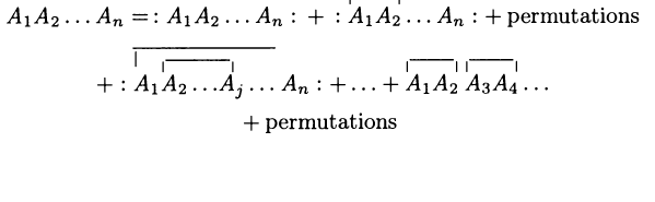Moyal product for Wightman propagator $\Delta_H$ $\begin{aligned} & A_1 \star_H A_2 = \\ & ((-)\cdot (-)) \circ \exp \left( \hbar \int (\Delta_H)^{ab}(x,y) \frac{\delta}{\delta \mathbf{\Phi}^a(x)} \otimes \frac{\delta}{\delta \mathbf{\Phi}^b(y)} \right)(A_1 \otimes A_2) \end{aligned}$
	perturbative expansion of 3) via 1)	Feynman diagrams	Moyal product for Feynman propagator $\Delta_F$ $\begin{aligned} & A_1 \star_F A_2 = \\ & ((-)\cdot (-)) \circ \exp \left( \hbar \int (\Delta_F)^{ab}(x,y) \frac{\delta}{\delta \mathbf{\Phi}^a(x)} \otimes \frac{\delta}{\delta \mathbf{\Phi}^b(y)} \right)(A_1 \otimes A_2) \end{aligned}$

References

See also the references at S-matrix

The equivalence of the time-ordered product on regular observables to the point-wise product was maybe first highlighted in

• Romeo Brunetti, Michael Dütsch, Klaus Fredenhagen, p. 6 of Perturbative Algebraic Quantum Field Theory and the Renormalization Groups, Adv. Theor. Math. Physics 13 (2009), 1541-1599 (arXiv:0901.2038)

and then further amplified in

• Klaus Fredenhagen, Kasia Rejzner, p. 6 of Batalin-Vilkovisky formalism in perturbative algebraic quantum field theory, Commun. Math. Phys. 317(3), 697–725 (2012) (arXiv:1110.5232)