Contents
Context
Functional analysis
Overview diagrams
Basic concepts
Theorems
Topics in Functional Analysis
Riemannian geometry
Vacua
Contents
Idea
In perturbative quantum field theory on curved spacetimes, Hadamard states are certain quantum states of free fields (whose 2-point function is the corresponding Hadamard distribution on spacetime) that play the role that the vacuum state plays on Minkowski spacetime.
Here a vacuum state is supposed to be a quantum state that expresses the absence of any particle excitations of the fields. On Minkowski spacetime the vacuum state for a free field theory is the standard Hadamard state (def. below). On general globally hyperbolic spacetimes there are always Hadamard states (Radzikowski 96, see def. below), and they do play the role of the vacuum state in the construction of AQFT on curved spacetimes, see at locally covariant perturbative AQFT. Notably the choice of such a Hadamard state fixes the Feynman propagator, hence the time-ordered product of quantum observables and thus the perturbative S-matrix away from coinciding interaction points (the extension of these distributions to coinciding interaction points is the process of renormalization).
However, since on a general globally hyperbolic spacetime there is no globally well-defined concept of particles, there is in general no concept of vacuum state. But under good conditions (such as existence of suitable timelike Killing vectors) one may identify Hadamard states which deserve to be thought of as vacuum states (Brum-Fredenhagen 13).
Hadamard states are mathematically characterized as follows:
Given a globally hyperbolic spacetime, the causal propagator defines a symplectic form on the covariant phase space of the free scalar field. However its wave front set is too large for the would-be induced Moyal star product to exist on but a very small subalgebra of smooth functionals, due to the failure of the relevant products of distributions to exist. However the Moyal star product makes sense more generally for almost Kähler structures with a symmetric contribution added to the skew-symmetric symplectic form.
A Hadamard distribution is such a modification of the causal propagator by a symmetric component such that the resulting wave front set is just one causal half of that of the causal propagator. This is usually called a Wightman propagator. (Unfortunately the term “Hadamard propagator” is used for something else.)
This allows to define the corresponding Moyal star product on the larger algebra of microcausal functionals which is large enough to contain the adiabatically switched point interaction terms (as in phi^4 theory etc.). The resulting algebra of observables is the Wick algebra of the free scalar field.
The Hadamard distribution may also be thought of as the 2-point function of a quasi-free quantum state. These states are therefore called Hadamard states.
propagators (i.e. integral kernels of Green functions)
for the wave operator and Klein-Gordon operator
on a globally hyperbolic spacetime such as Minkowski spacetime:
| name | symbol | wave front set | as vacuum exp. value
of field operators | as a product of
field operators |
|---|
| causal propagator | | 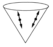
 | | Peierls-Poisson bracket |
| advanced propagator | | | | future part of
Peierls-Poisson bracket |
| retarded propagator | | | | past part of
Peierls-Poisson bracket |
| Wightman propagator | | 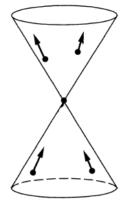 | | positive frequency of
Peierls-Poisson bracket,
Wick algebra-product,
2-point function
of vacuum state
or generally of
Hadamard state |
| Feynman propagator | | 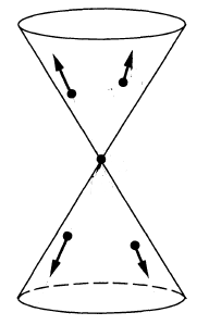 | | time-ordered product |
(see also Kocic‘s overview: pdf)
Definition
Recall the following general facts about the wave equation/Klein-Gordon equation
Proposition
(the causal propagator)
Let be a time-oriented globally hyperbolic spacetime and let (the “mass”). Then the Klein-Gordon equation
(a partial differential equation on smooth functions ) has unique advanced and retarded Green functions , namely continuous linear functionals
(from bump functions to general smooth functions) which are fundamental solutions in that
and which have advanced/retarded support of a distribution when viewed (via the Schwartz kernel theorem) as distributions on the Cartesian product manifold
In fact these two fundamental solutions are related by switching their arguments
Finally their wave front set is
Here the relation means that there exists a lightlike geodesic from to with cotangent vector at and at .
It follows that the wave front set of their difference (the causal propagator)
is
Definition
(Hadamard distribution)
Let be a time oriented globally hyperbolic spacetime.
A Hadamard 2-point function or Hadamard distribution for the free scalar field on is a distribution of two variables
on the Cartesian product manifold such that
-
the anti-symmetric part of is the causal propagator (from prop. )
-
(wave front set spectral condition (Radzikowski 96, def. 6.1))
the wave front set is one causal half that of the causal propagator:
-
(Klein-Gordon bi-solution) and , for all ;
-
(positive semi-definiteness) For any complex-valued bump function we have that
Properties
Existence
(Radzikowski 96, above theorem 6.3 with theorem 5.1)
In fact there exist infinitely many Hadamard distributions on any globally hyperbolic spacetime (Junker-Schrohe 02, Fulling-Narcowich-Wald 81).
Examples
For Klein-Gordon operator on Minkowski spacetime
On Minkowski spacetime consider the Klein-Gordon operator
Its Fourier transform is
The dispersion relation of this equation we write
(1)
where on the right we choose the non-negative square root.
We now discuss
-
Advanced and regarded propagators
-
Causal propagator
-
Wightman propagator
-
Wave front sets
advanced and retarded propagators for Klein-Gordon equation on Minkowski spacetime
Proposition
(mode expansion of advanced and retarded propagators for Klein-Gordon operator on Minkowski spacetime)
The advanced and retarded Green functions of the Klein-Gordon operator on Minkowski spacetime are given by integral kernels (“propagators”)
by (in generalized function-notation)
where the advanced and retarded propagators have the following equivalent expressions:
Here denotes the dispersion relation (1) of the Klein-Gordon equation.
Proof
The Klein-Gordon operator is a Green hyperbolic differential operator (this example) therefore its advanced and retarded Green functions exist uniquely (prop. ). Moreover, prop. says that they are continuous linear functionals with respect to the topological vector space structures on spaces of smooth sections (def. ). In the case of the Klein-Gordon operator this just means that
are continuous linear functionals in the standard sense of distributions. Therefore the Schwartz kernel theorem implies the existence of integral kernels being distributions in two variables
such that, in the notation of generalized functions,
These integral kernels are the advanced/retarded “propagators”. We now compute these integral kernels by making an Ansatz and showing that it has the defining properties, which identifies them by the uniqueness statement of prop. .
We make use of the fact that the Klein-Gordon equation is invariant under the defnining action of the Poincaré group on Minkowski spacetime, which is a semidirect product group of the translation group and the Lorentz group.
Since the Klein-Gordon operator is invariant, in particular, under translations in it is clear that the propagators, as a distribution in two variables, depend only on the difference of its two arguments
Since moreover the Klein-Gordon operator is formally self-adjoint (this prop.) this implies that for the Klein the equation (?)
is equivalent to the equation (?)
Therefore it is sufficient to solve for the first of these two equation, subject to the defining support conditions. In terms of the propagator integral kernels this means that we have to solve the distributional equation
(3)
subject to the condition that the distributional support is
We make the Ansatz that we assume that , as a distribution in a single variable , is a tempered distribution
hence amenable to Fourier transform of distributions. If we do find a solution this way, it is guaranteed to be the unique solution by prop. .
By this prop. the distributional Fourier transform of equation (3) is
(4)
where in the second line we used the Fourier transform of the delta distribution from this example.
Notice that this implies that the Fourier transform of the causal propagator
satisfies the homogeneous equation:
(5)
Hence we are now reduced to finding solutions to (4) such that their Fourier inverse has the required support properties.
We discuss this by a variant of the Cauchy principal value:
Suppose the following limit of non-singular distributions in the variable exists in the space of distributions
meaning that for each bump function the limit in
exists. Then this limit is clearly a solution to the distributional equation (4) because on those bump functions which happen to be products with we clearly have
Moreover, if the limiting distribution (6) exists, then it is clearly a tempered distribution, hence we may apply Fourier inversion to obtain Green functions
To see that this is the correct answer, we need to check the defining support property.
Finally, by the Fourier inversion theorem, to show that the limit (6) indeed exists it is sufficient to show that the limit in (7) exists.
We compute as follows
(8)
where denotes the dispersion relation (1) of the Klein-Gordon equation.
Here the key step is the application of Cauchy's integral formula in the fourth step. We spell this out now for , the discussion for is the same, just with the appropriate signs reversed.
- If thn the expression decays with positive imaginary part of , so that we may expand the integration domain into the upper half plane as
Conversely, if then we may analogously expand into the lower half plane.
- This integration domain may then further be completed to two contour integrations. For the expansion into the upper half plane these encircle counter-clockwise the poles at , while for expansion into the lower half plane no poles are being encircled.
-
Apply Cauchy's integral formula to find in the case the sum of the residues at these two poles times , zero in the other case. (For the retarded propagator we get times the residues, because now the contours encircling non-trivial poles go clockwise).
-
The result does not depend on anymore, therefore the limit is now computed trivially.
This computation shows a) that the limiting distribution indeed exists, and b) that the support of is in the future, and that of is in the past.
Hence it only remains to see now that the support of is inside the causal cone. But this follows from the previous argument, by using that the Klein-Gordon equation is invariant under Lorentz transformations: This implies that the support is in fact in the future of every spacelike slice through the origin in , hence in the closed future cone of the origin.
Corollary
(causal propagator is skew-symmetric)
Under reversal of arguments the advanced and retarded causal propagators are related by
It follows that the causal propagator is skew-symmetric in its arguments:
Proof
By prop. we have with (2)
Here in the second step we applied change of integration variables (which introduces no sign because in addition to the integration domain reverses orientation).
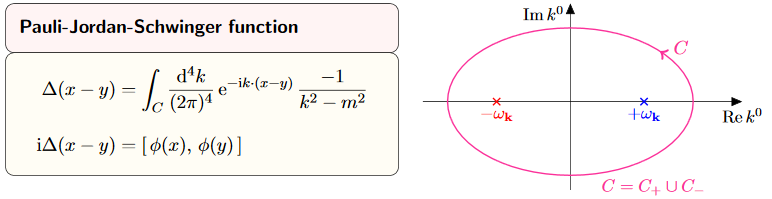
causal propagator
Proposition
(mode expansion of causal propagator for Klein-Gordon equation on Minkowski spacetime)
The causal propagator (?) for the Klein-Gordon equation for mass on Minkowski spacetime is given, in generalized function notation, by
(9)
where in the second line we used Euler's formula .
In particular this shows that the causal propagator is real, in that it is equal to its complex conjugate
(10)
Proof
By definition and using the expression from prop. for the advanced and retarded causal propagators we have
For the reality, notice from the last line that
where in the last step we used the change of integration variables (whih introduces no sign, since on top of the orientation of the integration domain changes).
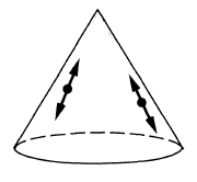
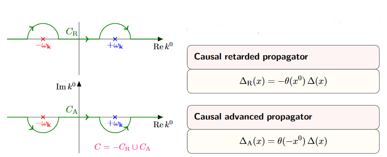
We consider a couple of equivalent expressions for the causal propagator:
graphics grabbed from Kocic 16
Proof
By Cauchy's integral formula we compute as follows:
The last line is the expression for the causal propagator from prop.
Proof
By decomposing the integral over into its negative and its positive half, and applying the change of integration variables we get
The last line is the expression for the causal propagator from prop. .
(e.g. Scharf 95 (2.3.18))
Proof
Consider the formula for the causal propagator in terms of the mode expansion (9). Since the integrand here depends on the wave vector only via its norm and the angle it makes with the given spacetime vector via
we may express the integration in terms of polar coordinates as follws:
We specialize further computation now to the case that the spacetime dimension is , in which case the above becomes
where in the last step we used one of the trigonometric identities.
In order to further evaluate this, we parameterize the remaining components of the wave vector by the dual rapidity , via
as
which makes use of the fact that is non-negative, by construction. This change of integration variables makes the integrals under the braces above become
Next we similarly parameterize the vector by its rapidity . That parameterization depends on whether is spacelike or not, and if not, whether it is future or past directed.
First, if is spacelike in that then we may parameterize as
which yields
where in the last line we observe that the integrand is a skew-symmetric function of .
Second, if is timelike with then we may parameterize as
which yields
Here denotes the Bessel function of order 0. The important point here is that this is a smooth function.
Similarly, if is timelike with then the same argument yields
In conclusion, the general form of is
Therefore we end up with
Wightman propagator
Prop. exhibits the causal propagator of the Klein-Gordon operator on Minkowski spacetime as the difference of a contribution for positive temporal angular frequency (hence positive energy and a contribution of negative temporal angular frequency.
The positive frequency contribution to the causal propagator is called the Wightman propagator (def. below), also known as the the vacuum state 2-point function of the free real scalar field on Minkowski spacetime. Notice that the temporal component of the wave vector is proportional to the negative angular frequency
(see at plane wave), therefore the appearance of the step function in (11) below:
Definition
(Wightman propagator or vacuum state 2-point function for Klein-Gordon operator on Minkowski spacetime)
The Wightman propagator for the Klein-Gordon operator at mass on Minkowski spacetime is the tempered distribution in two variables which as a generalized function is given by the expression
(11)
Here in the first line we have in the integrand the delta distribution of the Fourier transform of the Klein-Gordon operator times a plane wave and times the step function of the temporal component of the wave vector. In the second line we used the change of integration variables , then the definition of the delta distribution and the fact that is by definition the non-negative solution to the Klein-Gordon dispersion relation.
(e.g. Khavkine-Moretti 14, equation (38) and section 3.4)
It is immediate but important that:
Proof
By definition the Wightman propagator is the Fourier transform of distributions of the product of distributions
where in turn the argument of the delta distribution is just times the Fourier transform of the [Klein-Gordon operator]] itsel. This is clearly a solution to the equation
Under Fourier inversion, this is the equation , as in the proof of prop. .
Proposition
(contour integral representation of the Wightman propagator for the Klein-Gordon operator on Minkowski spacetime)
The Wightman propagator from def. is equivalently given by the contour integral
(12)
where the Jordan curve runs counter-clockwise, enclosing the point , but not enclosing the point .
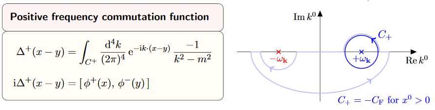
graphics grabbed from Kocic 16
Proof
We compute as follows:
The last step is application of Cauchy's integral formula, which says that the contour integral picks up the residue of the pole of the integrand at . The last line is , by definition .
Proposition
(skew-symmetric part of Wightman propagator is the causal propagator)
The Wightman propagator for the Klein-Gordon equation on Minkowski spacetime (def. ) is of the form
(13)
where
-
is the causal propagator (prop. ), which is real (10) and skew-symmetric (prop. )
-
is real and symmetric
Proof
By applying Euler's formula to (11) we obtain
(14)
On the left this identifies the causal propagator by (9), prop. .
The second summand changes, both under complex conjugation as well as under , via change of integration variables (because the cosine is an even function). This does not change the integral, and hence is symmetric.
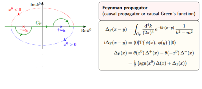
Feynman propagator
We have seen that the positive frequency component of the causal propagator for the Klein-Gordon equation on Minkowski spacetime (prop. ) is the Wightman propagator (def. ) given, according to prop. , by (13)
There is an evident variant of this combination, which will be of interest:
Proposition
(mode expansion for Feynman propagator of Klein-Gordon equation on Minkowski spacetime)
The Feynman propagator (def. ) for the Klein-Gordon equation on Minkowski spacetime is given by the following equivalent expressions
Similarly the anti-Feynman propagator is equivalently given by
Proof
By the mode expansion of from (2) and the mode expansion of from (14) we have
where in the second line we used Euler's formula. The last line follows by comparison with (11) and using that the integral over is invariant under .
The computation for is the same, only now with a minus sign in front of the cosine:
As before for the causal propagator, there are equivalent reformulations of the Feynman propagator, which are useful for computations:
Proof
We compute as follows:
Here
-
In the first step we introduced the complex square root . For this to be compatible with the choice of non-negative square root for in (1) we need to choose that complex square root whose complex phase is one half that of (instead of that plus π). This means that is in the lower half plane and is in the upper half plane.
-
In the third step we observe that
-
for the integrand decays for positive imaginary part and hence the integration over may be deformed to a contour which encircles the pole in the upper half plane;
-
for the integrand decays for negative imaginary part and hence the integration over may be deformed to a contour which encircles the pole in the lower half plane
and then apply Cauchy's integral formula which picks out times the residue a these poles.
Notice that when completing to a contour in the lower half plane we pick up a minus signs from the fact that now the contour runs clockwise.
-
In the fourth step we used prop. .
singular support and wave front sets
We now discuss the singular support and the wave front sets of the various propagators for the Klein-Gordon equation on Minkowski spacetime.
Proof
The statement follows immediately from the result (Gel’fand-Shilov 66, III 2.11 (7), p 294), see this prop.
We make this fully explicit now in the special case of spacetime dimension
by computing an explicit form for the causal propagator in terms of the delta distribution, the Heaviside distribution and smooth Bessel functions.
We follow (Scharf 95 (2.3.18)).
Consider the formula for the causal propagator in terms of the mode expansion (9). Since the integrand here depends on the wave vector only via its norm and the angle it makes with the given spacetime vector via
we may express the integration in terms of polar coordinates as follws:
In the special case of spacetime dimension this becomes
(15)
Here in the second but last step we renamed and doubled the integration domain for convenience, and in the last step we used the trigonometric identity .
In order to further evaluate this, we parameterize the remaining components of the wave vector by the dual rapidity , via
as
which makes use of the fact that is non-negative, by construction. This change of integration variables makes the integrals under the braces above become
(16)
Next we similarly parameterize the vector by its rapidity . That parameterization depends on whether is spacelike or not, and if not, whether it is future or past directed.
First, if is spacelike in that then we may parameterize as
which yields
where in the last line we observe that the integrand is a skew-symmetric function of .
Second, if is timelike with then we may parameterize as
which yields
(17)
Here in the last line we identified the integral representation of the Bessel function of order 0 (see here). The important point here is that this is a smooth function.
Similarly, if is timelike with then the same argument yields
In conclusion, the general form of is
Therefore we end up with
(18)
Proof
The statement follows immediately from the result (Gel’fand-Shilov 66, III 2.11 (7), p 294), see this prop..
We make this fully explicit now in the special case of spacetime dimension
by computing an explicit form for the causal propagator in terms of the delta distribution, the Heaviside distribution and smooth Bessel functions.
We follow (Scharf 95 (2.3.36)).
By (14) we have
The first summand, proportional to the causal propagator, which we computed as (18) in prop. to be
The second term is computed in a directly analogous fashion: The integrals from (16) are now
Parameterizing by rapidity, as in the proof of prop. , one finds that for timelike this is
while for spacelike it is
where we identified the integral representations of the Neumann function (see here) and of the modified Bessel function (see here).
As for the Bessel function in (17) the key point is that these are smooth functions. Hence we conclude that
This expression has singularities on the light cone due to the step functions. In fact the expression being differentiated is continuous at the light cone (Scharf 95 (2.3.34)), so that the singularity on the light cone is not a delta distribution singularity from the derivative of the step functions. Accordingly it does not cancel the singularity of as above, and hence the singular support of is still the whole light cone.
Proposition
(wave front sets of propagators of Klein-Gordon equation on Minkowski spacetime)
The wave front set of the various propagators for the Klein-Gordon equation on Minkowski spacetime, regarded, via translation invariance, as distributions in a single variable, are as follows:
- the causal propagator (prop. ) has wave front set all pairs with and both on the lightcone:
-
- the Wightman propagator (def. ) has wave front set all pairs with and both on the light cone and :
- the Feynman propagator (def. ) has wave front set all pairs with and both on the light cone and
(Radzikowski 96, (16))
Proof
First regarding the causal propagator:
By prop. the singular support of is the light cone.
Since the causal propagator is a solution to the homogeneous Klein-Gordon equation, the propagation of singularities theorem says that also all wave vectors in the wave front set are lightlike. Hence it just remains to show that all non-vanishing lightlike wave vectors based on the lightcone in spacetime indeed do appear in the wave front set.
To that end, let be a bump function whose compact support includes the origin.
For a point on the light cone, we need to determine the decay property of the Fourier transform of . This is the convolution of distributions of with . By prop. we have
This means that the convolution product is the smearing of the mass shell by .
Since the mass shell asymptotes to the light cone, and since for on the light cone (given that is on the light cone), this implies the claim.
Now for the Wightman propagator:
By def. its Fourier transform is of the form
Moreover, its singular support is also the light cone (prop. ).
Therefore now same argument as before says that the wave front set consists of wave vectors on the light cone, but now due to the step function factor it must satisfy .
Finally regarding the Feynman propagator:
by prop. the Feynman propagator coincides with the positive frequency Wightman propagator for and with the “negative frequency Hadamard operator” for . Therefore the form of now follows directly with that of above.
For Dirac operator on Minkowski spacetime
Finally we observe that the propagators for the Dirac field on Minkowski spacetime follow immediately from the propagators for the scalar field:
Proposition
(advanced and retarded propagator for Dirac equation on Minkowski spacetime)
Consider the Dirac operator on Minkowski spacetime, which in Feynman slash notation reads
Its advanced and retarded propagators (def. ) are the derivatives of distributions of the advanced and retarded propagators for the Klein-Gordon equation (prop. ) by :
Hence the same is true for the causal propagator:
Proof
Applying a differential operator does not change the support of a smooth function, hence also not the support of a distribution. Therefore the uniqueness of the advanced and retarded propagators (prop. ) together with the translation-invariance and the anti-formally self-adjointness of the Dirac operator (as for the Klein-Gordon operator (?) implies that it is sufficent to check that applying the Dirac operator to the yields the delta distribution. This follows since the Dirac operator squares to the Klein-Gordon operator:
Similarly we obtain the other propagators for the Dirac field from those of the real scalar field:
Definition
(Wightman propagator for Dirac operator on Minkowski spacetime)
The Wightman propagator for the Dirac operator on Minkowski spacetime is the positive frequency part of the causal propagator (prop. ), hence the derivative of distributions of the Wightman propagator for the Klein-Gordon field (def. ) by the Dirac operator:
Here we used the expression (?) for the Wightman propagator of the Klein-Gordon equation.
Definition
(Feynman propagator for Dirac operator on Minkowski spacetime)
The Feynman propagator for the Dirac operator on Minkowski spacetime is the linear combination
of the Wightman propagator (def. ) and the retarded propagator (prop. ). By prop. this means that it is the derivative of distributions of the Feynman propagator of the Klein-Gordon equation (def. ) by the Dirac operator
References
Textbook discussion of the Hadamard distribution for free fields in Minkowski spacetime is in
(there the Hadamard distribution is denoted “”).
A concise overview of the standard Wightman propagator on Minkowski spacetime and its relation to the other pertinent propagors is given in
- Mikica Kocic, Invariant Commutation and Propagation Functions Invariant Commutation and Propagation Functions, 2016 (pdf)
On general globally hyperbolic spacetimes Hadamard spectrum condition was first rigorously defined in
- B. S. Kay, Robert Wald, Theorems on the uniqueness and thermal properties of stationary, nonsingular, quasifree states on spacetimes with a bifurcate Killing horizon, Phys. Rep. 207(2), 49-136 (1991)
and shown to be equivalent to the definition in terms of singular structure in
- Marek Radzikowski, Micro-local approach to the Hadamard condition in quantum field theory on curved space-time, Commun. Math. Phys. 179 (1996), 529–553 (Euclid)
A gap in the Kay-Wald definition of Hadamard states and in the equivalence with Radzikowski’s formulation has been discussed, by partially changing original Kay-Wald’s definition, and closed in
- Valter Moretti, On the global Hadamard parametrix in QFT and the signed squared geodesic distance defined in domains larger than convex normal neighbourhoods, Lett. Math. Phys. 2021 (arXiv:2107.04903)
Hadamard states with smooth dependence on the mass square (needed for dimensional regularization methods in causal perturbation theory/perturbative AQFT) are constructed in
- Kai Keller, chapter III of Dimensional Regularization in Position Space and a Forest Formula for Regularized Epstein-Glaser Renormalization, PhD thesis (arXxiv:1006.2148)
Discussion of vacuum state-like Hadamard states is in
Review and further developments are in
Discussion for electromagnetism is in
- Claudio Dappiaggi, D. Siemssen, Hadamard states for the vector potential on asymptotically flat spacetimes, Rev. Math. Phys. 25, 1 (2013)
See also
-
W. Junker and E. Schrohe: Adiabatic vacuum states on general spacetime manifolds: Definition, construction, and physical properties, Annales Poincare Phys. Theor. 3, 1113 (2002)
-
S. A. Fulling, M. Sweeny, Robert Wald, Singularity Structure Of The Two Point Function In Quantum Field Theory In Curved Space-Time, Commun. Math. Phys. 63, 257 (1978).
-
S. A. Fulling, F. J. Narcowich, Robert Wald, Singularity Structure Of The Two Point Function In Quantum Field Theory In Curved Space-Time, Annals Phys. 136, 243 (1981),
-
Marcos Brum, Klaus Fredenhagen, “Vacuum-like” Hadamard states for quantum fields on curved spacetimes, Classical and Quantum Gravity, Volume 31, Number 2 (arXiv:1307.0482)