nLab S-matrix
Context
Algebraic Quantum Field Theory
algebraic quantum field theory (perturbative, on curved spacetimes, homotopical)
Concepts
quantum mechanical system, quantum probability
interacting field quantization
Theorems
States and observables
Operator algebra
Local QFT
Perturbative QFT
Functorial Quantum Field Theory
Contents
- Idea
- Details
- In quantum mechanics
- In perturbative relativistic Lagrangian QFT – Causal perturbation theory
- Free field vacua
- Perturbative S-Matrices
- Conceptual remarks
- Interacting field observables
- Time-ordered products
- (“Re”-)Normalization
- Feynman perturbation series
- Effective action
- Vacuum diagrams
- Interacting quantum BV-Differential
- Ward identities
- Retarded products
- In functorial quantum field theory
- Properties
- Examples
- History
- Related entries
- References
Idea
In quantum field theory a scattering amplitude or scattering matrix, usually just S-matrix for short, encodes the probability amplitudes for scattering processes of particles off each other.
General idea
Every Lagrangian perturbative quantum field theory has an S-matrix associated with it (after renormalization), usually thought of as a perturbation series over Feynman diagrams extracted from the Lagrangian density. The rigorous construction of this as an operator-valued distribution is the content of causal perturbation theory (Epstein-Glaser 73).
But there are also S-matrices not fundamentally arising from a local field theory, notably the string scattering amplitudes.
There have been attempts to define perturbative quantum field theory by directly axiomatizing properties of the S-matrix, without requiring concepts of fields in spacetime. This perspective goes back to (Heisenberg 43) and was vocally promoted in Geoffrey Chew‘s “bootstrap program” (a textbook account is in Eden-Ladshoff-Olive-Polkinhorne 66).
In the field theory-picture the crucial condition on the S-matrix is its causal additivity (def. below) which reflects the microcausality of quantum observables (prop. below), whence the name “causal perturbation theory”.
This causality of the S-matrix, when understood in terms of underlying spacetime and fields, is supposed to be detected more abstractly by the S-matrix being a suitable analytic function of the wave vectors of the scattering asymptotic states (Newton 82, 10.3.3, Arkani-Hamed et al. 06), often referred to via “dispersion relations” (e.g. Eden-Ladshoff-Olive-Polkinhorne 66 (1.1.1)-(1.1.5), Gribov 69, 1.1.2). Since thereby analyticity is recognized as the crucial property of the S-matrix in the spacetime/field-independent axiomatization, this is often referred to as “the analytic S-matrix” (e.g. Eden-Ladshoff-Olive-Polkinhorne 66). More specifically microcausality is what induces “crossing symmetry” of the S-matrix (Weinberg 95, section 10.8).
The perception of the nature of the S-matrix as a primary or derived concept in the foundations of quantum field theory has a convoluted (and ongoing) history, see below.
The S-matrix bootstrap
From this Physics.SE comment by Ron Maimon:
The idea of the S-matrix “bootstrap” is that one may compute the S-matrix directly from suitable axioms without using a local quantum field theory involving fields on spacetime. In order for the theory to be interesting, the S-matrix should obey certain properties abstracted away from field theory
- It should be unitary
- It should be Lorentz invariant
- It should be crossing invariant: this means that the antiparticle scattering should be described by the analytic continuation of the particle scattering
- It should obey the Landau property— that all singularities of scattering are poles and cuts corresponding to exchange of collections of real particles on shell.
- It should obey (Mandelstam) analyticity: the amplitude should be writable as an integral over the imaginary part of the cut discontinuity from production of physical particles. Further, this cut discontinuity itself can be expanded in terms of another cut discontinuity (these are the mysterious then and still mysterious now double dispersion relations of Mandelstam).
This is a sketchy summary, because each of these conditions is involved. The unitarity condition in particular, is very difficult, because it is so nonlinear. The only practical way to solve it is in a perturbation series which starts with weakly interacting nearly stable particles (described by poles of the S-matrix) which exchange each other (the exchange picture is required by crossing, and the form of the scattering is fixed by the Landau and Mandelstam analyticity, once you know the spectrum).
The “Bootstrap property” is then the following heuristic idea, which is included in the above formal relations:
- The particles and interactions which emerge as the spectrum of the S-matrix from the scattering of states, including their binding together into bound states, should be the same spectrum of particles that come in ias in-states.
This is a heuristic idea, because it is only saying that the S-matrix is consistent, and the formal consistency relations are those above. But the bootstrap was a slogan that implied that all the consistency conditions were not yet discovered, and there might be more.
This idea was very inspirational to many great people in the 1960s, because it was an approach to strong interactions that could accommodate non-field theories of infinitely many particle types of high spin, without postulating constituent particles (like quarks and gluons).
Regge theory
Continuing with this Physics.SE comment by Ron Maimon:
The theory above doesn’t get you anywhere without the following additional stuff. If you don’t do this, you end up starting with a finite number of particles and interactions, and then you end up in effective field theory land. The finite-number-of-particles version of S-matrix theory is a dead end, or at least, it is equivalent to effective field theory, and this was understood in the late 1960s by Weinberg, and others, and this led S-matrix theory to die. This was the road the Chew travelled on, and the end of this road must be very personally painful to him.
But there is another road for S-matrix theory which is much more interesting, so that Chew should not be disheartened. You need to know that the scattering amplitude is analytic in the angular momentum of the exchanged particles, so that the particles lie on Regge trajectories, which give their angular momentum as a function of their mass squared, s.
Where the Regge trajectories hit an integer angular momentum, you see a particle. The trajectory interpolates the particle mass-squared vs. angular momentum graph, and it gives the asymptotic scattering caused by exchanging all these particles together. This scattering can be softer than the exchange of any one of these particles, because exchanging a particle of high spin necessarily has very singular scattering amplitudes at high energy. The Regge trajectory cancels out this growth with an infinite series of higher particles which soften the blowup, and lead to a power-law near-beam scattering at an angle which shrinks to zero as the energy goes to infinity in a way determined by the shape of the trajectory.
So the Regge bootstrap adds the following conditions
- All the particles in the theory lie on Regge trajectories, and the scattering of these particles is by Regge theory.
This condition is the most stringent, because you can’t deform a pure Regge trajectory by adding a single particle— you have to add new trajectories. The following restriction was suggested by experiment
- The Regge trajectories are linear in s
This was suggested by Chew and Frautschi from the resonances known in 1960! The straight lines mostly had two points. The next condition is also ad-hoc and experimental
- The Regge slope is universal (for mesons), it’s the same for all the trajectories.
There are also “pomerons” in this approach which are not mesons, which have a different Regge slopem but ignore this for now.
Finally, there is the following condition, which was experimentally motivated, but has derivations by Mandelstam and others from more theoretical foundations (although this is S-matrix theory, it doesn’t have axioms, so derivation is a loose word).
- The exchange of trajectories is via the s-channel or the t-channel, but not both. It is double counting to exchange the same trajectories in both channels.
These conditions essentially uniquely determine Veneziano’s amplitude and bosonic string theory. Adding Fermion trajectories requires Ramond style supersymmetry, and then the road to string theory is to reinterpret all these conditions in the string picture which emerges.
String theory incorporates and gives concrete form to all the boostrap ideas, so much so that anyone doing bootstrap today is doing string theory, especially since AdS/CFT showed why the bootstrap is relevant to gauge theories like QCD in the first place.
The highlight of Regge theory is the Reggeon calculus, a full diagrammatic formalism, due to Gribov, for calculating the exchange of pomerons in a perturbation framework. This approach inspired a 2d parton picture of QCD which is studied heavily by several people, notably, Gribov, Lipatov, Feynman (as part of his parton program), and more recently Rajeev. Nearly every problem here is open and interesting.
For an example of a reasearch field which (partly) emerged from this, one of the major motivations for taking PT quantum mechanics seriously was the strange non-Hermitian form of the Reggeon field theory Hamiltonian.
Pomerons and Reggeon Field theory
Further from this Phyics.SE comment by Ron Maimon:
The main success of this picture is describing near-beam scattering, or diffractive scattering, at high energies. The idea here is that there is a Regge trajectory which is called the pomeron, which dominates high energy scattering, and which has no quantum numbers. This means that any particle will exchange the pomeron at high energies, so that p-pbar and p-p total cross sections will become equal.
This idea is spectacularly confirmed by mid 90’s measurements of total p-p and p-pbar cross sections, and in a better political climate, this would have won some boostrap theorists a Nobel prize. Instead, it is never mentioned.
The pomeron in string theory becomes the closed string, which includes the graviton, which couples universally to stress energy. The relation between the closed string and the QCD pomeron is the subject of active research, associated with the names of Lipatov, Polchinski, Tan, and collaborators.
Regge scattering also predicts near beam scattering amplitudes from the sum of the appropriate trajectory function you can exchange. These predictions have been known to roughly work since the late 1960s.
Details
We first discuss the simple situation of S-matrices in quantum mechanics:
Then we give a detailed account of S-matrix theory for perturbative quantum field theory induced from interaction action functionals on spacetime:
This is essentially chapter 15. in A first idea of quantum field theory.
(We should eventually also discuss the abstract S-matrix bootstrap here in detail.)
In quantum mechanics
In quantum mechanics, let be some Hilbert space and let
be an Hermitian operator, thought of as a Hamiltonian, decomposed as the sum of a free part (kinetic energy) and an interaction part (potential energy).
For example for a non-relativistic particle of mass propagating on the line subject to a potential energy , then is the Hilbert space of square integrable functions and
where is the operator of multiplying square integrable functions with the given potential energy function.
Now for
a one-parameter family of quantum states, the Schrödinger equation for this state reads
It is easy to solve this differential equation formally via its Green function: for any state, then the unique solution to the Schrödinger equation subject to is
(One says that this is the solution “in the Schrödinger picture”, whence the subscript.)
However, if is sufficiently complicated, it may still be very hard to extract from this expression a more explicit formula for , such as, in the example of the free particle on the line, its expression as a function (“wave function”) of and .
But assume that the analogous expression for alone is well understood, hence that the operator
is sufficiently well understood. The “interaction picture” is a way to decompose the Schrödinger equation such that its dependence on gets separated from its dependence on in a way that admits to treat in perturbation theory.
Namely define analogously
This is called the solution of the Schrödinger equation “in the interaction picture”, whence the subscript. Its definition may be read as the result of propagating the actual solution at time back to time , but using just the free Hamiltonian, hence with “the interaction switched off”.
Notice that if the operator were to commute with (which it does not in all relevant examples) then we would simply have , hence then the solution (1) in the interaction picture would be the result of “propagating” the initial conditions using only the interaction. Now since may not be assumed to commute with , the actual form of is more complicated. But infinitesimally it remains true that is propagated this way, not by the plain operator , though, but by viewed in the Heisenberg picture of the free theory. This is the content of the differential equation (2) below.
But first notice that this will indeed be useful: If an explicit expression for the “state in the interaction picture” (1) is known, then the assumption that also the operator is sufficiently well understood implies that the actual solution
is under control. Hence the question now is how to find given its value at some time . (It is conventional to consider this for , see (4) below.)
Now observe that satisfies the following differential equation (“Schrödinger equation in interaction picture”):
where
is known as the interaction term “viewed in the interaction picture”.
Here is the derivation of (2), where we use the product law for differentiation:
Now in fact is just “viewed in the Heisenberg picture”, but for the free theory. By our running assumption that the free theory is well understood, also is well understood, and hence all that remains now is to find a sufficiently concrete solution to equation (2). This is the heart of working in the interaction picture.
Solutions to equations of the “parallel transport”-type such as (2) are given by time-ordering of Heisenberg picture operators, denoted , applied to the naive exponential solution as above. This is known as the Dyson formula:
Here time-ordering means
Beware the conventional abuse of notation here: Strictly speaking time ordering acts on the tensor algebra spanned by the and has to be followed by taking tensor products to actual products.
In applications to scattering processes one is interest in prescribing the quantum state/wave function far in the past, hence for , and computing its form far in the future, hence for .
The operator that sends such “asymptotic ingoing-states” to “asymptic outgoing states” is hence the limit
This limit (if it exists) is called the scattering matrix or S-matrix, for short.
For example if and are two interactions such that the support in time of is after the support of :
then, assuming the S-matrix for , and exists, the Dyson formula (3) implies the “causal factorization”
Conversely, decomposing any with the step function as
then this causal factorization-relation may be understood as the integral version of the “Schrödinger equation in the interaction picture” (2).
It is this “integral-version of the Schrödinger equation in the interaction picture” (5) that has a fairly evident generalization from quantum mechanics to relativistic perturbative quantum field theory in the form of causal perturbation theory, def. below, see remark below that.
In perturbative relativistic Lagrangian QFT – Causal perturbation theory
In perturbative algebraic quantum field theory the broad structure of the interaction picture in quantum mechanics (above) remains a very good guide, but various technical details have to be generalized with due care:
-
The algebra of operators in the Heisenberg picture of the free theory becomes the Wick algebra of the free field theory (taking into account “normal ordering” of field operators) defined on microcausal functionals built from operator-valued distributions with constraints on their wave front set.
-
The time-ordered products in the Dyson formula have to be refined to causally ordered products and the resulting product at coincident points has to be defined by point-extension of distributions – the freedom in making this choice is the renormalization freedom (“conter-terms”).
-
The sharp interaction cutoff in the Dyson formula that is hidden in the integration over has to be smoothed out by adiabatic switching of the interaction (making the whole S-matrix an operator-valued distribution).
Together these three points are taken care of by the axiomatization of the “adiabatically switched S-matrix” according to causal perturbation theory (def. below)
Free field vacua
In considering perturbative QFT, we are considering perturbation theory in formal deformation parameters around a fixed free Lagrangian quantum field theory in a chosen Hadamard vacuum state.
For convenient referencing we collect all the structure and notation that goes into this in the following definitions:
Definition
(free relativistic Lagrangian quantum field vacuum)
Let
-
be a spacetime (e.g. Minkowski spacetime);
-
a free Lagrangian field theory (this def.), with field bundle ;
-
a gauge parameter bundle for (this def.), with induced BRST-reduced Lagrangian field theory (this example);
-
a gauge fixing (this def.) with graded BV-BRST field bundle (this remark);
-
a Wightman propagator compatible with the causal propagator which corresponds to the Green hyperbolic Euler-Lagrange equations of motion induced by the gauge-fixed Lagrangian density .
Given this, we write
for the corresponding Wick algebra-structure on formal power series in (Planck's constant) of microcausal polynomial observables. This is a star algebra with respect to (coefficient-wise) complex conjugation.
Write
for the induced Hadamard vacuum state (this prop.), hence the state whose distributional 2-point function is the chosen Wightman propagator:
Given any microcausal polynomial observable then its value in this state is called its free vacuum expectation value
Write
for the inclusion of local observables into microcausal polynomial observables (this example), thought of as forming normal-ordered products in the Wick algebra (by this def.).
We denote the Wick algebra-product (the star product induced by the Wightman propagator ) by juxtaposition (this def.)
If an element has an inverse with respect to this product, we denote that by :
Finally, for we write for its spacetime support (this def.). For two subsets of spacetime we write
for the causal ordering-relation and
for spacelike separation.
Remark
For the purposes of constructing or defining the Wick algebra, the conditions on or could be relaxed. Requiring to be an honest Wightman propagator means that it is a distribution satisfying the Hadamard wavefront condition, as well as addition positivity and normalization requirements. Dropping the positivity and some of the normalization requirements, is then only a Hadamard parametrix for the Wightman propagator. The construction of the Wick algebra with respect to still makes sense, but can no longer be interpreted as normal ordering with respect to a fixed vacuum state. In fact, in locally covariant pAQFT, the property for to be the Wightman propagator for a state is in conflict with local covariance. On the other hand, there is no problem with selecting a locally covariant Hadamard parametrix , which allows the construction or definition of the Wick algebra to be locally covariant.
Being concerned with perturbation theory means mathematically that we consider formal power series in deformation parameters (“Planck's constant”) and (“coupling constant”), also in (“source field”), see also remark . The following collects our notational conventions for these matters:
Definition
(formal power series of observables for perturbative QFT)
Let be a relativistic free vacuum according to def. .
Write
for the space of formal power series in three formal variables
-
(“Planck's constant”),
-
(“source field”)
with coefficients in the topological vector spaces of the off-shell polynomial local observables of the free field theory; similarly for the off-shell microcausal polynomial observables:
Similary
denotes the subspace for which no powers of appear, etc.
Accordingly
denotes the vector space of bump functions on spacetime tensored with the vector space spanned by a single copy of . The elements
may be regarded as spacetime-dependent “coupling constants” with compact support, called adiabatically switched couplings.
Similarly then
is the subspace of those formal power series that are at least linear in or (hence those that vanish if one sets ). Hence every element of this space may be written in the form
where the notation is to suggest that we will think of the coefficient of as an (adiabatically switched) interaction action functional.
In particular for
a formal power series in and of local Lagrangian densities, thought of as a local interaction Lagrangian, and if
is an adiabatically switched coupling as before, then the transgression of the product
is such an adiabatically switched interaction
We also consider the space of off-shell microcausal polynomial observables of the free field theory with formal parameters adjoined
which, in its -dependent, is the space of Laurent series in , hence the space exhibiting also negative formal powers of .
Perturbative S-Matrices
We introduce now the axioms for perturbative scattering matrices relative to a fixed relativistic free Lagrangian quantum field vacuum (def. below) according to causal perturbation theory (def. below). Since the first of these axioms requires the S-matrix to be a formal sum of multi-linear continuous functionals, it is convenient to impose axioms on these directly: this is the axiomatics for time-ordered products in def. below. That these latter axioms already imply the former is the statement of prop. below. Its proof requires a close look at the “reverse-time ordered products” for the inverse S-matrix (def. below) and their induced reverse-causal factorization (prop. below).
Definition
(S-matrix axioms – causal perturbation theory)
Let be a relativistic free vacuum according to def. .
Then a perturbative S-matrix scheme for perturbative QFT around this free vacuum is a function
from local observables to microcausal polynomial observables of the free vacuum theory, with formal parameters adjoined as indicated (def. ), such that the following two conditions “perturbation” and “causal additivity (jointly: ”causal perturbation theory“) hold:
-
There exist multi-linear continuous functionals (over ) of the form
(8)for all , such that:
-
The nullary map is constant on the unit of the Wick algebra
-
The unary map is the inclusion of local observables as normal-ordered products (7)
-
The perturbative S-matrix is the exponential series of these maps in that for all
(9)
-
-
For all perturbative local observables we have
(10)
(The inverse of with respect to the Wick algebra-structure is implied to exist by axiom “perturbation”, see remark below.)
Def. is due to (Epstein-Glaser 73 (1)), following (Stückelberg 49-53, Bogoliubov-Shirkov 59). That the domain of an S-matrix scheme is indeed the space of local observables was made explicit (in terms of axioms for the time-ordered products, see def. below), in (Brunetti-Fredenhagen 99, section 3, Dütsch-Fredenhagen 04, appendix E, Hollands-Wald 04, around (20)). Review includes (Rejzner 16, around def. 6.7, Dütsch 18, section 3.3).
Remark
(invertibility of the S-matrix)
The mutliplicative inverse of the perturbative S-matrix in def. with respect to the Wick algebra-product indeed exists, so that the list of axioms is indeed well defined: By the axiom “perturbation” this follows with the usual formula for the multiplicative inverse of formal power series that are non-vanishing in degree 0:
If we write
then
where the sum does exist in , because (by the axiom “perturbation”) has vanishing coefficient in zeroth order in the formal parameters and , so that only a finite sub-sum of the formal infinite sum contributes in each order in and .
This expression for the inverse of S-matrix may usefully be re-organized in terms of “rever-time ordered products” (def. below), see prop. below.
Notice that is instead the inverse with respect to the time-ordered products (8) in that
(Since the time-ordered product is, by definition, symmetric in its arguments, the usual formula for the multiplicative inverse of an exponential series applies).
Remark
(adjoining further deformation parameters)
The definition of S-matrix schemes in def. has immediate variants where arbitrary countable sets and of formal deformation parameters are considered, instead of just a single coupling constant and a single source field . The more such constants are considered, the “more perturbative” the theory becomes and the stronger the implications.
Given a perturbative S-matrix scheme (def. ) it immediately induces a corresponding concept of observables:
Definition
(generating function scheme for interacting field observables)
Let be a relativistic free vacuum according to def. , let be a corresponding S-matrix scheme according to def. .
The corresponding generating function scheme (for interacting field observables, def. below) is the functional
given by
Proposition
(causal additivity in terms of generating functions)
In terms of the generating functions (def. ) the axiom “causal additivity” on the S-matrix scheme (def. ) is equivalent to:
-
(causal additivity in terms of )
For all local observables we have
(13)
(Whence “additivity”.)
Proof
This follows by elementary manipulations:
Multiplying both sides of (10) by yields
This is the first line of (13).
Multiplying both sides of (10) by yields
This is the second line of (13).
Definition
(interacting field observables – Bogoliubov's formula)
Let be a relativistic free vacuum according to def. , let be a corresponding S-matrix scheme according to def. , and let be a local observable regarded as an adiabatically switched interaction-functional.
Then for a local observable of the free field theory, we say that the corresponding local interacting field observable
is the coefficient of in the generating function (12):
This expression is called Bogoliubov's formula, due to (Bogoliubov-Shirkov 59).
One thinks of as the deformation of the local observable as the interaction is turned on; and speaks of an element of the interacting field algebra of observables. Their value (“expectation value”) in the given free Hadamard vacuum state (def. ) is a formal power series in Planck's constant and in the coupling constant , with coefficients in the complex numbers
which express the probability amplitudes that reflect the predictions of the perturbative QFT, which may be compared to experiment.
(Epstein-Glaser 73, around (74); review includes (Dütsch-Fredenhagen 00, around (17), Dütsch 18, around (3.212)).
Remark
(interacting field observables are formal deformation quantization)
The interacting field observables in def. are indeed formal power series in the formal parameter (Planck's constant), as opposed to being more general Laurent series, hence they involve no negative powers of (Dütsch-Fredenhagen 00, prop. 2 (ii), Hawkins-Rejzner 16, cor. 5.2). This is not immediate, since by def. the S-matrix that they are defined from does involve negative powers of .
It follows in particular that the interacting field observables have a classical limit , which is not the case for the S-matrix itself (due to it involving negative powers of ). Indeed the interacting field observables constitute a formal deformation quantization of the covariant phase space of the interacting field theory (prop. below) and are thus the more fundamental concept.
As the name suggests, the S-matrices in def. serve to express scattering amplitudes (example below). But by remark the more fundamental concept is that of the interacting field observables. Their perspective reveals that consistent interpretation of scattering amplitudes requires the following condition on the relation between the vacuum state and the interaction term:
Definition
Let be a relativistic free vacuum according to def. , let be a corresponding S-matrix scheme according to def. , and let be a local observable, regarded as an adiabatically switched interaction action functional.
We say that the given Hadamard vacuum state (this prop.)
is stable with respect to the interaction , if for all elements of the Wick algebra
we have
Example
(time-ordered product of interacting field observables)
Let be a relativistic free vacuum according to def. , let be a corresponding S-matrix scheme according to def. , and let be a local observable regarded as an adiabatically switched interaction-functional.
Consider two local observables
with causally ordered spacetime support
Then causal additivity according to prop. implies that the Wick algebra-product of the corresponding interacting field observables (def. ) is
Here the last line makes sense if one extends the axioms on the S-matrix in prop. from formal power series in to formal power series in (remark ). Hence in this generalization, the generating functions are not just generating functions for interacting field observables themselves, but in fact for time-ordered products of interacting field observables.
An important special case of time-ordered products of interacting field observables as in example is the following special case of scattering amplitudes, which is the example that gives the scattering matrix in def. its name:
Example
(scattering amplitudes as vacuum expectation values of interacting field observables)
Let be a relativistic free vacuum according to def. , let be a corresponding S-matrix scheme according to def. , and let be a local observable regarded as an adiabatically switched interaction-functional, such that the vacuum state is stable with respect to (def. ).
Consider local observables
whose spacetime support satisfies the following causal ordering:
for all and .
Then the vacuum expectation value of the Wick algebra-product of the corresponding interacting field observables (def. ) is
These vacuum expectation values are interpreted, in the adiabatic limit where , as scattering amplitudes (remark below).
Proof
For notational convenience, we spell out the argument for . The general case is directly analogous.
So assuming the causal order
we compute with causal additivity via prop. as follows:
With this the statement follows by the definition of vacuum stability (def. ).
Remark
(computing S-matrices via Feynman perturbation series)
For practical computation of vacuum expectation values of interacting field observables (example ) and hence in particular, via example , of scattering amplitudes, one needs some method for collecting all the contributions to the formal power series in increasing order in and .
Such a method is provided by the Feynman perturbation series (example below) and the effective action (def. ), see example below.
Conceptual remarks
The simple axioms for S-matrices in causal perturbation theory (def. ) and hence for interacting field observables (def. ) have a wealth of implications and consequences. Before discussing these formally below, we here make a few informal remarks meant to put various relevant concepts into perspective:
Remark
(perturbative QFT and asymptotic expansion of probability amplitudes)
Given a perturbative S-matrix scheme (def. ), then by remark the expectation values of interacting field observables (def. ) are formal power series in the formal parameters and (which are interpreted as Planck's constant, and as the coupling constant, respectively):
This means that there is no guarantee that these series converge for any positive value of and/or . In terms of synthetic differential geometry this means that in perturbative QFT the deformation of the classical free field theory by quantum effects (measured by ) and interactions (meaured by ) is so very tiny as to actually be infinitesimal: formal power series may be read as functions on the infinitesimal neighbourhood in a space of Lagrangian field theories at the point , .
In fact, a simple argument (due to Dyson 52) suggests that in realistic field theories these series never converge for any positive value of and/or . Namely convergence for would imply a positive radius of convergence around , which would imply convergence also for and even for imaginary values of , which would however correspond to unstable interactions for which no converging field theory is to be expected. (See Helling, p. 4 for the example of phi^4 theory.)
In physical practice one tries to interpret these non-converging formal power series as asymptotic expansions of actual but hypothetical functions in , which reflect the actual but hypothetical non-perturbative quantum field theory that one imagines is being approximated by perturbative QFT methods. An asymptotic expansion of a function is a power series which may not converge, but which has for every an estimate for how far the sum of the first terms in the series may differ from the function being approximated.
For examples such as quantum electrodynamics and quantum chromodynamics, as in the standard model of particle physics, the truncation of these formal power series scattering amplitudes to the first handful of loop orders in happens to agree with experiment (such as at the LHC collider) to high precision (for QED) or at least decent precision (for QCD), at least away from infrared phenomena (see remark ).
In summary this says that perturbative QFT is an extremely coarse and restrictive approximation to what should be genuine non-perturbative quantum field theory, while at the same time it happens to match certain experimental observations to remarkable degree, albeit only if some ad-hoc truncation of the resulting power series is considered.
This is strong motivation for going beyond perturbative QFT to understand and construct genuine non-perturbative quantum field theory. Unfortunately, this is a wide-open problem, away from toy examples. Not a single interacting field theory in spacetime dimension has been non-perturbatively quantized. Already a single aspect of the non-perturbative quantization of Yang-Mills theory (as in QCD) has famously been advertized as one of the Millennium Problems of our age; and speculation about non-perturbative quantum gravity is the subject of much activity.
Now, as the name indicates, the axioms of causal perturbation theory (def. ) do not address non-perturbative aspects of non-perturbative field theory; the convergence or non-convergence of the formal power series that are axiomatized by Bogoliubov's formula (def. ) is not addressed by the theory. The point of the axioms of causal perturbation theory is to give rigorous mathematical meaning to everything else in perturbative QFT.
Remark
(Dyson series and Schrödinger equation in interaction picture)
The axiom “causal additivity” (10) on an S-matrix scheme (def. ) implies immediately this seemingly weaker condition (which turns out to be equivalent, this is prop. below):
-
For all local observables we have
(This is the special case of “causal additivity” for , using that by the axiom “perturbation” (9) we have .)
If we now think of and themselves as adiabatically switched interaction action functionals, then this becomes
This exhibits the S-matrix-scheme as a “causally ordered exponential” or “Dyson series” of the interaction, hence as a refinement to relativistic field theory of what in quantum mechanics is the “integral version of the Schrödinger equation in the interaction picture” (5). (See also Scharf 95, second half of 0.3).
The relevance of manifest causal additivity of the S-matrix, over just causal factorization (even though both conditions happen to be equivalent, see prop. below), is that it directly implies that the induced interacting field algebra of observables (def. ) forms a causally local net (prop. below).
Remark
(path integral-intuition)
In informal discussion of perturbative QFT going back to informal ideas of Schwinger-Tomonaga-Feynman-Dyson, the perturbative S-matrix is thought of in terms of a would-be path integral, symbolically written
Here the would-be integration is thought to be over the space of field histories (the space of sections of the given field bundle) for field histories which satisfy given asymptotic conditions at ; and as these boundary conditions vary the above is regarded as a would-be integral kernel that defines the required operator in the Wick algebra (e.g. Weinberg 95, around (9.3.10) and (9.4.1)). This is related to the intuitive picture of the Feynman perturbation series expressing a sum over all possible interactions of virtual particles (remark ).
Beyond toy examples, it is not known how to define the would-be measure and it is not known how to make sense of this expression as an actual integral.
The analogous path-integral intuition for Bogoliubov's formula for interacting field observables (def. ) symbolically reads
If here we were to regard the expression
as a would-be Gaussian measure on the space of field histories, normalized to a would-be probability measure, then this formula would express interacting field observables as ordinary expectation values
As before, beyond toy examples it is not known how to make sense of this as an actual integration.
But we may think of the axioms for the S-matrix in causal perturbation theory (def. ) as rigorously defining the path integral, not analytically as an actual integration, but synthetically by axiomatizing the properties of the desired outcome of the would-be integration:
The analogy with a well-defined integral and the usual properties of an exponential vividly suggest that the would-be path integral should obey causal factorization. Instead of trying to make sense of path integration so that this factorization property could then be appealed to as a consequence of general properties of integration and exponentials, the axioms of causal perturbation theory directly prescribe the desired factorization property, without insisting that it derives from an actual integration.
The great success of path integral-intuition in the development of quantum field theory, despite the dearth of actual constructions, indicates that it is not the would-be integration process as such that actually matters in field theory, but only the resulting properties that this suggests the S-matrix should have; which is what causal perturbation theory axiomatizes. Indeed, the simple axioms of causal perturbation theory rigorously imply finite (i.e. ("re"-)normalized) perturbative quantum field theory (see remark ).
Remark
Let be a relativistic free vacuum according to def. , let be a corresponding S-matrix scheme according to def. , and let
be a local observable, regarded as an adiabatically switched interaction action functional.
Then for
two microcausal polynomial observables, with causal ordering
the corresponding scattering amplitude (as in example ) is the value (called “expectation value” when referring to , or “matrix element” when referring to , or “transition amplitude” when referring to and )
for the Wick algebra-product in the given Hadamard vacuum state .
If here and are monomials in Wick algebra-products of the field observables , then this scattering amplitude comes from the integral kernel
or similarly, under Fourier transform of distributions,
These are interpreted as the (distributional) probability amplitudes for plane waves of field species with wave vector to come in from the far past, ineract with each other via , and emerge in the far future as plane waves of field species with wave vectors .
Or rather:
Remark
(adiabatic limit, infrared divergences and interacting vacuum)
Since a local observable by definition has compact spacetime support, the scattering amplitudes in remark describe scattering processes for interactions that vanish (are “adiabatically switched off”) outside a compact subset of spacetime. This constraint is crucial for causal perturbation theory to work.
There are several aspects to this:
-
(adiabatic limit) On the one hand, real physical interactions (say the electron-photon interaction) are not really supposed to vanish outside a compact region of spacetime. In order to reflect this mathematically, one may consider a sequence of adiabatic switchings (each of compact support) whose limit is the constant function (the actual coupling constant), then consider the corresponding sequence of interaction action functionals and finally consider:
-
as the true scattering amplitude the corresponding limit
of adiabatically switched scattering amplitudes (remark ) – if it exists. This is called the strong adiabatic limit.
-
as the true n-point functions the corresponding limit
of tempered distributional expectation values of products of interacting field observables (def. ) – if it exists. (Similarly for time-ordered products.) This is called the weak adiabatic limit.
Beware that the left hand sides here are symbolic: Even if the limit exists in expectation values, in general there is no actual observable whose expectation value is that limit.
The strong and weak adiabatic limits have been shown to exist if all fields are massive (Epstein-Glaser 73). The weak adiabatic limit has been shown to exists for quantum electrodynamics and for mass-less phi^4 theory (Blanchard-Seneor 75) and for larger classes of field theories in (Duch 17, p. 113, 114).
If these limits do not exist, one says that the perturbative QFT has an infrared divergence.
-
-
(algebraic adiabatic limit) On the other hand, it is equally unrealistic that an actual experiment detects phenomena outside a given compact subset of spacetime. Realistic scattering experiments (such as the LHC) do not really prepare or measure plane waves filling all of spacetime as described by the scattering amplitudes (15). Any observable that is realistically measurable must have compact spacetime support. We see below in prop. that such interacting field observables with compact spacetime support may be computed without taking the adiabatic limit: It is sufficient to use any adiabatic switching which is constant on the support of the observable.
This way one obtains for each causally closed subset of spacetime an algebra of observables whose support is in , and for each inclusion of subsets a corresponding inclusion of algebras of observables (prop. below). Of this system of observables one may form the category-theoretic inductive limit to obtain a single global algebra of observables.
This always exists. It is called the algebraic adiabatic limit (going back to Brunetti-Fredenhagen 00, section 8).
For quantum electrodynamics the algebraic adiabatic limit was worked out in (Dütsch-Fredenhagen 98, reviewed in Dütsch 18, 5,3).
-
(interacting vacuum) While, via the above algebraic adiabatic limit, causal perturbation theory yields the correct interacting field algebra of quantum observables independent of choices of adiabatic switching, a theory of quantum probability requires, on top of the algebra of observables, also a state
Just as the interacting field algebra of observables is a deformation of the free field algebra of observables (Wick algebra), there ought to be a corresponding deformation of the free Hadamard vacuum state into an “interacting vacuum state” .
Sometimes the weak adiabatic limit serves to define the interacting vacuum (see Duch 17, p. 113-114).
A stark example of these infrared issues is the phenomenon of confinement of quarks to hadron bound states (notably to protons and neutrons) at large wavelengths. This is paramount in observation and reproduced in numerical lattice gauge theory simulation, but is invisible to perturbative quantum chromodynamics in its free field vacuum state, due to infrared divergences. It is expected that this should be rectified by the proper interacting vacuum of QCD (Rafelski 90, pages 12-16), which is possibly a “theta-vacuum” exhibiting superposition of QCD instantons (Schäfer-Shuryak 98, section III.D). This remains open, closely related to the Millennium Problem of quantization of Yang-Mills theory.
In contrast to the above subtleties about the infrared divergences, any would-be UV-divergences in perturbative QFT are dealt with by causal perturbation theory:
Remark
(the traditional error leading to UV-divergences)
Naively it might seem that (say over Minkowski spacetime, for simplicity) examples of time-ordered products according to def. might simply be obtained by multiplying Wick algebra-products with step functions of the time coordinates, hence to write, in the notation as generalized functions (remark ):
and analogously for time-ordered products of more arguments (for instance Weinberg 95, p. 143, between (3.5.9) and (3.5.10)).
This however is simply a mathematical error (as amplified in Scharf 95, below (3.2.4), below (3.2.44) and in fig. 3):
Both as well as are distributions and their product of distributions is in general not defined (Hörmander's criterion may be violated). The notorious ultraviolet divergences which plagued (Feynman 85) the original conception of perturbative QFT due to Schwinger-Tomonaga-Feynman-Dyson are the signature of this ill-defined product (see remark ).
On the other hand, when both distributions are restricted to the complement of the diagonal (i.e. restricted away from coinciding points ), then the step function becomes a non-singular distribution so that the above expression happens to be well defined and does solve the axioms for time-ordered products.
Hence what needs to be done to properly define the time-ordered product is to choose an extension of distributions of the above product expression back from the complement of the diagonal to the whole space of tuples of points. Any such extension will produce time-ordered products.
There are in general several different such extensions. This freedom of choice is the freedom of "re-"normalization; or equivalently, by the main theorem of perturbative renormalization theory (theorem ), this is the freedom of choosing “counter terms” for the local interactions. This we discuss below in Feynman diagrams and (re-)normalization.
Remark
(absence of ultraviolet divergences and re-normalization)
The simple axioms of causal perturbation theory (def. ) do fully capture perturbative quantum field theory “in the ultraviolet”: A solution to these axioms induces, by definition, well-defined perturbative scattering amplitudes (remark ) and well-defined perturbative probability amplitudes of interacting field observables (def. ) induced by local action functionals (describing point-interactions such as the electron-photon interaction). By the main theorem of perturbative renormalization (theorem ) such solutions exist. This means that, while these are necessarily formal power series in and (remark ), all the coefficients of these formal power series (“loop order contributions”) are well defined.
This is in contrast to the original informal conception of perturbative QFT due to Schwinger-Tomonaga-Feynman-Dyson, which in a first stage produced ill-defined diverging expressions for the coefficients (due to the mathematical error discussed in remark below), which were then “re-normalized” to finite values, by further informal arguments.
Here in causal perturbation theory no divergences in the coefficients of the formal power series are considered in the first place, all coefficients are well-defined, hence “finite”. In this sense causal perturbation theory is about “finite” perturbative QFT, where instead of “re-normalization” of ill-defined expressions one just encounters “normalization” (prominently highlighted in Scharf 95, see title, introduction, and section 4.3), namely compatible choices of these finite values. The actual “re-normalization” in the sense of “change of normalization” is expressed by the Stückelberg-Petermann renormalization group.
This refers to those divergences that are known as UV-divergences, namely short-distance effects, which are mathematically reflected in the fact that the perturbative S-matrix scheme (def. ) is defined on local observables, which, by their very locality, encode point-interactions. See also remark on infrared divergences.
Remark
(virtual particles, worldline formalism and perturbative string theory)
It is suggestive to think of the edges in the Feynman diagrams (def. ) as worldlines of “virtual particles” and of the vertices as the points where they collide and transmute. (Care must be exercised not to confuse this with concepts of real particles.) With this interpretation prop. may be read as saying that the scattering amplitude for given external source fields (remark ) is the superposition of the Feynman amplitudes of all possible ways that these may interact; which is closely related to the intuition for the path integral (remark ).
This intuition is made precise by the worldline formalism of perturbative quantum field theory (Strassler 92). This is the perspective on perturbative QFT which directly relates perturbative QFT to perturbative string theory (Schmidt-Schubert 94). In fact the worldline formalism for perturbative QFT was originally found by taking thre point-particle limit of string scattering amplitudes (Bern-Kosower 91, Bern-Kosower 92).
Remark
Beware the terminology in def. : A single S-matrix is one single observable
for a fixed (adiabatically switched local) interaction , reflecting the scattering amplitudes (remark ) with respect to that particular interaction. Hence the function
axiomatized in def. is really a whole scheme for constructing compatible S-matrices for all possible (adiabatically switched, local) interactions at once.
Since the usual proof of the construction of such schemes of S-matrices involves ("re"-)normalization, the function axiomatized by def. may also be referred to as a ("re"-)normalization scheme.
This perspective on as a renormalization scheme is amplified by the main theorem of perturbative renormalization (theorem ) wich states that the space of choices for is a torsor over the Stückelberg-Petermann renormalization group.
Remark
The axioms for the S-matrix in def. (and similarly that for the time-ordered products below in def. ) are sufficient to imply a causally local net of perturbative interacting field algebras of quantum observables (prop. below), and thus its algebraic adiabatic limit (remark ).
It does not guarantee, however, that the BV-BRST differential passes to those algebras of quantum observables, hence it does not guarantee that the infinitesimal symmetries of the Lagrangian are respected by the quantization process (there may be “quantum anomalies”). The extra condition that does ensure this is the quantum master Ward identity or quantum master equation. This we discuss elsewhere.
Apart from gauge symmetries one also wants to require that rigid symmetries are preserved by the S-matrix, notably Poincare group-symmetry for scattering on Minkowski spacetime. This extra axiom is needed to imply the main theorem of perturbative renormalization (theorem ).
Interacting field observables
We have seen that via Bogoliubov's formula (def. ) every perturbative S-matrix scheme (def. ) induces for every choice of adiabatically switched interaction action functional a notion of perturbative interacting field observables (def. ). These generate an algebra (def. below). By Bogoliubov's formula, in general this algebra depends on the choice of adiabatic switching; which however is not meant to be part of the physics, but just a mathematical device for grasping global field structures locally.
But this spurious dependence goes away (prop. below) when restricting attention to observables whose spacetime support is inside a compact causally closed subsets of spacetime (def. below). This is a sensible condition for an observable in physics, where any realistic experiment nessecarily probes only a compact subset of spacetime, see also remark .
The resulting system (a “co-presheaf”) of well-defined perturbative interacting field algebras of observables (def. below)
is in fact causally local (prop. below). This fact was presupposed without proof already in Il’in-Slavnov 78; because this is one of two key properties that the Haag-Kastler axioms (Haag-Kastler 64) demand of an intrinsically defined quantum field theory (i.e. defined without necessarily making recourse to the geometric backdrop of Lagrangian field theory). The only other key property demanded by the Haag-Kastler axioms is that the algebras of observables be C*-algebras; this however must be regarded as the axiom encoding non-perturbative quantum field theory and hence is necessarily violated in the present context of perturbative QFT.
Since quantum field theory following the full Haag-Kastler axioms is commonly known as AQFT, this perturbative version, with causally local nets of observables but without the C*-algebra-condition on them, has come to be called perturbative AQFT (Dütsch-Fredenhagen 01, Fredenhagen-Rejzner 12).
In this terminology the content of prop. below is that while the input of causal perturbation theory is a gauge fixed Lagrangian field theory, the output is a perturbative algebraic quantum field theory:
The independence of the causally local net of localized interacting field algebras of observables from the choice of adiabatic switching implies a well-defined spacetime-global algebra of observables by forming the inductive limit
This is also called the algebraic adiabatic limit, defining the algebras of observables of perturbative QFT “in the infrared”. The only remaining step in the construction of a perturbative QFT that remains is then to find an interacting vacuum state
on the global interacting field algebra . This is related to the actual adiabatic limit, and it is by and large an open problem, see remark .
Definition
(interacting field algebra of observables – quantum Møller operator)
Let be a relativistic free vacuum according to def. , let be a corresponding S-matrix scheme according to def. , and let be a local observable regarded as an adiabatically switched interaction-functional.
We write
for the subspace of interacting field observables (def. ) corresponding to local observables , the local interacting field observables.
Furthermore we write
for the factorization of the function through its image, which, by remark , is a linear isomorphism with inverse
This may be called the quantum Møller operator (Hawkins-Rejzner 16, (33)).
Finally we write
for the smallest subalgebra of the Wick algebra containing the interacting local observables. This is the perturbative interacting field algebra of observables.
The definition of the interacting field algebra of observables from the data of a scattering matrix (def. ) via Bogoliubov's formula (def. ) is physically well-motivated, but is not immediately recognizable as the result of applying a systematic concept of quantization (such as formal deformation quantization) to the given Lagrangian field theory. The following proposition says that this is nevertheless the case. (The special case of this statement for free field theory is discussed at Wick algebra, see this remark).
Proposition
(interacting field algebra of observables is formal deformation quantization of interacting Lagrangian field theory)
Let be a relativistic free vacuum according to def. , and let be an adiabatically switched interaction Lagrangian density with corresponding action functional .
Then, at least on regular polynomial observables, the construction of perturbative interacting field algebras of observables in def. is a formal deformation quantization of the interacting Lagrangian field theory .
(Hawkins-Rejzner 16, prop. 5.4, Collini 16)
The following definition collects the system (a co-presheaf) of generating functions for interacting field observables which are localized in spacetime as the spacetime localization region varies:
Definition
(system of spacetime-localized generating functions for interacting field observables)
Let be a relativistic free vacuum according to def. , let be a corresponding S-matrix scheme according to def. , and let
be a Lagrangian density, to be thought of as an interaction, so that for an adiabatic switching the transgression
is a local observable, to be thought of as an adiabatically switched interaction action functional.
For a causally closed subset of spacetime (this def.) and for an adiabatic switching function (this def.) which is constant on a neighbourhood of , write
for the smallest subalgebra of the Wick algebra which contains the generating functions (def. ) with respect to for all those local observables whose spacetime support is in .
Moreover, write
be the subalgebra of the Cartesian product of all these algebras as ranges over cutoffs, which is generated by the tuples
for with .
We call the algebra of generating functions for interacting field observables localized in .
Finally, for an inclusion of two causally closed subsets, let
be the algebra homomorphism which is given simply by restricting the index set of tuples.
This construction defines a functor
from the poset of causally closed subsets of spacetime to the category of algebras.
(extends to star algebras if scattering matrices are chosen unitary…)
(Brunetti-Fredenhagen 99, (65)-(67))
The key technical fact is the following:
Proposition
(localized interacting field observables independent of adiabatic switching)
Let be a relativistic free vacuum according to def. , let be a corresponding S-matrix scheme according to def. , and let
be a Lagrangian density, to be thought of as an interaction, so that for an adiabatic switching the transgression
is a local observable, to be thought of as an adiabatically switched interaction action functional.
If two such adiabatic switchings agree on a causally closed subset
in that
then there exists a microcausal polynomial observable
such that for every local observable
with spacetime support in
the corresponding two generating functions (12) are related via conjugation by :
In particular this means that for every choice of adiabatic switching the algebra of generating functions for interacting field observables computed with is canonically isomorphic to the abstract algebra (def. ), by the evident map on generators:
(Brunetti-Fredenhagen 99, prop. 8.1)
Proof
By causal closure of , this lemma says that there are bump functions
which decompose the difference of adiabatic switchings
subject to the causal ordering
With this the result follows from repeated use of causal additivity in its various equivalent incarnations from prop. :
This proves the existence of elements as claimed.
It is clear that conjugation induces an algebra homomorphism, and since the map is a linear isomorphism on the space of generators, it is an algebra isomorphism on the algebras being generated (17).
(While the elements in (16) are far from being unique themselves, equation (16) says that the map on generators induced by conjugation with is independent of this choice.)
Proposition
(system of generating algebras is causally local net)
Let be a relativistic free vacuum according to def. , let be a corresponding S-matrix scheme according to def. , and let
be a Lagrangian density, to be thought of as an interaction.
Then the system
of localized generating functions for interacting field observables (def. ) is a causally local net in that it satisfies the following conditions:
-
(isotony) For every inclusion of causally closed subsets of spacetime the corresponding algebra homomorphism is a monomorphism
-
(causal locality) For two causally closed subsets which are spacelike separated, in that their causal ordering (this def.) satisfies
and for any further causally closed subset which contains both
then the corresponding images of the generating function algebras of interacting field observables localized in and in , respectively, commute with each other as subalgebras of the generating function algebras of interacting field observables localized in :
(Dütsch-Fredenhagen 00, section 3, following Brunetti-Fredenhagen 99, section 8, Il’in-Slavnov 78)
Proof
Isotony is immediate from the definition of the algebra homomorphisms in def. .
By the isomorphism (17) we may check causal localizy with respect to any choice of adiabatic switching constant over . For this the statement follows, with the assumption of spacelike separation, by causal additivity (prop. ):
For and we have:
With the causally local net of localized generating functions for interacting field observables in hand, it is now immediate to get the
Definition
(system of interacting field algebras of observables)
Let be a relativistic free vacuum according to def. , let be a corresponding S-matrix scheme according to def. , and let
be a Lagrangian density, to be thought of as an interaction, so that for an adiabatic switching the transgression
is a local observable, to be thought of as an adiabatically switched interaction action functional.
For a causally closed subset of spacetime (this def.) and for an compatible adiabatic switching function (def. ) write
for the interacting field algebra of observables (def. ) with spacetime support in .
Let then
be the subalgebra of the Cartesian product of all these algebras as ranges, which is generated by the tuples
for .
Finally, for an inclusion of two causally closed subsets, let
be the algebra homomorphism which is given simply by restricting the index set of tuples.
This construction defines a functor
from the poset of causally closed subsets in the spacetime to the category of star algebras.
Finally, as a direct corollary of prop. , we obtain the key result:
Proposition
(system of interacting field algebras of observables is causally local)
Let be a relativistic free vacuum according to def. , let be a corresponding S-matrix scheme according to def. , and let
be a Lagrangian density, to be thought of as an interaction, then the system of algebras of observables (def. ) is a local net of observables in that
-
(isotony) For every inclusion of causally closed subsets the corresponding algebra homomorphism is a monomorphism
-
(causal locality) For two causally closed subsets which are spacelike separated, in that their causal ordering (this def.) satisfies
and for any further causally closed subset which contains both
then the corresponding images of the generating algebras of and , respectively, commute with each other as subalgebras of the generating algebra of :
(Dütsch-Fredenhagen 00, below (17), following Brunetti-Fredenhagen 99, section 8, Il’in-Slavnov 78)
Proof
The first point is again immediate from the definition (def. ).
For the second point it is sufficient to check the commutativity relation on generators. For these the statement follows with prop. :
Time-ordered products
Definition suggests to focus on the multilinear operations which define the perturbative S-matrix order-by-order in . We impose axioms on these time-ordered products directly (def. ) and then prove that these axioms imply the axioms for the corresponding S-matrix (prop. below).
Definition
Let be a free vacuum according to def. .
A time-ordered product is a sequence of multi-linear continuous functionals for all of the form
(from tensor products of local observables to microcausal polynomial observables, with formal parameters adjoined according to def. ) such that the following conditions hold for all possible arguments:
-
(normalization)
-
(perturbation)
-
(symmetry) each is symmetric in its arguments, in that for every permutation of elements
-
(causal factorization) If the spacetime support (this def.) of local observables satisfies the causal ordering
then the time-ordered product of these arguments factors as the Wick algebra-product of the time-ordered product of the first and that of the second arguments:
Example
(S-matrix scheme implies time-ordered products)
Let be a relativistic free vacuum according to def. and let
be a corresponding S-matrix scheme according to def. .
Then the are time-ordered products in the sense of def. .
Proof
We need to show that the satisfy causal factorization.
For
a local observable, consider the continuous linear function that muliplies this by any real number
Since the by definition are continuous linear functionals, they are in particular differentiable maps, and hence so is the S-matrix . We may extract from by differentiation with respect to the parameters at :
for all .
Now the causal additivity of the S-matrix implies its causal factorization (remark ) and this implies the causal factorization of the by the product law of differentiation:
The converse implication, that time-ordered products induce an S-matrix scheme involves more work (prop. below).
Remark
(time-ordered products as generalized functions)
It is convenient (as in Epstein-Glaser 73) to think of time-ordered products (def. ), being Wick algebra-valued distributions (hence operator-valued distributions if we were to choose a representation of the Wick algebra by linear operators on a Hilbert space), as generalized functions depending on spacetime points:
If
is a finite set of horizontal differential forms, and
is a corresponding set of bump functions on spacetime (adiabatic switchings), so that
is the corresponding set of local observables, then we may write the time-ordered product of these observables as the integration of these bump functions against a generalized function with values in the Wick algebra:
Moreover, the subscripts on these generalized functions will always be clear from the context, so that in computations we may notationally suppress these.
Finally, due to the “symmetry” axiom in def. , a time-ordered product depends, up to signs, only on its set of arguments, not on the order of the arguments. We will write and for sets of spacetime points, and hence abbreviate the expression for the “value” of the generalized function in the above as etc.
In this condensed notation the above reads
This condensed notation turns out to be greatly simplify computations, as it absorbs all the “relative” combinatorial prefactors:
Example
(product of perturbation series in generalized function-notation)
Let
and
be power series of Wick algebra-valued distributions in the generalized function-notation of remark .
Then their product with generalized function-representation
is given simply by
Proof
For fixed cardinality the sum over all subsets overcounts the sum over partitions of the coordinates as precisely by the binomial coefficient . Here the factor of cancels against the “global” combinatorial prefactor in the above expansion of , while the remaining factor is just the “relative” combinatorial prefactor seen at total order when expanding the product .
In order to prove that the axioms for time-ordered products do imply those for a perturbative S-matrix (prop. below) we need to consider the corresponding reverse-time ordered products:
Definition
(reverse-time ordered products)
Given a time-ordered product (def. ), its reverse-time ordered product
for is defined by
where the sum is over all unshuffles of into non-empty ordered subsequences. Alternatively, in the generalized function-notation of remark , this reads
Proposition
(reverse-time ordered products express inverse S-matrix)
Given time-ordered products (def. ), then the corresponding reverse time-ordered product (def. ) expresses the inverse (according to remark ) of the corresponding perturbative S-matrix scheme (def. ):
Proof
For brevity we write just “” for . (Hence we assume without restriction that is not independent of powers of and ; this is just for making all sums in the following be order-wise finite sums.)
By definition we have
where all the happen to coincide: .
If instead of unshuffles (i.e. partitions into non-empty subsequences preserving the original order) we took partitions into arbitrarily ordered subsequences, we would be overcounting by the factorial of the length of the subsequences, and hence the above may be equivalently written as:
where denotes the symmetric group (the set of all permutations of elements).
Moreover, since all the are equal, the sum is in fact independent of , it only depends on the length of the subsequences. Since there are permutations of elements the above reduces to
where in the last line we used (11).
In fact prop. is a special case of the following more general statement:
Proposition
(inversion relation for reverse-time ordered products)
Let be time-ordered products according to def. . Then the reverse-time ordered products according to def. satisfies the following inversion relation for all (in the condensed notation of remark ):
and
Proof
This is immediate from unwinding the definitions.
Proposition
(reverse causal factorization of reverse-time ordered products)
Let be time-ordered products according to def. . Then the reverse-time ordered products according to def. satisfies reverse-causal factorization.
(Epstein-Glaser 73, around (15))
Proof
In the condensed notation of remark , we need to show that for with then
We proceed by induction. If the statement is immediate. So assume that the statement is true for sets of cardinality and consider with .
We make free use of the condensed notation as in example .
From the formal inversion
(which uses the induction assumption that ) it follows that
Here
- in the second line we used that , together with the
causal factorization property of (which holds by def. ) and that of
(which holds by the induction assumption, using that hence that ).
-
in the third line we decomposed the sum over into two sums over subsets of and :
-
The first summand in the third line is the contribution where has a non-empty intersection with . This makes range without constraint, and therefore the sum in the middle vanishes, as indicated, as it is the contribution at order of the inversion formula from prop. .
-
The second summand in the third line is the contribution where does not intersect . Now the sum over is the inversion formula from prop. except for one term, and so it equals that term.
-
Using these facts about the reverse-time ordered products, we may finally prove that time-ordered products indeed do induced a perturbative S-matrix:
Proposition
(time-ordered products induce S-matrix)
Let be a system of time-ordered products according to def. . Then
Proof
The axiom “perturbation” of the S-matrix is immediate from the axioms “perturbation” and “normalization” of the time-ordered products. What requires proof is that causal additivity of the S-matrix follows from the causal factorization property of the time-ordered products.
Notice that also the weaker causal factorization property of the S-matrix (remark ) is immediate from the causal factorization condition on the time-ordered products.
But causal additivity is stronger. It is remarkable that this, too, follows from just the time-ordering (Epstein-Glaser 73, around (73)):
To see this, first expand the generating function (12) into powers of and
and then compare order-by-order with the given time-ordered product and its induced reverse-time ordered product (def. ) via prop. . (These are also called the “generating retarded products, discussed in their own right around def. below.)
In the condensed notation of remark and its way of absorbing combinatorial prefactors as in example this yields at order the coefficient
We claim now that the support of is inside the subset for which is in the causal past of . This will imply the claim, because by multi-linearity of it then follows that
and by prop. this is equivalent to causal additivity of the S-matrix.
It remains to prove the claim:
Consider such that the subset of points not in the past of , hence the maximal subset with causal ordering
is non-empty. We need to show that in this case (in the sense of generalized functions).
Write for the complementary set of points, so that all points of are in the past of . Notice that this implies that is also not in the past of :
With this decomposition of , the sum in (18) over subsets of may be decomposed into a sum over subsets of and of , respectively. These subsets inherit the above causal ordering, so that by the causal factorization property of (def. ) and (prop. ) the time-ordered and reverse time-ordered products factor on these arguments:
Here the sub-sum in brackets vanishes by the inversion formula, prop. .
In conclusion:
Proposition
(S-matrix scheme via causal factorization)
Let be a relativistic free vacuum according to def. and consider a function
from local observables to microcausal polynomial observables which satisfies the condition “perturbation” from def. . Then the following two conditions on are equivalent
-
causal additivity (def. )
-
causal factorization (remark )
and hence either of them is necessary and sufficient for to be a perturbative S-matrix scheme according to def. .
Proof
That causal factorization follows from causal additivity is immediate (remark ).
Conversely, causal factorization of implies that its expansion coefficients are time-ordered products (def. ), via the proof of example , and this implies causal additivity by prop. .
(“Re”-)Normalization
We discuss now that time-ordered products as in def. , hence, by prop. , perturbative S-matrix schemes (def. ) exist in fact uniquely away from coinciding interaction points (prop. below).
This means that the construction of full time-ordered products/S-matrix schemes may be phrased as an extension of distributions of time-ordered products to the diagonal locus of coinciding spacetime arguments (prop. below). This choice in their definition is called the choice of ("re"-)normalization of the time-ordered products (remark ), and hence of the interacting pQFT that these define (def. below).
The space of these choices may be accurately characterized, it is a torsor over a group of re-definitions of the interaction-terms, called the “Stückelberg-Petermann renormalization group”. This is called the main theorem of perturbative renormalization, theorem below.
Here we discuss just enough of the ingredients needed to state this theorem. For proof of theorem and discussion of the various methods of picking ("re"-)normalizations see there.
Definition
(tuples of local observables with pairwise disjoint spacetime support)
Let be a relativistic free vacuum according to def. .
For , write
for the linear subspace of the -fold tensor product of local observables (as in def. , def. ) on those tensor products of tuples with disjoint spacetime support:
Proposition
(time-ordered product unique away from coinciding spacetime arguments)
Let be a relativistic free vacuum according to def. , and let be a sequence of time-ordered products (def. )
Then their restriction to the subspace of tuples of local observables of pairwise disjoint spacetime support (def. ) is unique (independent of the "re-"normalization freedom in choosing ) and is given by the star product
that is induced (this def.) by the Feynman propagator (corresponding to the Wightman propagator which is given by the choice of free vacuum), in that
In particular the time-ordered product extends from the restricted domain of tensor products of local observables to a restricted domain of microcausal polynomial observables, where it becomes an associative product:
for all tuples of local observables with pairwise disjoint spacetime support.
The idea of this statement goes back at least to Epstein-Glaser 73, as in remark . One formulation appears as (Brunetti-Fredenhagen 00, theorem 4.3). The above formulation in terms of the star product is stated in (Fredenhagen-Rejzner 12, p. 27, Dütsch 18, lemma 3.63 (b)).
Proof
By induction over the number of arguments, it is sufficient to see that, more generally, for two microcausal polynomial observables with disjoint spacetime support the star product is well-defined and satisfies causal factorization.
Consider two partitions of unity
and write and for the collection of microcausal polynomial observables obtained by multiplying all the distributional coefficients of and of with and with , respectively, for all and , hence such that
By linearity, it is sufficient to prove that is well defined for all and satisfies causal factorization.
Since the spacetime supports of and are assumed to be disjoint
we may find partitions such that each resulting pair of smaller supports is in fact in causal order-relation:
But now it follows as in the proof of this prop. (via this equation) that
Finally the associativity-statement follows as in this prop..
Before using the unqueness of the time-ordered products away from coinciding spacetime arguments (prop. ) to characterize the freedom in ("re"-)normalizing time-ordered products, we pause to observe that in the same vein the time-ordered products have a unique extension of their domain also to regular polynomial observables. This is in itself a trivial statement (since all star products are defined on regular polynomial observables, this def.) but for understanding the behaviour under ("re"-)normalization of other structures, such as the interacting BV-differential (def. below) it is useful to understand renormalization as a process that starts extending awa from regular polynomial observables.
By prop. , on regular polynomial observables the S-matrix is given as follows:
Definition
(perturbative S-matrix on regular polynomial observables)
Let be a relativistic free vacuum according to def. .
Recall that the time-ordered product on regular polynomial observables is the star product induced by the Feynman propagator (this. def.) and that, due to the non-singular nature of regular polynomial observables, this is given by conjugation of the pointwise product (this equation) with (this equation) as
(this prop.).
We say that the perturbative S-matrix scheme on regular polynomial observables is the exponential with respect to :
given by
We think of here as an adiabatically switched non-point-interaction action functional.
We write for the inverse with respect to the Wick product (which exists by this remark)
Notice that this is in general different form the inverse with respect to the time-ordered product , which is :
Similarly, by def. , on regular polynomial observables the quantum Møller operator is given as follows:
Definition
(quantum Møller operator on regular polynomial observables)
Let be a relativistic free vacuum according to def. . Given an adiabatically switched non-point-interaction action functional in the form of a regular polynomial observable of degree 0
then the corresponding quantum Møller operator on regular polynomial observables
is given by the derivative of Bogoliubov's formula
where is the perturbative S-matrix from def. .
This indeed lands in formal power series in Planck's constant (by this remark), instead of in more general Laurent series as the perturbative S-matrix does (def. ).
Hence the inverse map is
(Bogoliubov-Shirkov 59; the above terminology follows Hawkins-Rejzner 16, below def. 5.1)
(Beware that compared to Fredenhagen, Rejzner et. al. we change notation conventions in order to bring out the analogy to (the conventions for the) time-ordered product on regular polynomial observables.)
Still by def. , on regular polynomial observables the interacting field algebra of observables is given as follows:
Definition
(interacting field algebra structure on regular polynomial observables)
Let be a relativistic free vacuum according to def. . Given an adiabatically switched non-point-interaction action functional in the form of a regular polynomial observable in degree 0
then the interacting field algebra structure on regular polynomial observables
is the conjugation of the Wick algebra-structure by the quantum Møller operator (def. ):
(e.g. Fredenhagen-Rejzner 11b, (19))
Notice the following dependencies of these defnitions, which we leave notationally implicit:
| endomorphism of regular polynomial observables | meaning | depends on choice of |
|---|---|---|
| time-ordering | free Lagrangian density and Wightman propagator | |
| S-matrix | free Lagrangian density and Wightman propagator | |
| quantum Møller operator | free Lagrangian density and Wightman propagator and interaction |
After having discussed the uniqueness of the time-ordered products away from coinciding spacetime arguments (prop. ) we now phrase and then discuss the freedom in defining these products at coinciding arguments, thus ("re"-)normalizing them.
Definition
(Epstein-Glaser ("re"-)normalization of perturbative QFT)
Let be a relativistic free vacuum according to def. .
Prop. implies that the problem of constructing a sequence of time-ordered products (def. ), hence, by prop. , an S-matrix scheme (def. ) for perturbative quantum field theory around the given free field vacuum, is equivalently a problem of a sequence of compatible extensions of distributions of the star products of the Feynman propagator on arguments from the complement of coinciding events inside the Cartesian products of spacetime , along the canonical inclusion
Via the associativity (19) of the restricted time-ordered product thesese choices are naturally made by induction over , choosing the -ary time-ordered product as an extension of distributions of .
This inductive choice of extension of distributions of the time-ordered product to coinciding interaction points deserves to be called a choice of normalization of the time-ordered product (e.g. Scharf 94, section 4.3), but for historical reasons (see remark and remark ) it is known as re-normalization. Specifically the inductive construction by extension to coinciding interaction points is known as Epstein-Glaser renormalization.
In (Epstein-Glaser 73) this is phrased in terms of splitting of distributions. In (Brunetti-Fredenhagen 00, sections 4 and 7) the perspective via extension of distributions is introduced, following (Stora 93). Review is in (Dütsch 18, section 3.3.2).
Proposition already shows that the freedom in choosing the ("re"-)normalization of time-ordered products is at most that of extending them to the “fat diagonal”, where at least one pair of interaction points coincides. The following proposition says that when making these choices inductively in the arity of the time-ordered products as in def. then the available choice of ("re"-)normalization) at each stage is in fact only that of extension to the actual diagonal, where all interaction points coincide:
Proposition
(("re"-)normalization is inductive extension of time-ordered products to diagonal)
Let be a relativistic free vacuum according to def. .
Assume that for , time-ordered products of arity have been constructed in the sense of def. . Then the time-ordered product of arity is uniquely fixed on the complement
of the image of the diagonal inclusion (where we regarded as a generalized function on according to remark ).
This statement appears in (Popineau-Stora 82), with (unpublished) details in (Stora 93), following personal communication by Henri Epstein (according to Dütsch 18, footnote 57). Following this, statement and detailed proof appeared in (Brunetti-Fredenhagen 99).
Proof
We will construct an open cover of by subsets which are disjoint unions of non-empty sets that are in causal order, so that by causal factorization the time-ordered products on these subsets are uniquely given by . Then we show that these unique products on these special subsets do coincide on intersections. This yields the claim by a partition of unity.
We now say this in detail:
For write . For , define the subset
Since the causal order-relation involves the closed future cones/closed past cones, respectively, it is clear that these are open subsets. Moreover it is immediate that they form an open cover of the complement of the diagonal:
(Because any two distinct points in the globally hyperbolic spacetime may be causally separated by a Cauchy surface, and any such may be deformed a little such as not to intersect any of a given finite set of points. )
Hence the condition of causal factorization on implies that restricted to any these have to be given (in the condensed generalized function-notation from remark on any unordered tuple with corresponding induced tuples and by
This shows that is unique on if it exists at all, hence if these local identifications glue to a global definition of . To see that this is the case, we have to consider any two such subsets
By definition this implies that for
a tuple of spacetime points which decomposes into causal order with respect to both these subsets, the corresponding mixed intersections of tuples are spacelike separated:
By the assumption that the satisfy causal factorization, this implies that the corresponding time-ordered products commute:
Using this we find that the identifications of on and on , accrding to (20), agree on the intersection: in that for we have
Here in the first step we expanded out the two factors using (20) for , then under the brace we used (21) and in the last step we used again (20), but now for .
To conclude, let
be a partition of unity subordinate to the open cover formed by the . Then the above implies that setting for any
is well defined and satisfies causal factorization.
Since ("re"-)normalization involves making choices, there is the freedom to impose further conditions that one may want to have satisfied. These are called renormalization conditions.
Definition
(renormalization conditions, protection from quantum corrections and quantum anomalies)
Let be a relativistic free vacuum according to def. .
Then a condition on -ary functions of the form
is called a renormalization condition if
-
it holds for the unique time-ordered products away from coinciding spacetime arguments (according to prop. );
-
whenever it holds for all unrestricted for some , then it also holds for restricted away from the diagonal:
This means that a renormalization condition is a condition that may consistently be imposed degreewise in an inductive construction of time-ordered products by degreewise extension to the diagonal, according to prop. .
If specified renormalization conditions completely remove any freedom in the choice of time-ordered products for a given quantum observable, one says that the renormalization conditions protects the observable against quantum corrections.
If for specified renormalization conditions there is no choice of time-ordered products (def. ) that satisfies all these conditions, then one says that an interacting perturbative QFT satisfying fails to exist due to a quantum anomaly.
Proposition
(basic renormalization conditions)
Let be a relativistic free vacuum according to def. .
Then the following conditions are renormalization conditions (def. ):
-
(field independence) The functional derivative of a polynomial observable arising as a time-ordered product takes contributions only from the arguments, not from the product operation itself; in generalized function-notation:
(22) -
(translation equivariance) If the underlying spacetime is Minkowski spacetime, , with the induced action of the translation group on polynomial observables
then
-
(quantum master equation, master Ward identity) see prop.
(if this condition fails, the corresponding quantum anomaly (def. ) is called a gauge anomaly)
(Duetsch 18, p. 150 and section 4.2)
Proof
For the first two statements this is obvious from prop. and prop. , which imply that is uniquely specified from via the star product induced by the Feynman propagator, and the fact that, on Minkowski spacetime, this is manifestly translation invariant and independent of the fields (e.q. this prop.).
The third statement requires work. That the quantum master equation/(master Ward identity always holds on regular polynomial observables is prop. below. That it holds for if it holds for is shown in (Duetsch 18, section 4.2.2).
Theorem
(main theorem of perturbative renormalization)
Let be a relativistic free vacuum according to def. .
-
An S-matrix renormalization scheme (def. ) around this free vacuum, satisfying the renormalization conditions (def. ) “field independence” (prop. ), exists, and its construction by choices of ("re"-)normalization of time-ordered products according to def. involves precisely a finite-dimensional vector space of choices (“renormalization constants”) at each order .
-
Every pair , of such choices is related by a unique interaction vertex redefinition
via precomposition
-
The group of transformations arising this way is the Stückelberg-Petermann renormalization group.
In summary this says that for each free field vacuum, the space of renormalization schemes for perturbative QFT around this vacuum is non-empty and is canonically a torsor over the Stückelberg-Petermann renormalization group.
Notice that the Stückelberg-Petermann renormalization group involves neither scaling transformations as in Gell-Mann-Low renormalization cocycles, nor cutoffs as in Wilsonian effective field theory. But these alternative perspectives may be extracted as specia cases (Brunetti-Dütsch-Fredenhagen 09).
Feynman perturbation series
By def and the main theorem of perturbative renormalization (theorem ), the construction of perturbative S-matrix schemes/time-ordered products may be phrased as ("re-")normalization of the star product induced by the Feynman propagator, namely as a choice of extension of distributions of the this star-product to the locus of coinciding interaction points.
Since the star product is the exponential of the binary contraction with the Feynman propagator, it is naturally expanded as a sum of products of distributions labeled by finite multigraphs (def. below), where each vertex corresponds to an interaction or source field insertion, and where each edge corresponds to one contractions of two of these with the Feynman propagator. The products of distributions arising this way are the Feynman amplitudes (prop. below).
If the free field vacuum is decomposed as a direct sum of distinct free field types/species (def. below), then in addition to the vertices also the edges in these graphs receive labels, now by the field species whose particular Feynman propagator is being used in the contraction at that edges. These labeled graphs are now called Feynman diagrams (def. below) and the products of distributions which they encode are their Feynman amplitudes built by the Feynman rules (prop. below).
The choice of ("re"-)normalization of the time-ordered products/S-matrix is thus equivalently a choice of ("re"-)normalization of the Feynman amplitudes for all possible Feynman diagrams. These are usefully organized in powers of by their loop order (prop. below).
In conclusion, the Feynman rules make the perturbative S-matrix be equal to a formal power series of Feynman amplitudes labeled by Feynman graphs. As such it is known as the Feynman perturbation series (example below).
Notice how it is therefore the combinatorics of star products that governs both Wick's lemma in free field theory as well as Feynman diagrammatics in interacting field theory:
| free field algebra of quantum observables | physics terminology | maths terminology | |
|---|---|---|---|
| 1) | supercommutative product | normal ordered product | pointwise product of functionals |
| 2) | non-commutative product (deformation induced by Poisson bracket) | operator product | star product for Wightman propagator |
| 3) | time-ordered product | star product for Feynman propagator | |
| perturbative expansion of 2) via 1) | Wick's lemma  | Moyal product for Wightman propagator | |
| perturbative expansion of 3) via 1) | Feynman diagrams 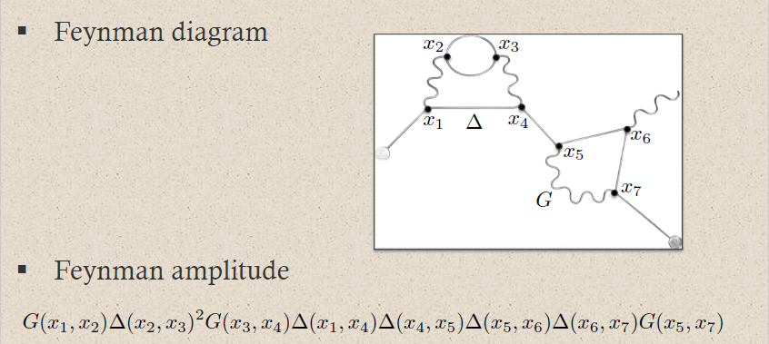 | Moyal product for Feynman propagator |
We now discuss Feynman diagrams and their Feynman amplitudes in two stages: First we consider plain finite multigraphs with linearly ordered vertices but no other labels (def. below) and discuss how these generally organize an expansion of the time-ordered products as a sum of distributional products of the given Feynman propagator (prop. below). These summands (or their vacuum expectation values) are called the Feynman amplitudes if one thinks of the underlying free field vacuum as having a single “field species” and of the chosen interaction to be a single “interaction vertex”.
But often it is possible and useful to identify different field species and different interaction vertices. In fact in applications this choice is typically evident and not highlighted as a choice. We make it explicit below as def. . Such a choice makes both the interaction term as well as the Feynman propagator decompose as sums (remark below). Accordingly then, after “multiplying out” the products of these sums that appear in the Feynman amplitudes, these, too, decompose further as as sums indexed by multigraphs whose edges are labeled by field species, and whose vertices are labeled by interactions. These labeled multigraphs are the Feynman diagrams (def. below) and the corresponding summands are the Feynman amplitudes proper (prop. below).
Definition
A finite multigraph is
-
a finite set (“of vertices”);
-
a finite set (“of edges”);
-
a function
(sending any edge to the unordered pair of distinct vertices that it goes between).
A choice of linear order on the set of vertices of a finite multigraph is a choice of bijection of the form
Hence the isomorphism classes of a finite multigraphs with linearly ordered vertices are characterized by
-
(the number of vertices);
-
for each a natural number
(the number of edges between the th and the th vertex).
We write for the set of such isomorphism classes of finite multigraphs with linearly ordered vertices identified with ; and we write
for the set of isomorphism classes of finite multigraphs with linearly ordered vertices of any number.
Proposition
(Feynman amplitudes of finite multigraphs)
Let be a relativistic free vacuum according to def. .
For , the -fold time-ordered product away from coinciding interaction points, given by prop.
is equal to the following formal power series labeled by isomorphism classes of finite multigraphs with linearly ordered vertices, (def. ):
where is, for short, the number of edges between vertex and vertex in the finite multigraph of the outer sum, according to def. .
Here the summands of the expansion (23)
and/or their vacuum expectation values
are called the Feynman amplitudes for scattering processes in the given free field vacuum of shape with interaction vertices . Their expression as products of distributions via algebraic expression on the right hand side of (24) is also called the Feynman rules.
Proof
We proceed by induction over the number of vertices. The statement is trivially true for a single vertex. So assume that it is true for vertices. It follows that
The combinatorial factor over the brace is the multinomial coefficient expressing the number of ways of distributing -many functional derivatives to factors, via the product rule, and quotiented by the factorial that comes from the exponential in the definition of the star product.
Here in the first step we used the associativity (19) of the restricted time-ordered product, in the second step we used the induction assumption, in the third we passed the outer functional derivatives through the pointwise product using the product rule, and in the fourth step we recognized that this amounts to summing in addition over all possible choices of sets of edges from the first vertices to the new st vertex, which yield in total the sum over all diagrams with vertices.
If the free field theory is decomposed as a direct sum of free field theories, we obtain a more fine-grained concept of Feynman amplitudes:
Definition
(field species and interaction vertices)
Let be a relativistic free vacuum according to def. , and let be a local observable regarded as an adiabatically switched interaction action functional.
Then
-
a choice of field species is a choice of decomposition of the BV-BRST field bundle as a fiber product over finite set of (graded super-) field bundles
such that the gauge fixed free Lagrangian density is the sum
on these separate field bundles.
-
a choice of interaction vertices and external vertices is a choice of sum decomposition
parameterized by finite sets and , to be called the sets of internal vertex labels and external vertex labels, respectively.
Remark
(Feynman propagator for separate field species)
Let be a relativistic free vacuum according to def. .
Then a choice of field species as in def. induces a corresponding decomposition of the Feynman propagator of the gauge fixed free field theory
as the sum of Feynman propagators for each of the chosen field species:
hence in components, with the collective field coordinates on , this decomposition is of the form
Example
(field species in quantum electrodynamics)
The field bundle for Lorenz gauge fixed quantum electrodynamics on Minkowski spacetime admits a decomposition into field species, according to def. , as
(by this example and this example).
The corresponding sum decomposition of the Feynman propagator, according to remark , is
where
-
is the electron propagator (this def.)
-
is the photon propagator in Gaussian-averaged Lorenz gauge (this prop.)
-
the ghost field and antighost field Feynman propagators , and are each one copy of the Feynman propagator of the real scalar field (this prop.), while the Nakanishi-Lautrup field contributes a mixing with the photon propagator, notationally suppressed behind the star-symbols above.
Definition
Let be a relativistic free vacuum according to def. , and let be a local observable regarded as an adiabatically switched interaction action functional.
Let moreover
be a choice of field species, according to def ,
a choice of internal and external interaction vertices according to def. .
With these choices, we say that a Feynman diagram is
-
a finite multigraph with linearly ordered vertices (def. )
-
to the disjoint union of the chosen sets of internal and external vertex labels;
-
to the chosen set of field species.
We write
for the set of isomorphism classes of Feynman diagrams with labels in , refining the set of isomorphisms of plain finite multigraphs with linearly ordered vertices from def. .
Proposition
(Feynman amplitudes for Feynman diagrams)
Let be a relativistic free vacuum according to def. , and let be a local observable regarded as an adiabatically switched interaction action functional.
Let moreover
be a choice of field species, according to def , hence inducing, by remark , a sum decomposition of the Feynman propagator
and let
be a choice of internal and external interaction vertices according to def. .
Then by “multiplying out” the products of the sums (25) and (26) in the formula (24) for the Feynman amplitude (def. ) this decomposes as a sum of the form
over all ways of labeling the vertices of by the internal or external vertex labels, and the edges of by field species. The corresponding summands
or rather their vacuum expectation value
are called the Feynman amplitude associated with these Feynman diagrams.
Example
(Feynman amplitudes in causal perturbation theory – example of QED)
In perturbative quantum field theory, Feynman diagrams are labeled multigraphs that encode products of Feynman propagators, called Feynman amplitudes (this prop.) which in turn contribute to probability amplitudes for physical scattering processes – scattering amplitudes:
The Feynman amplitudes are the summands in the Feynman perturbation series-expansion of the scattering matrix
of a given interaction Lagrangian density .
The Feynman amplitudes are the summands in an expansion of the time-ordered products of the interaction with itself, which, away from coincident vertices, is given by the star product of the Feynman propagator (this prop.), via the exponential contraction
Each edge in a Feynman diagram corresponds to a factor of a Feynman propagator in , being a distribution of two variables; and each vertex corresponds to a factor of the interaction Lagrangian density at .
For example quantum electrodynamics in Gaussian-averaged Lorenz gauge involves (via this example):
-
the Dirac field modelling the electron, with Feynman propagator called the electron propagator (this def.), here to be denoted
-
the electromagnetic field modelling the photon, with Feynman propagator called the photon propagator (this prop.), here to be denoted
The Feynman diagram for the electron-photon interaction alone is
where the solid lines correspond to the electron, and the wiggly line to the photon. The corresponding product of distributions is (written in generalized function-notation)
Hence a typical Feynman diagram in the QED Feynman perturbation series induced by this electron-photon interaction looks as follows:
where on the bottom the corresponding Feynman amplitude product of distributions is shown; now notationally suppressing the contraction of the internal indices and all prefactors.
For instance the two solid edges between the vertices and correspond to the two factors of :
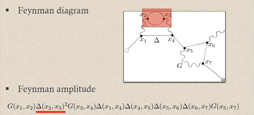
This way each sub-graph encodes its corresponding subset of factors in the Feynman amplitude:
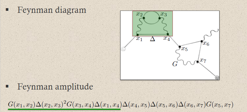
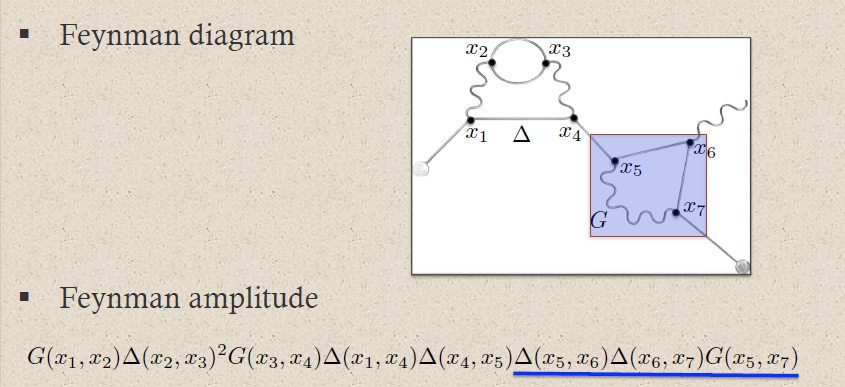
graphics grabbed from Brouder 10
A priori this product of distributions is defined away from coincident vertices: . The definition at coincident vertices requires a choice of extension of distributions to the diagonal locus. This choice is the ("re-")normalization of the Feynman amplitude.
Example
Let be a relativistic free vacuum according to def. , and let
be a local observable, regarded as a adiabatically switched interaction action functional.
By prop. every choice of perturbative S-matrix (def. )
has an expansion as a formal power series of the form
where the series is over all finite multigraphs with linearly ordered vertices (def. ), and the summands are the corresponding ("re"-)normalized (def. ) Feynman amplitudes (prop. ).
If moreover a choice of field species and of internal and external interaction vertices is made, according to def. , then this series expansion refines to an expansion over all Feynman diagrams (def. ) of Feynman amplitudes (def. ):
Expressed in this form the S-matrix is known as the Feynman perturbation series.
Remark
(no tadpole Feynman diagrams)
In the definition of finite multigraphs in def. there are no edges considered that go from any vertex to itself. Accordingly, there are no such labeled edges in Feynman diagrams (def. ):

In pQFT these diagrams are called tadpoles, and their non-appearance is considered part of the Feynman rules (prop. ). Via prop. this condition reflects the nature of the star product (this def.) which always contracts different tensor product factors with the Feynman propagator before taking their pointwise product.
Beware that in graph theory these tadpoles are called “loops”, while here in pQFT a “loop” in a planar graph refers instead to what in graph theory is called a face of the graph, see the discussion of loop order in prop. below.
(Keller 10, remark II.8 and proof of prop. II.7)
Effective action
We have seen that the Feynman perturbation series expresses the S-matrix as a formal power series of Feynman amplitudes labeled by Feynman diagrams. Now the Feynman amplitude associated with a disjoint union of connected Feynman diagrams (def. below) is just the product of the amplitudes of the connected components (prop. below). This allows to re-organize the Feynman perturbation series as the ordinary exponential of the Feynman perturbation series restricted to just connected Feynman diagrams. The latter is called the effective action (def. below) because it allows to express vacuum expectation values of the S-matrix as an ordinary exponential (equation (28) below).
Definition
Given two finite multigraphs (def. ), their disjoint union
is the finite multigraph whose set of vertices and set of edges are the disjoint unions of the corresponding sets of and
and whose vertex-assigning function is the corresponding function on disjoint unions
The operation induces a pairing on the set of isomorphism classes of finite multigraphs
A finite multigraph (def. ) is called connected if it is not the disjoint union of two non-empty finite multigraphs.
We write
for the subset of isomorphism classes of connected finite multigraphs.
Lemma
(Feynman amplitudes multiply under disjoint union of graphs)
Let
be disjoint union of graphs (def. ). then then corresponding Feynman amplitudes (prop. ) multiply by the pointwise product (this def.):
Proof
By prop. the contributions to the S-matrix away from coinciding interaction points are given by the star product induced by the Feynman propagator, and specifically, by prop. , the Feynman amplitudes are given this way. Moreover the star product (this def.) is given by first contracting with powers of the Feynman propagator and then multiplying all resulting terms with the pointwise product of observables. This implies the claim by the nature of the combinatorial factor in the definition of the Feynman amplitudes (prop. ).
Definition
Let be a relativistic free vacuum according to def. , let be an S-matrix scheme for perturbative QFT around this vacuum (def. ) and let
be a local observable.
Recall that for each finite multigraph (def. ) the Feynman perturbation series for (example )
contributes with a ("re"-)nromalized Feynman amplitude .
We say that the corresponding effective action is times the sub-series
of Feynman amplitudes that are labeled only by the connected graphs (def. ).
(A priori could contain negative powers of , but it turns out that it does not; this is prop. below.)
Remark
(terminology for “effective action”)
Beware differing conventions of terminology:
-
In effective quantum field theory, the effective action in def. is sometimes called the effective potential at scale (see this prop.).
This terminology originates in restriction to the special example of the scalar field, where the typical non-derivative Phi^n interactions are naturally thought of as potential energy-terms.
From this perspective the effective action in def. is a special case of relative effective actions (“relative effective potentials”, in the case of Phi^n interactions) relative to an arbitrary UV cutoff-scales (this def.).
-
For the special case that
is a regular linear observable (this def.) the effective action according to def. is often denoted or , and then its functional Legendre transform (if that makes sense) is instead called the effective action, instead.
This is because the latter encodes the equations of motion for the vacuum expectation values of the interacting field observables; we discuss this as example below.
Notice the different meaning of “effective” in both cases: In the first case it refers to what is effectively seen of the full pQFT at some UV-cutoff scale, while in the second case it refers to what is effectively seen when restricting attention only to the vacuum expectation values of regular linear observables.
Proposition
(effective action is logarithm of S-matrix)
Let be a relativistic free vacuum according to def. , let be an S-matrix scheme for perturbative QFT around this vacuum (def. ) and let
be a local observable and let
be the corresponding effective action (def. ).
Then then S-matrix for is the exponential of the effective action with respect to the pointwise product of observables (this def.):
Moreover, this relation passes to the vacuum expectation values:
Conversely the vacuum expectation value of the effective action is to the logarithm of that of the S-matrix:
Proof
By lemma the summands in the th pointwise power of times the effective action are precisely the Feynman amplitudes of finite multigraphs with connected components, where each such appears with multiplicity given by the factorial of :
It follows that
yields the Feynman perturbation series by expressing it as a series (re-)organized by number of connected components of the Feynman diagrams.
To conclude the proof it is now sufficient to observe that taking vacuum expectation values of polynomial observables respects the pointwise product of observables
This is because the Hadamard vacuum state simply picks the zero-order monomial term, by this prop., and under multiplication of polynomials the zero-order terms are multiplied.
This immediately implies the following important fact:
Proposition
(in stable vacuum the effective action is generating function for vacuum expectation values of interacting field observables)
Let be a relativistic free vacuum according to def. , and let be a local observable regarded as an adiabatically switched interaction action functional.
If the given vacuum state is stable (def. ) then the vacuum expectation value of the effective action (def. ) is the generating function for the vacuum expectation value of the interacting field observable (def. ) in that
Proof
We compute as follows:
Here in the first step we used prop , in the second step we applied the chain rule of differentiation, in the third step we used the definition of vacuum stability (def. ) and in the fourth step we recognized the definition of the interacting field observables (def. ).
Example
(equations of motion for vacuum expectation values of interacting field observables)
Consider the effective action (def. ) for the case that
is a regular linear observable (this def.), hence the smearing of a field observable (this def.) by an adiabatic switching of the source field
(Here we are notationally suppressing internal field indices, for convenience.)
In this case the vacuum expectation value of the corresponding effective action is often denoted
and regarded as a functional of the adiabatic switching of the source field.
In this case prop. says that if the vacuum state is stable, then is the generating functional for interacting (def. ) field observables (this def.) in that
Assume then that there exists a corresponding functional of the field histories , which behaves like a functional Legendre transform of in that it satisfies the functional version of the defining equation of Legendre transforms (first derivatives are inverse functions of each other, see this equation), in that
By (29) this implies that
This may be read as a quantum version of the principle of extremal action (this prop.) formulated now not for the field histories , but for the vacuum expectation values of their corresponding interacting quantum field observables.
Beware, (as in remark ) that many texts refer to as the effective action, instead of its Legendre transform, the generating functional .
The perspective of the effective action also gives a transparent picture of the order of quantum effects involved in the S-matrix, this is prop. below. In order to state this conveniently, we invoke two basic concepts from graph theory:
Definition
(planar graphs and trees)
A finite multigraph (def. ) is called a planar graph if it admits an embedding into the plane, hence if it may be “drawn into the plane” without intersections, in the evident way.
A finite multigraph is called a tree if for any two of its vertices there is at most one path of edges connecting them, these are examples of planar graphs. We write
for the subset of isomorphism classes of finite multigraphs with linearly orrdered vertices (def. ) on those which are trees.
Proposition
(loop order and tree level of Feynman perturbation series)
The effective action (def. ) contains no negative powers of , hence is indeed a formal power series also in :
and in particular
Moreover, the contribution to the effective action in the classical limit is precisely that of Feynman amplitudes of those finite multigraphs (prop. ) which are trees (def. ); thus called the tree level-contribution:
Finally, a finite multigraph (def. ) which is planar (def. ) and connected (def. ) contributes to the effective action precisely at order
where is the number of faces of , here called the number of loops of the diagram; here usually called the loop order of .
(Beware the terminology clash with graph theory, see the discussion of tadpoles in remark .)
Proof
By def. the explicit -dependence of the S-matrix is
and by prop. the further -dependence of the time-ordered product is
By the Feynman rules (prop. ) this means that
-
each vertex of a Feynman diagram contributes a power to its Feynman amplitude;
-
each edge of a Feynman diagram contributes a power to its Feynman amplitude.
If we write
for the total number of vertices and edges, respectively, in , this means that a Feynman amplitude corresponding to some contributes precisely at order
So far this holds for arbitrary . If however is connected (def. ) and planar (def. ), then Euler's formula asserts that
Hence is the order of at which contributes to the scattering matrix expressed as the Feynman perturbation series.
But the effective action, by definition (27), has the same contributions of Feynman amplitudes, but multiplied by another power of , hence it contributes at order
This proves the second claim on loop order.
The first claim, due to the extra factor of in the definition of the effective action, is equivalent to saying that the Feynman amplitude of every connected finite multigraph contributes powers in of order and contributes at order precisely if the graph is a tree.
Observe that a connected finite multigraph with vertices (necessarily ) has at least edges and precisely edges if it is a tree.
To see this, consecutively remove edges from as long as possible while retaining connectivity. When this process stops, the result must be a connected tree , hence a connected planar graph with . Therefore Euler's formula (31) implies that that .
This means that the connected multigraph in general has a Feynman amplitude of order
and precisely if it is a tree its Feynman amplitude is of order .
Vacuum diagrams
With the Feynman perturbation series and the effective action in hand, it is now immediate to see that there is a general contribution by vacuum diagrams (def. below) in the scattering matrix which, in a stable vacuum state, cancels out against the prefactor in Bogoliubov's formula for interacting field observables.
Definition
Let be a relativistic free vacuum according to def. , and let be a local observable regarded as an adiabatically switched interaction action functional, and consider a choice of decomposition for field species and interaction vertices according to def. .
Then a Feynman diagram all whose vertices are internal vertices (def. ) is called a vacuum diagram.
Write
for the subset of isomorphism classes of vacuum diagrams among the set of isomorphism classes of all Feynman diagrams, def. . Similarly write
for the subset of isomorphism classes of Feynman diagrams which are both vacuum diagrams as well as connected graphs (def. ).
Finally write
for the sub-series of that for the effective action (def. ) given only by those connected diagrams which are also vacuum diagrams.
Example
(2-vertex vacuum diagram in QED)
The vacuum diagram (def. ) with two electron-photon interaction-vertices in quantum electrodynamics (this example.) is:
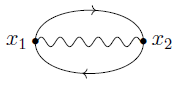
Example
(vacuum diagram-contribution to S-matrices)
Let be a relativistic free vacuum according to def. , and let be a local observable regarded as an adiabatically switched interaction action functional, and consider a choice of decomposition for field species and interaction vertices according to def. .
Then the Feynman perturbation series-expansion of the S-matrix (example ) of the interaction-term alone (no source field-contribution) is the series of Feynman amplitudes that are labeled by vacuum diagrams (def. ), hence (by prop. ) the exponential of the vacuum effective action (def. ):
More generally, the S-matrix with source field-contribution included always splits as a pointwise product of the vacuum S_matrix with the Feynman perturbation series over all Feynman graphs with at least one external vertex:
Hence if the free field vacuum state is stable with respect to the interaction , according to def. , then the vacuum expectation value of a time-ordered product of interacting field observables (example ) and hence in particular of scattering amplitudes (example ) is given by the Feynman perturbation series (example ) over just the non-vacuum Feynman diagrams, hence over all those diagram that have at least one one external vertex
This is the way in which the Feynman perturbation series is used in practice for computing scattering amplitudes.
Interacting quantum BV-Differential
So far we have discussed, starting with a BV-BRST gauge fixed free field vacuum, the perturbative construction of interacting field algebras of observables (def. ) and their organization in increasing powers of and (loop order, prop. ) via the Feynman perturbation series (example , example ).
But this interacting field algebra of observables still involves all the auxiliary fields of the BV-BRST gauge fixed free field vacuum (as in example for QED), while the actual physical gauge invariant on-shell observables should be (just) the cochain cohomology of the BV-BRST differential on this enlarged space of observables. Hence for the construction of perturbative QFT to conclude, it remains to pass the BV-BRST differential of the free field Wick algebra of observables to a differential on the interacting field algebra, such that its cochain cohomology is well defined.
Since the time-ordered products away from coinciding interaction points and as well as on regular polynomial observables are uniquely fixed (prop. ), one finds that also this interacting quantum BV-differential is uniquely fixed, on regular polynomial observables, by conjugation with the quantum Møller operators (def. ). The formula that characterizes it there is called the quantum master equation or equivalently the quantum master Ward identity (prop. below).
When extending to coinciding interaction points via ("re"-)normalization (def. ) these identities are not guaranteed to hold anymore, but may be imposed as renormalization conditions (def. , prop. ). Quantum correction to the master Ward identity then imply corrections to Noether current conservation laws; this we discuss below.
Recall how the global BV-differential
on regular polynomial observables (this def.) is conjugated into the time-ordered product via the time ordering operator (this prop.).
In the same way we may use the quantum Møller operators to conjugate the BV-differential into the regular part of the interacting field algebra of observables:
Definition
(interacting quantum BV-differential)
Given an adiabatically switched non-point-interaction action functional in the form of a regular polynomial observable , then the interacting quantum BV-differential on the interacting field algebra (def. ) on regular polynomial observables is the conjugation of the plain BV-differential by the quantum Møller operator induced by (def. ):
Proposition
(quantum master equation and quantum master Ward identity on regular polynomial observables)
Consider an adiabatically switched non-point-interaction action functional in the form of a regular polynomial observable in degree 0
Then the following are equivalent:
-
The quantum master equation (QME)
(32) -
The perturbative S-matrix (def. ) is -closed
-
The quantum master Ward identity (MWI) on regular polynomial observables in terms of retarded products:
(33)expressing the interacting quantum BV-differential (def. ) as the sum of the time-ordered antibracket (this def.) with the total action functional and times the BV-operator (BV-operator).
-
The quantum master Ward identity (MWI) on regular polynomial observables in terms of time-ordered products:
(34)
(Rejzner 11, (5.35) - (5.38), following Hollands 07, (342)-(345))
Proof
To see that the first two conditions are equivalent, we compute as follows
Here in the first step we used the definition of the BV-operator (this def.) to rewrite the plain antibracket in terms of the time-ordered antibracket (this def.), then under the second brace we used that the time-ordered antibracket is the failure of the BV-operator to be a derivation (this prop) and under the first brace the consequence of this statement for application to exponentials (this example). Finally we collected terms, and to “complete the square” we added the terms on the left of
which vanish because, by definition of gauge fixing (this def.), the free gauge-fixed action functional is independent of antifields.
But since the operation has the inverse , this implies the claim.
Next we show that the quantum master equation implies the quantum master Ward identities.
We use that the BV-differential is a derivation of the Wick algebra product (lemma ).
First of all this implies that with also .
Thus we compute as follows:
By applying to both sides of this equation, this means first of all that the interacting quantum BV-differential is equivalently given by
hence that if either version (33) or (37) of the master Ward identity holds, it implies the other.
Now expanding out the definition of (def. ) and expressing via the time-ordered antibracket (this def.) and the BV-operator (this prop.) as
(on regular polynomial observables), we continue computing as follows:
Here in the line with the braces we used that the BV-operator is a derivation of the time-ordered product up to correction by the time-ordered antibracket (this prop.), and under the first brace we used the effect of that property on time-ordered exponentials (this example), while under the second brace we used that is a derivation of the time-ordered product. Finally we have collected terms, added as before, and then used the QME.
This shows that the quantum master Ward identities follow from the quantum master equation. To conclude, it is now sufficient to show that, conversely, the MWI in terms of, say, retarded products implies the QME.
To see this, observe that with the BV-differential being nilpotent, also its conjugation by is, so that with the above we have:
Here under the brace we computed as follows:
where, in turn, the term under the first brace follows by the graded Jacobi identity, the one under the second brace by Henneaux-Teitelboim (15.105c) and the one under the third brace by Henneaux-Teitelboim (15.105b).
Ward identities
The quantum master Ward identity (prop. ) expresses the relation between the quantum (measured by Planck's constant ) interacting (measured by the coupling constant ) equations of motion to the classical free field equations of motion at (remark below). As such it generalizes the Schwinger-Dyson equation (this prop.), to which it reduces for (example below) as well as the classical master Ward identity, which is the case for (example below).
Applied to products of the equations of motion with any given observable, the master Ward identity becomes a particular Ward identity.
This is of interest notably in view of Noether's theorem (this prop.), which says that every infinitesimal symmetry of the Lagrangian of, in particular, the given free field theory, corresponds to a conserved current (this def.), hence a horizontal differential form whose total spacetime derivative vanishes up to a term proportional to the equations of motion. Under transgression to local observables this is a relation of the form
where “on shell” means up to the ideal generated by the classical free equations of motion. Hence for the case of local observables of the form , the quantum Ward identity expresses the possible failure of the original conserved current to actually be conserved, due to both quantum effects () and interactions (). This is the form in which Ward identities are usually understood (example below).
As one extends the time-ordered products to coinciding interaction points in ("re"-)normalization of the perturbative QFT (def. ), the quantum master equation/master Ward identity becomes a renormalization condition (def. , prop. ). If this condition fails, one speaks of a quantum anomaly. Specifically if the Ward identity for an infinitesimal gauge symmetry is violated, one speaks of a gauge anomaly.
Definition
Consider a free gauge fixed Lagrangian field theory (this def.) with global BV-differential on regular polynomial observables
(this def.).
Let moreover
be a regular polynomial observable (regarded as an adiabatically switched non-point-interaction action functional) such that the total action satisfies the quantum master equation (this prop.); and write
for the corresponding quantum Møller operator (this def.).
Then by this prop. we have
This is the quantum master Ward identity on regular polynomial observables, i.e. before renormalization.
Remark
(quantum master Ward identity relates quantum interacting field EOMs to classical free field EOMs)
For the quantum master Ward identity on regular polynomial observables (37) reads
The term on the right is manifestly in the image of the global BV-differential of the free field theory (this def.) and hence vanishes when passing to on-shell observables along the isomorphism (this equation)
(by this example).
Hence
In contrast, the left hand side is the interacting field observable (via this def.) of the sum of the time-ordered antibracket with the action functional of the interacting field theory and a quantum correction given by the BV-operator. If we use the definition of the BV-operator (this def.) we may equivalently re-write this as
Hence the quantum master Ward identity expresses a relation between the ideal spanned by the classical free field equations of motion and the quantum interacting field equations of motion.
Example
(free field-limit of master Ward identity is Schwinger-Dyson equation)
In the free field-limit (noticing that in this limit ) the quantum master Ward identity (37) reduces to
which is the defining equation for the BV-operator (this equation), hence is isomorphic (under ) to the Schwinger-Dyson equation (this prop.)
Example
(classical limit of quantum master Ward identity)
In the classical limit (noticing that the classical limit of is ) the quantum master Ward identity (37) reduces to
This says that the interacting field observable corresponding to the global antibracket with the action functional of the interacting field theory vanishes on-shell, classically.
Applied to an observable which is linear in the antifields
this yields
This is the classical master Ward identity according to (Dütsch-Fredenhagen 02, Brennecke-Dütsch 07, (5.5)), following (Dütsch-Boas 02).
Example
(quantum correction to Noether current conservation)
Let be an evolutionary vector field, which is an infinitesimal symmetry of the Lagrangian , and let the corresponding conserved current, by Noether's theorem I (this prop.), so that
(by this equation), where in the second line we just rewrote the expression in components (using this equation)
and re-arranged suggestively.
Then for any choice of bump function, we obtain the local observables
and
by transgression of variational differential forms.
This is such that
Hence applied to this choice of local observable , the quantum master Ward identity (39) now says that
Hence the interacting field observable-version of need not vanish itself on-shell, instead there may be a correction as shown on the right.
Retarded products
We have seen that the exponential series-expansion of the perturbative S-matrix is given by “time-ordered products”. Similarly there is an exponential series-expansion of the quantum Møller operator (def. ); its coefficients are called the retarded products (def. ) below.
Hence where the time-ordered products directly relate to scattering amplitudes (example ) the retarded products directly relate to more general interacting field observables (def. ).
The formulation of interacting field theory via time-ordered products or retarded products is essentially equivalent; in any given situation either one may be more conenient than the other.
Definition
(retarded products from S-matrix)
It follows from the perturbation axiom in def. that there is a system of continuous linear functionals
for all such that
Similarly there is
These are called the (generating) retarded products (Glaser-Lehmann-Zimmermann 57, Epstein-Glaser 73, section 8.1).
Direct axiomatization of the retarded products is due to (Dütsch-Fredenhagen 04), see (Collini 16, section 2.2).
(…)
In functorial quantum field theory
At least the idea of the S-matrix is very explicit in the Atiyah-Segal picture of functorial QFT (FQFT).
Here a quantum field theory is given by a functor
from a suitable category of cobordisms to a suitable category of vector spaces.
-
To a codimension-1 slice of space this assigns a vector space – the (Hilbert) space of quantum states over ;
-
to a spacetime/worldvolume manifold with boundaries one assigns the quantum propagator which is the linear map that takes incoming states to outgoing states via propagation along the spacetime/worldvolume . This is alternatively known as the the scattering amplitude or S-matrix for propagation from to along a process of shape .
Now for genuine topological field theories all spaces of quantum states are finite dimensional and hence we can equivalently consider the dual vector space (using that finite dimensional vector spaces form a compact closed category). Doing so the propagator map
equivalently becomes a linear map of the form
Notice that such a linear map from the canonical 1-dimensional complex vector space to some other vector space is equivalently just a choice of element in that vector space. It is in this sense that is equivalently a vector in .
In this form in physics the propagator is usually called the correlator or n-point function .
Segal’s axioms for FQFT (CFT in his case) were originally explicitly about the propagators/S-matrices, while Atiyah formulated it in terms of the correlators this way. Both perspectives go over into each other under duality as above.
Notice that this kind of discussion is not restricted to topological field theory. For instance already plain quantum mechanics is usefully formulated this way, that’s the point of finite quantum mechanics in terms of dagger-compact categories.
Properties
Possible symmetries
see at Haag–Lopuszanski–Sohnius theorem
Examples
Chern-Simons theory
The Feynman amplitudes of higher Chern-Simons theory, such as AKSZ sigma-models, regarded in their incarnation as Feynman amplitudes on compactified configuration spaces of points, serve to exhibit a graph complex-model for the de Rham complex of Fulton-MacPherson compactifications of configuration spaces of points by the construction recalled there. See the pointers at Chern-Simons theory here.
History
In the 1960s there was a prominent proposal, around Geoffrey Chew, that (perturbative) quantum field theory should be defined by axiomatizing properties of the S-matrix without explicit reference to fields on spacetime.
Here analycity (or more general the crossing property) of the S-matrix reflects its causal factorization, and hence this is often referred to as the analytic S-matrix (see Eden-Ladshoff-Olive-Polkinhorne 66).
This is a radical perspective where no spacetime geometry and physical fields are made explicit, but where the entire physics is encoded by what quantum particles see that scatter through it.
Historically, this S-matrix “bootstrap” approach fell out of fashion with the success of the quark model in quantum chromodynamics, which is a local Lagrangian field theory (Yang-Mills theory) defined in terms of fields on spacetime.
See also the discussion in (Chew 70, Schroer 11).
But later perturbative string theory revived the axiomatic S-matrix perspective. In general, perturbative string theory is not defined by a geometric spacetime background. Instead the background is algebraically encoded by a 2d SCFT (“2-spectral triple”) and the string perturbation series is a formula that translates this into an S-matrix. Spacetime physics then is whatever is seen by string scattering processes (see also at string theory FAQ – What are the equations of string theory?).
More recently, the S-matrix perspective becomes fashionable also in Yang-Mills theory, with people noticing that super Yang-Mills theory and Tr(ϕ³) enjoy good structures in its scattering amplitudes which are essentially invisible in the vast summation of Feynman diagrams that extract the S-matrix from the action functional. Instead there are entirely different mathematical structures that encode at least some sub-class of scattering amplitudes (see at amplituhedron and associahedron). This has lead to increasingly close ties between the S-matrix program and the mathematical fields of geometry and combinatorics, allowing for the development of various other structures in quantum field theory that encode, for instance, the Wheeler-wavefunction of the universe (see at cosmohedron) and the UV/IR divergence of Feynman integrals (see at Feynman polytope).
From this physics.SE comment by Ron Maimon:
The history of physics cannot be well understood without appreciating the unbelievable antagonism between the Chew/Mandelstam/Gribov S-matrix camp, and the Weinberg/Glashow/Polyakov Field theory camp. The two sides hated each other, did not hire each other, and did not read each other, at least not in the west. The only people that straddled both camps were older folks and Russians— Gell-Mann more than Landau (who believed the Landau pole implied the S-matrix), Gribov and Migdal more than anyone else in the west other than Gell-Mann and Wilson. Wilson did his PhD in S-matrix theory, for example, as did David Gross (under Chew).
In the 1970s, S-matrix theory just plain died. All practitioners jumped ship rapidly in 1974, with the triple-whammy of Wilsonian field theory, the discovery of the Charm quark, and asymptotic freedom. These results killed S-matrix theory for thirty years. Those that jumped ship include all the original string theorists who stayed employed: notably Veneziano, who was convinced that gauge theory was right when t'Hooft showed that large-N gauge fields give the string topological expansion, and Susskind, who didn’t mention Regge theory after the early 1970s. Everybody stopped studying string theory except Scherk and Schwarz, and Schwarz was protected by Gell-Mann, or else he would never have been tenured and funded.
This sorry history means that not a single S-matrix theory course is taught in the curriculum today, nobody studies it except a few theorists of advanced age hidden away in particle accelerators, and the main S-matrix theory, string theory, is not properly explained and remains completely enigmatic even to most physicists. There were some good reasons for this — some S-matrix people said silly things about the consistency of quantum field theory — but to be fair, quantum field theory people said equally silly things about S-matrix theory.
Weinberg came up with these heuristic arguments in the 1960s, which convinced him that S-matrix theory was a dead end, or rather, to show that it was a tautological synonym for quantum field theory. Weinberg was motivated by models of pion-nucleon interactions, which was a hot S-matrix topic in the early 1960s. The solution to the problem is the chiral symmetry breaking models of the pion condensate, and these are effective field theories.
Building on this result, Weinberg became convinced that the only real solution to the S-matrix was a field theory of some particles with spin. He still says this every once in a while, but it is dead wrong. The most charitable interpretation is that every S-matrix has a field theory limit, where all but a finite number of particles decouple, but this is not true either (consider little string theory). String theory exists, and there are non-field theoretic S-matrices, namely all the ones in string theory, including little string theory in (5+1)d, which is non-gravitational.
From (Weinberg 09, p. 11):
I offered this in my 1979 paper as what Arthur Wightman would call a folk theorem: “if one writes down the most general possible Lagrangian, including all terms consistent with assumed symmetry principles, and then calculates matrix elements with this Lagrangian to any given order of perturbation theory, the result will simply be the most general possible S-matrix consistent with perturbative unitarity, analyticity, cluster decomposition, and the assumed symmetry properties.”
There was an interesting irony in this. I had been at Berkeley from 1959 to 1966, when Geoffrey Chew and his collaborators were elaborating a program for calculating S-matrix elements for strong interaction processes by the use of unitarity, analyticity, and Lorentz invariance, without reference to quantum field theory. I found it an attractive philosophy, because it relied only on a minimum of principles, all well established. Unfortunately, the S-matrix theorists were never able to develop a reliable method of calculation, so I worked instead on other things, including current algebra. Now in 1979 I realized that the assumptions of S-matrix theory, supplemented by chiral invariance, were indeed all that are needed at low energy, but the most convenient way of implementing these assumptions in actual calculations was by good old quantum field theory, which the S-matrix theorists had hoped to supplant.
Related entries
-
scattering amplitude, Feynman diagram, string scattering amplitude,
-
string theory FAQ – What are the equations of string theory?
See also at sigma model the section Exposition of second quantization of sigma-models
References
General
Early work basing perturbative quantum field theory on the concept of the S-matrix is
- Werner Heisenberg, Die “beobachtbaren Größen” in der Theorie der Elementarteilchen, Zeitschrift für Physik 120, 513, 1943 (doi:10.1007/978-3-642-70078-1_44)
recalled in
- Alexander S. Blum, The state is not abolished, it withers away: how quantum field theory became a theory of scattering (arXiv:2011.05908)
This proposal was vocally promoted as the “bootstrap program” by Geoffrey Chew and Stanley Mandelstam (see Chew 70).
An account of the history of the contributions by Tullio Regge is in
- Alessandro Bottino, A retrospective look at Regge poles (arXiv:1807.02456)
On the history of the S-matrix in view of the origin of string theory:
- Robert van Leeuwen, From S-matrix theory to strings: Scattering data and the commitment to non-arbitrariness [arXiv:2403.06690]
Textbook accounts of this axiomatic approach to defining the S-matrix (i.e. not proceeding via Lagrangian field theory but via analyticity axioms):
-
Eden, Landshoff, David Olive, John Polkinghorne, The Analytic S-matrix, Cambridge 1966 (pdf)
-
Vladimir Gribov, The theory of complex angular momenta, Lecture St. Petersburg 1996, publsihed. Cambridge 2003 (doi:10.1017/CBO9780511534959)
-
Franco Strocchi, §6 of: An Introduction to Non-Perturbative Foundations of Quantum Field Theory, Oxford University Press (2013) [doi:10.1093/acprof:oso/9780199671571.001.0001]
Exposition and review (with modern relation to conformal bootstrap):
- Sebastian Mizera, Physics of the Analytic S-Matrix [arXiv:2306.05395]
Discussion of S-matrix analyticity as a constraint on global causality violation of locally Lorentz invariant theories:
- Allan Adams, Nima Arkani-Hamed, Sergei Dubovsky, Alberto Nicolis, Riccardo Rattazzi, Causality, Analyticity and an IR Obstruction to UV Completion, JHEP 0610:014, 2006 (arXiv:hep-th/0602178)
General discussion of scattering theory:
-
Roger G. Newton, Scattering Theory of Waves and Particles, Springer 1982 (TOC pdf)
-
Daniel Iagolnitzer, The Analyticity Program in Axiomatic Quantum Field Theory, in A.B. de Monvel, Detlev Buchholz, Daniel Iagolnitzer, Moschella U. (eds.) Rigorous Quantum Field Theory, Progress in Mathematics, vol 251. Birkhäuser, Basel, 2007, (web)
-
Daniel Iagolnitzer, Scattering in Quantum Field Theories, The Axiomatic and Constructive Approaches, Princeton 2014 (web)
A textbook account of the traditional heuristic picture deriving the S-matrix in perturbative Lagrangian field theory is in
- Steven Weinberg, chapter 3 of The quantum theory of fields - Volume I: Foundations, Cambridge 1995
The mathematically rigorous construction of the S-matrix in perturbative Lagrangian field theory via causal perturbation theory is due to
- Henri Epstein, Vladimir Glaser, The Role of locality in perturbation theory, Annales Poincaré Phys. Theor. A 19 (1973) 211 (Numdam)
based on ideas due to (Stückelberg 49, Stückelberg 51) and
- Nikolay Bogoliubov, Dmitry Shirkov, Introduction to the Theory of Quantized Fields, New York (1959)
Comparative discussion of the two perspectives on the S-matrix includes:
-
Geoffrey Chew, Quark or Bootstrap: Triumph or Frustration for Hadron Physics, Physics Today, May 1970 (web, pdf)
-
Bert Schroer, Causality and dispersion relations and the role of the S-matrix in the ongoing research (arXiv:1102.0168)
Discussion with emphasis on gravitational waves and perturbative quantum gravity:
- Pierre Vanhove, S-matrix approach to general gravity and beyond (arXiv:2104.10148)
See also
-
Wikipedia, S-matrix
-
Wikipedia, S-matrix theory
-
Wikipedia, Bootstrap model
The S-matrix for mesons in chiral perturbation theory:
-
Andrea Guerrieri, Joao Penedones, Pedro Vieira, S-matrix Bootstrap for Effective Field Theories: Massless Pions (arXiv:2011.02802)
-
Eef van Beveren, George Rupp, Modern meson spectroscopy: the fundamental role of unitarity (arXiv:2012.03693)
Brief introduction to the S-matrix in quantum mechanics and its rigorous construction in field theory via causal perturbation theory is in
-
Günter Scharf, sections 0.3 and 3.1 of Finite Quantum Electrodynamics – The Causal Approach, awSpringer 1995
-
Günter Scharf, section 2 of Quantum Gauge Theories – A True Ghost Story, Wiley 2001
The formulation of causal perturbation theory in terms of Feynman diagrams is due to
- Kai Keller, chapter IV of Dimensional Regularization in Position Space and a Forest Formula for Regularized Epstein-Glaser Renormalization, PhD thesis (arXxiv:1006.2148)
see also
- Michael Dütsch, Klaus Fredenhagen, Kai Keller, Katarzyna Rejzner, Dimensional Regularization in Position Space, and a Forest Formula for Epstein-Glaser Renormalization, J. Math. Phy.
55(12), 122303 (2014) (arXiv:1311.5424)
Construction of the local net of quantum observables from causal perturbation theory was hinted at in
- V. A. Il’in and D. S. Slavnov, Observable algebras in the S-matrix approach, Theor. Math. Phys. 36 (1978) 32. (spire, doi)
then rediscovered in
- Romeo Brunetti, Klaus Fredenhagen, Microlocal Analysis and Interacting Quantum Field Theories: Renormalization on Physical Backgrounds, Commun. Math. Phys. 208 : 623-661, 2000 (math-ph/9903028)
and made more explicit in
- Michael Dütsch, Klaus Fredenhagen, Algebraic Quantum Field Theory, Perturbation Theory, and the Loop Expansion, Commun.Math.Phys. 219 (2001) 5-30 (arXiv:hep-th/0001129)
The axiomatization in terms of retarded products, which as such were maybe introduced in
-
Vladimir Glaser, H. Lehmann, W. Zimmermann, Field operators and retarded functions, Il Nuovo Cimento 6, 1122-1128 (1957) (doi:10.1007/bf02747395)
-
O. Steinmann, Perturbation Expansions in Axiomatic Field Theory, Lecture Notes in Physics, vol. 11, Springer, Berlin and Heidelberg, 1971.
goes back to
- Michael Dütsch, Klaus Fredenhagen, Causal perturbation theory in terms of retarded products, and a proof of the Action Ward Identity, Rev. Math. Phys. 16, 1291 (2004) (arXiv:hep-th/0403213)
A detailed discussion is in
- Giovanni Collini, section 2.2 of Fedosov Quantization and Perturbative Quantum Field Theory (arXiv:1603.09626)
following
- Stefan Hollands, Robert Wald, Conservation of the stress tensor in perturbative interacting quantum field theory in curved spacetimes, Rev. Math. Phys. 17 (2005) 227-312 (arXiv:gr-qc/0404074)
For review and further development in the context of perturbative AQFT see the references there, such as
-
Katarzyna Rejzner, Perturbative Algebraic Quantum Field Theory, Mathematical Physics Studies, Springer 2016 (pdf)
-
Michael Dütsch, From classical field theory to perturbative quantum field theory, 2018
Claim of finite wave-packet effects on scattering amplitudes related to Stokes phenomena:
-
Kenzo Ishikawa, Yutaka Tobita, Matter-enhanced transition probabilities in quantum field theory, Annals Phys. 344 (2014) 118-178 (arXiv:1206.2593)
-
Kenzo Ishikawa, Kenji Nishiwaki, Kin-ya Oda, New effect in wave-packet scatterings of quantum fields: Saddle points, Lefschetz thimbles, and Stokes phenomenon (arXiv:2102.12032)
See also
-
Alan. R. White, The Past and Future of S-Matrix Theory (arXiv:hep-ph/0002303)
-
Steven Weinberg, Effective Field Theory, Past and Future (arXiv:0908.1964)
-
Jacob Bourjaily, Quantum Field Theory and the Analytic S-Matrix, 2011 (pdf)
-
Piotr Tourkine, Alexander Zhiboedov, Scattering from production in 2d (arXiv:2101.05211)
Talk notes:
-
Gabriele Travaglini, The return of the analytic S-matrix, 2013 (pdf)
-
Rutger Boels, The Ultimate Revenge of the Analytic S-matrix (pdf)
On the S-matrix bootstrap in relation to string scattering amplitudes:
- Andrea Guerrieri, Joao Penedones, Pedro Vieira, Where is String Theory? (arXiv:2102.02847)
An entertaining account of some of the history and the sociology of S-matrix theory is on the first pages of
- Ramamurti Shankar, Effective Field Theory in Condensed Matter Physics in Conceptual Foundations of Quantum Field Theory, 1999 (arXiv:cond-mat/9703210)
Novel developments towards constructing S-matrices (for the standard model of particle physics) without recourse to field theory and without Feynman diagrams, after all:
- Neil Christensen, Bryan Field, The Constructive Standard Model: Part I, Phys. Rev. D 98 016014 (2018) [arXiv:1802.00448, doi:10.1103/PhysRevD.98.016014]
Classification of long-range forces
Classification of possible long-range forces, hence of scattering processes of massless fields, by classification of suitably factorizing and decaying Poincaré-invariant S-matrices depending on particle spin, leading to uniqueness statements about Maxwell/photon-, Yang-Mills/gluon-, gravity/graviton- and supergravity/gravitino-interactions:
-
Steven Weinberg, Feynman Rules for Any Spin. 2. Massless Particles, Phys. Rev. 134 (1964) B882 (doi:10.1103/PhysRev.134.B882)
-
Steven Weinberg, Photons and Gravitons in -Matrix Theory: Derivation of Charge Conservationand Equality of Gravitational and Inertial Mass, Phys. Rev. 135 (1964) B1049 (doi:10.1103/PhysRev.135.B1049)
-
Steven Weinberg, Photons and Gravitons in Perturbation Theory: Derivation of Maxwell’s and Einstein’s Equations,” Phys. Rev. 138 (1965) B988 (doi:10.1103/PhysRev.138.B988)
-
Paolo Benincasa, Freddy Cachazo, Consistency Conditions on the S-Matrix of Massless Particles (arXiv:0705.4305)
-
David A. McGady, Laurentiu Rodina, Higher-spin massless S-matrices in four-dimensions, Phys. Rev. D 90, 084048 (2014) (arXiv:1311.2938, doi:10.1103/PhysRevD.90.084048)
Review:
-
Claus Kiefer, section 2.1.3 of: Quantum Gravity, Oxford University Press 2007 (doi:10.1093/acprof:oso/9780199585205.001.0001, cds:1509512)
-
Daniel Baumann, What long-range forces are allowed?, 2019 (pdf)
Last revised on November 3, 2025 at 01:03:46. See the history of this page for a list of all contributions to it.