nLab Wick algebra
Context
Algebraic Quantum Field Theory
algebraic quantum field theory (perturbative, on curved spacetimes, homotopical)
Concepts
quantum mechanical system, quantum probability
interacting field quantization
Theorems
States and observables
Operator algebra
Local QFT
Perturbative QFT
Contents
Idea
A Wick algebra is an algebra of quantum observables of free quantum fields.
In the quantum mechanics of harmonic oscillators or in quantum field theory of free fields on Minkowski spacetime one encounters linear operators that satisfy the canonical commutation relation . Then by a normal ordered polynomial or Wick polynomial (Wick 50) one means a polynomial, denoted , which is obtained from a polynomial in these operators by ordering all “creation operators” to the left of all “annihiliation operators”. For example focusing on a single mode we have:
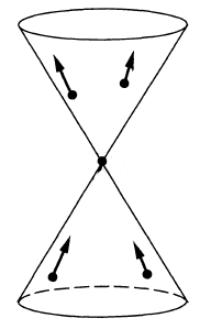
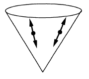
The intuitive idea is that these operators span a Hilbert space of quantum states from a vacuum state characterized by the condition
hence (if we think of as acting by “removing a quantum in mode ”) by the condition that it contains no quanta. So the normal ordered Wick polynomials represent the quantum observables with vanishing vacuum expectation value. In quantum field theory they model scattering processes where quanta enter a reaction process (the modes corresponding to the “annihilation” operators ) and other particles come out of the reaction (the modes corresponding to the “creation” operators ).
The product of two Wick polynomials, computed in the ambient operator algebra and then re-expressed as a Wick polynomial, is given by computing the relevant sequence of commutators by Wick's lemma, for example
where is the value of the canonical commutator.
The associative algebra thus obtained is hence called the algebra of normal ordered operators or Wick polynomial algebra or just Wick algebra.
This plays a central role in perturbative quantum field theory, where the quantization of quantum observables of free fields is traditionally defined as the corresponding Wick algebra.
But the Wick algebra in quantum field theory may also be understood more systematically from first principles of quantization. It turns out that it is Moyal deformation quantization of the canonical Poisson bracket on the covariant phase space of the free field, which is the Peierls bracket modified to an almost Kähler structure by the 2-point function of a quasi-free Hadamard state (Dito 90, Dütsch-Fredenhagen 01).
In free field theory with Green hyperbolic equations of motion, the analog of the star product tensor (this equation)
is the Wightman propagator according to this equation
Understood in this form the construction directly generalizes to quantum field theory on curved spacetimes (Brunetti-Fredenhagen 95, Brunetti-Fredenhagen 00, Hollands-Wald 01).
Finally, the shift by the quasi-free Hadamard state, which is the very source of the “normal ordering”, was understood as an example of the almost-Kähler version of the quantization recipe of Fedosov deformation quantization (Collini 16). For more on this see at locally covariant perturbative quantum field theory.
Definition
Traditionally the Wick algebra is regarded as an operator algebra acting on a Fock space. However, it is useful to realize the Wick algebra directly as an associative algebra structure on the space of microcausal polynomial observables. This “abstract” Wick algebra (meaning: not represented yet on a Hilbert space) we discuss in
That the abstract Wick algebra indeed has a faithful representation on Fock space is Wick's lemma.
Similarly there is the
The traditional notation for the operator products on the Fock space may be carried across the representation map to the abstract Wick algebra:
The abstract Wick algebra carries a canonical state on a star-algebra, whose 2-point function is just the Wightman propagator that the abstract Wick algebra structure is constructed from. This we discuss in
The only non-trivial part of the proof of the state-property (prop. ) below is positivity. This however is immediate from the representation on the Fock space, observing that under this identification the state is represented by the inner product of the Hilbert space (Dütsch 18, remark 2.20). From the point of view of algebraic quantum field theory, the Hilbert space-structure mainly just serves as a technical tool for establishing this positivity property.
Abstract Wick algebra
The abstract Wick algebra of a free field theory with Green hyperbolic differential equation is directly analogous to the star product-algebra induced by a finite dimensional Kähler vector space (this def.) under the following identification of the Wightman propagator with the Kähler space-structure:
Remark
(Wightman propagator as Kähler vector space-structure)
Let be a free Lagrangian field theory whose Euler-Lagrange equation of motion is a Green hyperbolic differential equation. Then the corresponding Wightman propagator is analogous to the rank-2 tensor on a Kähler vector space as follows:
(Fredenhagen-Rejzner 15, section 3.6, Collini 16, table 2.1)
Definition
(microcausal polynomial observables) Let be field bundle which is a vector bundle. An off-shell polynomial observable is a smooth function
on the on-shell space of sections of the field bundle (space of field histories) which may be expressed as
where
is a compactly supported distribution of k variables on the -fold graded-symmetric external tensor product of vector bundles of the field bundle with itself.
Write
for the subspace of off-shell polynomial observables onside all off-shell observables.
Let moreover be a free Lagrangian field theory whose equations of motion are Green hyperbolic differential equations. Then an on-shell polynomial observable is the restriction of an off-shell polynomial observable along the inclusion of the on-shell space of field histories . Write
for the subspace of all on-shell polynomial observables inside all on-shell observables.
By this prop. restriction yields an isomorphism between polynomial on-shell observables and polynomial off-shell observables modulo the image of the differential operator :
Finally a polynomial observable is a microcausal observable if each coefficient as above has wave front set away from those points where the wave vectors are all in the future cone or all in the past cone. We write
for the subspace of off-shell/on-shell microcausal observables inside all off-shell/on-shell polynomial observables.
Proposition
(Hadamard-Moyal star product on microcausal observables – abstract Wick algebra)
Let a free Lagrangian field theory with Green hyperbolic equations of motion . Write for the causal propagator and let
be a corresponding Wightman propagator (Hadamard 2-point function).
Then the star product induced by
on off-shell microcausal observables (def. ) is well defined in that the wave front sets involved in the products of distributions that appear in expanding out the exponential satisfy Hörmander's criterion.
Hence by the general properties of star products (this prop.) this yields a unital associative algebra structure on the space of formal power series in of off-shell microcausal observables
This is the off-shell Wick algebra corresponding to the choice of Wightman propagator .
Moreover the image of is an ideal with respect to this algebra structure, so that it descends to the on-shell microcausal observables to yield the on-shell Wick algebra
Finally, under complex conjugation these are star algebras in that
(Dito 90, Dütsch-Fredenhagen 00 Dütsch-Fredenhagen 01, Hirshfeld-Henselder 02, see Collini 16, p. 25-26)
Proof
By definition of the Wightman propagator (or else by this prop.), the wave front set of powers of has all cotangent wave vectors on the first variables in the closed future cone at the given base point (which itself is on the light cone)
and hence all those on the second variables in the closed past cone.
The first variables are integrated against those of and the second against . By definition of microcausal observables (def. ), the wave front sets of and are disjoint from the subsets where all components are in the closed future cone or all components are in the closed past cone. Therefore the relevant sum of of the wave front covectors never vanishes and hence Hörmander's criterion for partial products of distributions of several variables (this prop.) is met and the star product is well defined.
It remains to see that the star product is itself again a microcausal observable. It is clear that it is again a polynomial observable and that it respects the ideal generated by the equations of motion. That it still satisfies the condition on the wave front set follows directly from the fact that the wave front set of a product of distributions is inside the fiberwise sum of elements of the factor wave front sets (this prop., ).
Finally the star algebra-structure follows via remark as in this prop..
Remark
(Wick algebra is formal deformation quantization of Poisson-Peierls algebra of observables)
Let a free Lagrangian field theory with Green hyperbolic equations of motion with causal propagator and let be a corresponding Wightman propagator (Hadamard 2-point function).
Then the Wick algebra from prop. is a formal deformation quantization of the Poisson algebra on the covariant phase space given by the on-shell polynomial observables equipped with the Poisson-Peierls bracket in that for all we have
and
(Dito 90, Dütsch-Fredenhagen 01)
Proof
By prop. this is immediate from the general properties of the star product (this example).
Explicitly, consider, without restriction of generality, and be two linear observables. Then
Now since is skew-symmetric while is symmetric is follows that
The right hand side is the integral kernel-expression for the Poisson-Peierls bracket, as shown in the second line.
Abstract time-ordered product
Definition
(time-ordered product on regular polynomial observables)
Let be a free Lagrangian field theory over a Lorentzian spacetime and with Green-hyperbolic Euler-Lagrange differential equations; write for the induced causal propagator. Let moreover be a compatible Wightman propagator and write for the induced Feynman propagator.
Then the time-ordered product on the space of off-shell regular polynomial observable is the star product induced by the Feynman propagator (via this prop.):
hence
(Notice that this does not descend to the on-shell observables, since the Feynman propagator is not a solution to the homogeneous equations of motion.)
Proposition
(time-ordered product is indeed causally ordered Wick algebra product)
Let be a free Lagrangian field theory over a Lorentzian spacetime and with Green-hyperbolic Euler-Lagrange differential equations; write for the induced causal propagator. Let moreover be a compatible Wightman propagator and write for the induced Feynman propagator.
Then the time-ordered product on regular polynomial observables (def. ) is indeed a time-ordering of the Wick algebra product in that for all pairs of regular polynomial observables
with disjoint spacetime support we have
Here is the causal order relation (“ does not intersect the past cone of ”). Beware that for general pairs of subsets neither nor .
Proof
Recall the following facts:
-
the advanced and retarded propagators by definition are supported in the future cone/past cone, respectively
-
they turn into each other under exchange of their arguments (this cor.):
-
the real part of the Feynman propagator, which by definition is the real part of the Wightman propagator is symmetric (by definition or else by this prop.):
Using this we compute as follows:
Proposition
(time-ordered product on regular polynomial observables isomorphic to pointwise product)
The time-ordered product on regular polynomial observables (def. ) is isomorphic to the pointwise product of observables (this def.) via the linear isomorphism
given by
in that
hence
(Brunetti-Dütsch-Fredenhagen 09, (12)-(13), Fredenhagen-Rejzner 11b, (14))
Proof
Since the Feynman propagator is symmetric (this prop.), the statement is a special case of this prop.).
Remark
(renormalization of time-ordered product)
The time-ordered product on regular polynomial observables from prop. extends to a product on polynomial local observables, then taking values in microcausal observables:
This extension is not unique. A choice of such an extension, satisfying some evident compatibility conditions, is a choice of renormalization scheme for the given perturbative quantum field theory. Every such choice corresponds to a choice of perturbative S-matrix for the theory. This construction is called causal perturbation theory.
Operator product notation
Definition
(notation for operator product and normal-ordered product)
It is traditional to use the following alternative notation for the product structures on microcausal polynomial observables:
-
The Wick algebra-product, hence the star product for the Wightman propagator (def. ), is rewritten as plain juxtaposition:
-
The pointwise product of observables (this def.) is equivalently written as plain juxtaposition enclosed by colons:
-
The time-ordered product, hence the star product for the Feynman propagator (def. ) is equivalently written as plain juxtaposition prefixed by a “”
Under representation of the Wick algebra on a Fock Hilbert space by linear operators the first product become the operator product, while the second becomes the operator poduct applied after suitable re-ordering, called “normal odering” of the factors.
Disregarding the Fock space-representation, which is faithful, we may still refer to these “abstract” products as the “operator product” and the “normal-ordered product”, respectively.
| free field algebra of quantum observables | physics terminology | maths terminology | |
|---|---|---|---|
| 1) | supercommutative product | normal ordered product | pointwise product of functionals |
| 2) | non-commutative product (deformation induced by Poisson bracket) | operator product | star product for Wightman propagator |
| 3) | time-ordered product | star product for Feynman propagator | |
| perturbative expansion of 2) via 1) | Wick's lemma 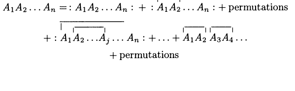 | Moyal product for Wightman propagator | |
| perturbative expansion of 3) via 1) | Feynman diagrams 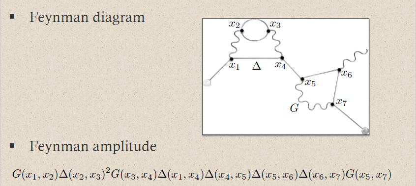 | Moyal product for Feynman propagator |
Hadamard vacuum states
Proposition
(canonical vacuum states on abstract Wick algebra)
Let be a free Lagrangian field theory with Green-hyperbolic Euler-Lagrange equations of motion; and let be a compatible Wightman propagator.
For
any on-shell field history (i.e. solving the equations of motion), consider the function from the Wick algebra to formal power series in with coefficients in the complex numbers which evaluates any microcausal polynomial observable on
Specifically for (which is a solution of the equations of motion by the assumption that defines a free field theory) this is the function
which sends each microcausal polynomial observable to its value on the zero field history, hence to the constant contribution in its polynomial expansion.
The function is
-
linear over ;
-
real, in that for all
-
positive, in that for every there exist a such that
-
normalized, in that
where denotes componet-wise complex conjugation.
This means that is a states on the Wick star-algebra (prop. ). One says that
- is a Hadamard vacuum state;
and generally
- is called a coherent state.
(Dütsch 18, def. 2.12, remark 2.20, def. 5.28, exercise 5.30 and equations (5.178))
Proof
The properties of linearity, reality and normalization are obvious, what requires proof is positivity. This is proven by exhibiting a representation of the Wick algebra on a Fock Hilbert space (this algebra homomorphism is Wick's lemma), with formal powers in suitably taken care of, and showing that under this representation the function is represented, degreewise in , by the inner product of the Hilbert space.
Example
(operator product of two linear observables)
Let
for be two linear microcausal observables represented by distributions which in generalized function-notation are given by
Then their Hadamard-Moyal star product (prop. ) is the sum of their pointwise product with their value
in the Wightman propagator, which is the value of the Hadamard vacuum state from prop.
In the operator product/normal-ordered product-notation of def. this reads
Example
Let a free Lagrangian field theory with Green hyperbolic equations of motion and with Wightman propagator .
Then for
two linear microcausal observables, the Hadamard-Moyal star product (def. ) of their exponentials exhibits the Weyl relations:
where on the right we have the exponential of the value of the Hadamard vacuum state (prop. ) as in example .
(e.g. Dütsch 18, exercise 2.3)
Example
(Wightman propagator is 2-point function in the Hadamard vacuum state)
Let be a free Lagrangian field theory with Green-hyperbolic Euler-Lagrange equations of motion; and let be a compatible Wightman propagator.
With respect to the induced Hadamard vacuum state from prop. , the Wightman propagator itself is the 2-point function, namely the distributional vacuum expectation value of the operator product of two field observables:
Equivalently in the operator product-notation of def. this reads:
Similarly:
Example
(Feynman propagator is time-ordered 2-point function in the Hadamard vacuum state)
Let be a free Lagrangian field theory with Green-hyperbolic Euler-Lagrange equations of motion; and let be a compatible Wightman propagator with induced Feynman propagator .
With respect to the induced Hadamard vacuum state from prop. , the Feynman propagator itself is the time-ordered 2-point function, namely the distributional vacuum expectation value of the time-ordered product (def. ) of two field observables:
Equivalently in the operator product-notation of def. this reads:
propagators (i.e. integral kernels of Green functions)
for the wave operator and Klein-Gordon operator
on a globally hyperbolic spacetime such as Minkowski spacetime:
Related concepts
References
The construction goes back to
- Gian-Carlo Wick, The evaluation of the collision matrix, Phys. Rev. 80, 268-272 (1950)
Its realization as the Moyal deformation quantization of the Peierls bracket shifted by a quasi-free Hadamard state is due to
- Joseph Dito, Star-product approach to quantum field theory: The free scalar field. Letters in Mathematical Physics, 20(2):125–134, 1990 (spire)
further amplified in
-
Michael Dütsch, Klaus Fredenhagen, section 5.1 of Algebraic Quantum Field Theory, Perturbation Theory, and the Loop Expansion, Commun.Math.Phys. 219 (2001) 5-30 (arXiv:hep-th/0001129)
-
Michael Dütsch, Klaus Fredenhagen, Perturbative algebraic field theory, and deformation quantization, in Roberto Longo (ed.), Mathematical Physics in Mathematics and Physics, Quantum and Operator Algebraic Aspects, volume 30 of Fields Institute Communications, pages 151–160. American Mathematical Society, 2001 (arXiv:hep-th/0101079)
-
A. C. Hirshfeld, P. Henselder, Star Products and Perturbative Quantum Field Theory, Annals Phys. 298 (2002) 382-393 (arXiv:hep-th/0208194)
-
Giovanni Collini, Fedosov Quantization and Perturbative Quantum Field Theory (arXiv:1603.09626)
and the generalization to quantum field theory on curved spacetime is discussed in
-
Romeo Brunetti, Klaus Fredenhagen, M. Köhler, The microlocal spectrum condition and Wick polynomials on curved spacetimes, Commun. Math. Phys. 180, 633-652, 1996 (arXiv:gr-qc/9510056)
-
Romeo Brunetti, Klaus Fredenhagen, Microlocal Analysis and Interacting Quantum Field Theories: Renormalization on Physical Backgrounds, Commun. Math. Phys. 208 : 623-661, 2000 (math-ph/9903028)
-
Stefan Hollands, Robert Wald, Local Wick Polynomials and Time Ordered Products of Quantum Fields in Curved Spacetime, Commun. Math. Phys. 223:289-326, 2001 (arXiv:gr-qc/0103074)
Review is in
- Michael Dütsch, section 2.1 of From classical field theory to perturbative quantum field theory, 2018
Last revised on June 20, 2024 at 19:49:28. See the history of this page for a list of all contributions to it.