nLab Feynman diagram

Idea

General

For $\mu_S$ a Gaussian probability measure and $\exp(-I)\mu_S$ a perturbation with $I$ polynomial at least of degree 3, there is a combinatorial expression for the moments/expectation values of $\exp(-I)\mu_S$ as a sum over certain graphs whose $k$-ary vertices are labeled by the monomials of degree $k$ in $I$. (This is such that for $I = 0$ it reduces to Wick's lemma.)

These graphs are called Feynman diagrams.

In perturbative quantum field theory

Feynman graphs play a central role in perturbative quantum field theory, where $\exp(I)\mu_S$ plays the role of an action functional on a space of fields, $\mu_S$ is the exponentiated kinetic action and hence the measure for free fields, while $\exp(I)$ is the interaction part of the action functional: the order-$k$ monomials in $I$ encode an interaction of $k$ fields. In this context the corresponding Feynman diagrams are traditionally thought of as depicting interaction processes of quanta of these fields, with propagation along the edges and interaction at the vertices. But this interpretation has its limits, which is partly reflected in speaking of “virtual particles”. A precise interpretation is given by worldline formalism.

Details

For finitely many degrees of freedoms

We discuss Feynman diagrams for a single real scalar field on a discrete space of $k\in \mathbb{N}$ points. This contains in it already all the aspects of real Feynman diagrams in perturbative quantum field theory and in this context everything is easily well-defined. The generalization to more field components is immediate and simply obtained by thinking of all “$\phi$” in the following as taking values in some appropriate representation space and all products of $\phi$s as given by suitable intertwiners and inner products, otherwise the form of the formulas remains the same. Similarly, in generalization to continuous space (non-finitely many degrees of freedom) all the diagrammatics remains the same, the only issue now is to make sense (namely via renormalization) of the numerical value that is assigned to any one Feynman diagram.

So a field $\phi$ here is a map $[k]\to \mathbb{R}$ from the $k$-element finite set to the real numbers, and hence the space of all field configurations is $\mathbb{R}^k$.

Fix then a $k \times k$ real-valued matrix $A \coloneqq (A_{x y}) \in Mat_{k\times k}(\mathbb{R})$ of non-vanishing determinant $det A \neq 0$.

For standard applications this $A$ is a discretized version of the Laplacian and then the expression

$$S_{kin} = E_{kin} \coloneqq \tfrac{1}{2}\sum_{x,y = 1}^k \phi_x A_{x y} \phi_y$$

is the kinetic energy and kinetic action of the field configuration $\phi$. More concretely, think of the set of $k$ space points as being a discretization of a circle and write $(\phi_p)$ for the corresponding (discrete) Fourier transform of $(\phi_x)$. Then the kinetic term of the free scalar field on this space is given by $A$ which is the diagonal matrix in the $p$-basis with

$$A_{p,p} = p^2 - m^2 \,,$$

where $m$ is a constant called the mass of the field $\phi$.

A sum over all values of $\phi$ is the finite (and hence well-defined) analog of a path integral. The Gaussian integral of $A$ is called the partition function:

$$\begin{aligned} Z_0 & \coloneqq \int \exp(- S_{kin}(\phi)) \,D\phi \\ & \coloneqq \int_{\mathbb{R}^k} \, \exp(- \tfrac{1}{2}\sum_{x,y = 1}^k \phi_{x} A_{x,y} \phi_y ) \; d\phi_{1} \cdots d\phi_{k} \\ & = (2\pi)^{k/2} (det A)^{-1/2} \end{aligned}$$

An n-point function $\langle \phi_{x_1} \phi_{x_2} \cdots \phi_{x_n}\rangle$ is an $n$th moment of this Gaussian distribution:

$$\begin{aligned} \langle \phi_{x_1} \phi_{x_2} \cdots \phi_{x_n}\rangle & \coloneqq \frac{1}{Z_0} \int \left( \exp(-S_{kin}(\phi)) \phi_{x_1}\phi_{x_2}\cdots \phi_{x_n} \right) D \phi \\ & \coloneqq \frac{1}{Z_0} \int_{\mathbb{R}^k} \left( \exp(-\tfrac{1}{2} \phi_x A_{x,y}\phi_y) \, \phi_{x_1}\phi_{x_2} \cdots\phi_{x_n} \right) d\phi_1 \cdots d\phi_k \end{aligned}$$

In order to compute these conveniently, pass to the generating function obtained by adding a source variable $J = (J_x)$:

$$\begin{aligned} Z(J) & \coloneqq \int( \exp(- S_{kin}(\phi) + J \cdot\phi) ) D\phi \\ & \coloneqq \int_{\mathbb{R}^k} \exp(- \tfrac{1}{2}\sum_{x = 1}^k \phi_{x} A_{x,y} \phi_y + \sum_{x = 1}^k J_x \phi_x ) \; d\phi_{1} \cdots d\phi_{k} \\ & = Z_0 \exp(\tfrac{1}{2} \sum_{x = 1}^k J_x A^{-1}_{x,y} J_y) \end{aligned} \,,$$

where $A^{-1} = (A^{-1}_{x,y})$ is the inverse matrix of $A$, which appears by computing the new integral here again as a Gaussian integral after completing the square in the exponent.

In applications to field theory this $A^{-1}$ is called the Feynman propagator. In the standard example where $A$ is the kinetic term of the free field of mass $m$ then in Fourier-transformed components $A^{-1}$ is diagonal with components

$$A^{-1}_{p,p} = \frac{1}{p^2 - m^2} \,.$$

This means, incidentally. that in the non-finite case of interest in physics, $A$ is not actually naively invertible after all, as $p^2 = m^2$ on the mass shell. In this case one has to replace the naive $A^{-1}$ with its zeta-function regularized version.

The way this works is insightful even when the naive $A^{-1}$ does exist. Notice that using “Schwinger parameterization” the propagator is equivalently rewritten as a Mellin transform integral:

$$A^{-1}_{p,p} = \int_0^\infty \exp(- \tau A_{p,p}) d\tau \,.$$

Again in the example of the standard scalar field kinetic term expressed in Fourier diagonalization $A_{p,p}= p^2 - m^2$ then with $X \colon [0,\tau] \to \mathbb{R}$ a parameterization of the straight line with slope $p$, the exponent is equivalently

$$\begin{aligned} \tau A_{p,p} & = \tau (p^2 - m^2) \\ & = \int_0^\tau (\dot X^2 - m^2) \end{aligned} \,.$$

This now happens to be the standard action functional (Polyakov action) for a sigma model describing the propagation of a particle along its worldline. This means that the propagator of the scalar field may be thought of as coming from the path integral of a scalar particle along its worldline. This perspective is called the “worldline formalism”, it is a formalization of second quantization, expressing the dynamics of fields in terms of that of their particle “quanta” running along worldlines of the form of the corresponding Feynman diagrams (to which we finally come in a moment).

Back to the computation of the $n$-point function. By construction, it is now equally expressed by partial derivatives of the generating function with respect to the source variable $J$ and evaluated at $J = 0$, and this in turn is a combinatorial expression just in products of the propagator:

$$\begin{aligned} \langle \phi_{x_1} \cdots \phi_{x_n} \rangle &= \frac{1}{Z_0} \left( \frac{\partial}{\partial J_{x_1}} \cdots \frac{\partial}{\partial J_{x_n}} Z(J) \right)_{\vert J = 0} \\ & = \left( \frac{\partial}{\partial J_{x_1}} \cdots \frac{\partial}{\partial J_{x_n}} \exp(\tfrac{1}{2} \sum_{x = 1}^k J_{x} A^{-1}_{x y} J_y) \right)_{\vert J = 0} \\ & = \underset{pairings}{\sum} A^{-1}_{x_{j_1} x_{j_2}} \cdot A^{-1}_{x_{j_3} x_{j_4}} \cdots A^{-1}_{x_{j_{n-1}}x_{j_n}} \end{aligned} \,.$$

Here the last equality – known as Wick's theorem – comes from simple inspection: take the derivatives inside the exponential series and observe that then the only summands non-vanishing at $J = 0$ appears for even $n$ and are those where all derivatives hit the monomial $\left(\tfrac{1}{2} \sum_{x = 1}^k J_{x} A^{-1}_{x y} J_y\right)^{n/2}$.

Thinking of $A^{-1}_{x y}$ here as labeling an edge (a “worldline”) from vertex $x$ to vertex $y$ This is the source of all Feynman digrammatics.

Now consider a polynomial $V(\phi)$ of degree $\geq 3$. In applications to field theory this represents the potential energy or (self)interaction of the field configuration. The difference of the kinetic energy and the potential energy is called the (here: “Wick rotated”/“Euclidean”) action

$$\begin{aligned} S & = S_{kin} + S_{int} \\ & = \tfrac{1}{2} \sum_{x,y = 1}^k \phi_x A_{x y} \phi_y - g V(\phi) \end{aligned} \,.$$

The prefactor $g$ is called the coupling constant.

Putting everything together, the integral over the full action may be expressed as a power series in the coupling constant $g$ of the moments with respect to the kinetic action of the powers of the interaction term:

$$\begin{aligned} Z(g) & = \frac{1}{Z_0}\int \exp(- S(\phi)) \, D\phi \\ & \coloneqq \frac{1}{Z_0} \int \left(\exp(-\tfrac{1}{2} \sum_{x,y = 1}^k \phi_x A_{x y} \phi_y + g V(\phi)) \right) \, d\phi_1 \cdots d\phi_k \\ & = \langle \exp(g V(\phi)) \rangle \\ & = 1 + g \langle V(\phi)\rangle + \frac{g^2}{2} \langle V(\phi) ^2\rangle + \cdots \end{aligned}$$

By Wick's theorem stated above, each $\langle V(\phi)^\ell\rangle$ is equivalently expressed as a sum over products of components of the propagator $A^{-1}_{x y}$. Thinking of each such propagator term as an edge produces a diagram, this is the corresponding Feynman diagram.

For instance, for a cubic point interaction

$$V(\phi) = \sum_x \phi_x^3$$

then

$$\begin{aligned} \langle V(\phi)^2 \rangle &\coloneqq \langle (\sum_{x= 1}^k \phi_x^3)^2 \rangle \\ & = \sum_{x_1, x_2 = 1}^k \langle \phi_{x_1}\phi_{x_1} \phi_{x_1}\phi_{x_2}\phi_{x_2}\phi_{x_2}\rangle \\ & = prefactor \; \sum_{x_1,x_2 = 1}^k \underset{dumbbell\, diagram}{\underbrace{A^{-1}_{x_1 x_1} A^{-1}_{x_1 x_2} A^{-1}_{x_2 x_2}}} + prefactor \; \sum_{x_1, x_2 = 1}^k \underset{theta\, diagram}{\underbrace{A^{-1}_{x_1 x_2} A^{-1}_{x_1 x_2} A^{-1}_{x_1 x_2}}} \end{aligned}$$

Here the first summand corresponds to the “dumbbell” Feynman diagram of the form

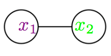
and the second summand corresponds to the “theta” Feynman diagram of the form

.

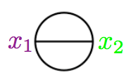In perturbative quantum field theory

For details see at

• S-matrix the section Feynman perturbation series

$\,$

	free field algebra of quantum observables	physics terminology	maths terminology
1)	supercommutative product	$\phantom{AA} :A_1 A_2:$ normal ordered product	$\phantom{AA} A_1 \cdot A_2$ pointwise product of functionals
2)	non-commutative product (deformation induced by Poisson bracket)	$\phantom{AA} A_1 A_2$ operator product	$\phantom{AA} A_1 \star_H A_2$ star product for Wightman propagator
3)		$\phantom{AA} T(A_1 A_2)$ time-ordered product	$\phantom{AA} A_1 \star_F A_2$ star product for Feynman propagator
	perturbative expansion of 2) via 1)	Wick's lemma	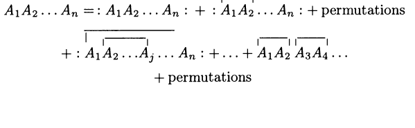Moyal product for Wightman propagator $\Delta_H$ $\begin{aligned} & A_1 \star_H A_2 = \\ & ((-)\cdot (-)) \circ \exp \left( \hbar \int (\Delta_H)^{ab}(x,y) \frac{\delta}{\delta \mathbf{\Phi}^a(x)} \otimes \frac{\delta}{\delta \mathbf{\Phi}^b(y)} \right)(A_1 \otimes A_2) \end{aligned}$
	perturbative expansion of 3) via 1)	Feynman diagrams	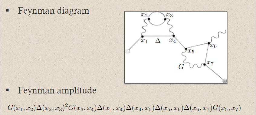Moyal product for Feynman propagator $\Delta_F$ $\begin{aligned} & A_1 \star_F A_2 = \\ & ((-)\cdot (-)) \circ \exp \left( \hbar \int (\Delta_F)^{ab}(x,y) \frac{\delta}{\delta \mathbf{\Phi}^a(x)} \otimes \frac{\delta}{\delta \mathbf{\Phi}^b(y)} \right)(A_1 \otimes A_2) \end{aligned}$

$\,$

Example

(Feynman amplitudes in causal perturbation theory – example of QED)

In perturbative quantum field theory, Feynman diagrams are labeled multigraphs that encode products of Feynman propagators, called Feynman amplitudes (this prop.) which in turn contribute to probability amplitudes for physical scattering processes – scattering amplitudes:

The Feynman amplitudes are the summands in the Feynman perturbation series-expansion of the scattering matrix

$$\mathcal{S} \left( S_{int} \right) = \underset{k \in \mathbb{N}}{\sum} \frac{1}{k!} \frac{1}{(i \hbar)^k} T( \underset{k \, \text{factors}}{\underbrace{S_{int}, \cdots , S_{int}}} )$$

of a given interaction Lagrangian density $L_{int}$.

The Feynman amplitudes are the summands in an expansion of the time-ordered products $T(\cdots)$ of the interaction with itself, which, away from coincident vertices, is given by the star product of the Feynman propagator $\Delta_F$ (this prop.), via the exponential contraction

$$T(S_{int}, S_{int}) \;=\; prod \circ \exp \left( \hbar \int \Delta_{F}^{a b}(x,y) \frac{\delta}{\delta \mathbf{\Phi}^a(x)} \otimes \frac{\delta}{\delta \mathbf{\Phi}(y)} \right) ( S_{int} \otimes S_{int} ) \,.$$

Each edge in a Feynman diagram corresponds to a factor of a Feynman propagator in $T( \underset{k \, \text{factors}}{\underbrace{S_{int} \cdots S_{int}}} )$, being a distribution of two variables; and each vertex corresponds to a factor of the interaction Lagrangian density at $x_i$.

For example quantum electrodynamics in Gaussian-averaged Lorenz gauge involves (via this example):

1. the Dirac field modelling the electron, with Feynman propagator called the electron propagator (this def.), here to be denoted

   $$\Delta \phantom{AAAA} \text{electron propagator}$$

2. the electromagnetic field modelling the photon, with Feynman propagator called the photon propagator (this prop.), here to be denoted

   $$G \phantom{AAAA} \text{photon propagator}$$

3. the electron-photon interaction

   $$L_{int} \;=\; \underset{ \text{interaction} }{ \underbrace{ i g (\gamma^\mu)^\alpha{}_\beta } } \, \underset{ { \text{incoming} \atop \text{electron} } \atop \text{field} }{\underbrace{\overline{\psi_\alpha}}} \; \underset{ { \, \atop \text{photon} } \atop \text{field} }{\underbrace{a_\mu}} \; \underset{ {\text{outgoing} \atop \text{electron} } \atop \text{field} }{\underbrace{\psi^\beta}}$$

The Feynman diagram for the electron-photon interaction alone is

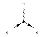
where the solid lines correspond to the electron, and the wiggly line to the photon. The corresponding product of distributions is (written in generalized function-notation)

$$\underset{ \text{loop order} }{ \underbrace{ \hbar^{3/2-1} } } \underset{ \text{electron-photon} \atop \text{interaction} }{ \underbrace{ i g (\gamma^\mu)^\alpha{}_\beta } } \,. \, \underset{ {\text{incoming} \atop \text{electron}} \atop \text{propagator} }{ \underbrace{ \overline{\Delta(-,x)}_{-, \alpha} } } \underset{ { \, \atop \text{photon} } \atop \text{propagator} }{ \underbrace{ G(x,-)_{\mu,-} } } \underset{ { \text{outgoing} \atop \text{electron} } \atop \text{propagator} }{ \underbrace{ \Delta(x,-)^{\beta, -} } }$$

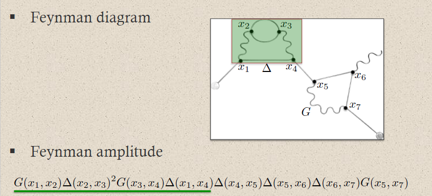
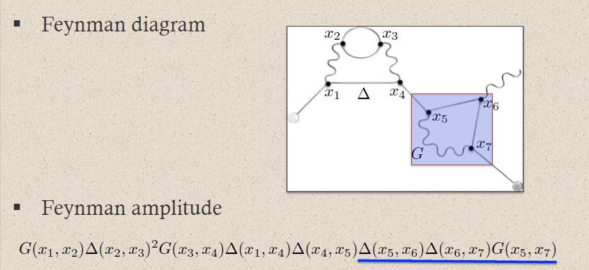
Hence a typical Feynman diagram in the QED Feynman perturbation series induced by this electron-photon interaction looks as follows:

where on the bottom the corresponding Feynman amplitude product of distributions is shown; now notationally suppressing the contraction of the internal indices and all prefactors.

For instance the two solid edges between the vertices $x_2$ and $x_3$ correspond to the two factors of $\Delta(x_2,x_2)$:

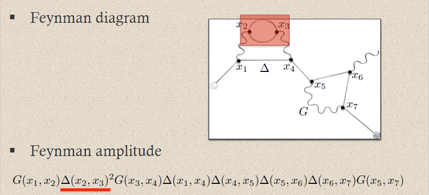
This way each sub-graph encodes its corresponding subset of factors in the Feynman amplitude:

graphics grabbed from Brouder 10

A priori this product of distributions is defined away from coincident vertices: $x_i \neq x_j$. The definition at coincident vertices $x_i = x_j$ requires a choice of extension of distributions to the diagonal locus. This choice is the ("re-")normalization of the Feynman amplitude.

Related concepts

• vacuum diagram

• perturbative quantum field theory

• S-matrix, perturbation series

• causal perturbation theory

• path integral quantization

• scattering amplitude, string scattering amplitude

• Feynman propagator

• worldline formalism

• Schwinger-Dyson equation

• tadpole

• loop order

• radiative correction

• graph complex, formality of the little n-disk operad

References

General

Traditional review:

• Radovan Dermisek, Path integral for interacting field (pdf)

• Stefan Weinzierl, Introduction to Feynman Integrals [arXiv:1005.1855]

• Stefan Weinzierl, Feynman Integrals, UNITEXT for Physics, Springer (2022) [arXiv:2201.03593, doi:10.1007/978-3-030-99558-4] (816 pages)

See also

• Alain Connes, Matilde Marcolli, section 3 of Noncommutative Geometry, Quantum Fields and Motives

• Wikipedia, Feynman diagram

• F. T. Brandt, J. Frenkel, D. G. C. McKeon, Feynman diagrams in terms of on-shell propagators [arXiv:2206.14860]

• Zhi-Feng Liu, Yan-Qing Ma, Determining Feynman Integrals with Only Input from Linear Algebra, Physical Review Letters, Volume 129, Issue 22, 23 November 2022 (doi:10.1103/PhysRevLett.129.222001, arXiv:2201.11637)

Discussion via D-modules:

• Johannes Henn, Elizabeth Pratt, Anna-Laura Sattelberger, Simone Zoia, $D$-Module Techniques for Solving Differential Equations in the Context of Feynman Integrals [arXiv:2303.11105]

In causal perturbation theory

Discussion of Feynman diagrams in the rigorous formulation of causal perturbation theory and perturbative AQFT is due to

• Kai Keller, chapter IV of Dimensional Regularization in Position Space and a Forest Formula for Regularized Epstein-Glaser Renormalization, PhD thesis (arXxiv:1006.2148)

parts of which also appears as

• Michael Dütsch, Klaus Fredenhagen, Kai Keller, Katarzyna Rejzner, Dimensional Regularization in Position Space, and a Forest Formula for Epstein-Glaser Renormalization, J. Math. Phy.

  55(12), 122303 (2014) (arXiv:1311.5424)

An exposition of this is in

• Christian Brouder, Multiplication of distributions, 2010 (pdf)

Relation to the Hopf algebra structure on Feynman diagrams due to Kreimer 97 is discussed in

• Jose Gracia-Bondia, S. Lazzarini, Connes-Kreimer-Epstein-Glaser Renormalization (arXiv:hep-th/0006106)

Relation to periods (in the sense here) is discussed in

• Kasia Rejzner, Renormalization and periods in perturbative Algebraic Quantum Field Theory (arXiv:1603.02748)

See also

• Eli Hawkins, Kasia Rejzner, section 5.2 of The Star Product in Interacting Quantum Field Theory (arXiv:1612.09157)

Review is in

• Katarzyna Rejzner, section 6.5.2 of Perturbative Algebraic Quantum Field Theory, Mathematical Physics Studies, Springer 2016 (pdf)

In terms of motivic structures

In terms of motives (see also motives in physics)

• Spencer Bloch, Helene Esnault, Dirk Kreimer, On motives associated to graph polynomials, (pdf)

• Spencer Bloch, Pierre Vanhove, The elliptic dilogarithm for the sunset graph, IHES preprint P-13-24, pdf

In homological BV-quantization

A clean derivation of the Feynman rules for finite-dimensional spaces of fields in terms of quantization by passing to cochain cohomology of BV-complexes (see at BV-formalism – Homological quantization) is in

• Owen Gwilliam, Theo Johnson-Freyd, How to derive Feynman diagrams for finite-dimensional integrals directly from the BV formalism (2011) (arXiv:1202.1554)

with a review in the broader context of factorization algebras of observables in section 2.3 of

• Owen Gwilliam, Factorization algebras and free field theories (pdf)

As string diagrams (morphisms in monoidal categories)

It has been observed that Feynman diagrams, notably in gauge theory, are in particular string diagrams (in the sense of category theory, not here in any sense of string theory!) in the given category of representations: the edges are labelled by particle species, hence by Wigner classification by irreps, and the vertices are labeled by representation homomorphisms (“intertwiners”) which, indeed, label the interaction of particles in the Feynman diagram.

A review of this formulation is in

• John Baez, Aaron Lauda, A Prehistory of n-Categorical Physics, Deep beauty, 13-128, Cambridge Univ. Press, Cambridge, 2011 (arXiv:0908.2469)

Moreover, one may think of string diagrams in monoidal categories as providing categorical semantics for proof nets (see there for more) in multiplicative linear logic. Under this identification then Feynman diagrams have a relation to proof nets. Something like this is discussed in

• Richard Blute, Prakash Panangaden, Proof nets as formal Feynman diagrams (pdf)