nLab A first idea of quantum field theory -- Free quantum fields

Free quantum fields

In this chapter we discuss the following topics:

• Wick algebra

• Time-ordered product

• Operator product notation

• Hadamard vacuum state

• Free quantum BV-differential

• Schwinger-Dyson equation

$\,$

In the previous chapter we discussed quantization of linear phase spaces, which turns the algebra of observables into a noncommutative algebra of quantum observables. Here we apply this to the covariant phase spaces of gauge fixed free Lagrangian field theories (as discussed in the chapter Gauge fixing), obtaining genuine quantum field theory for free fields.

For this purpose we first need to find a sub-algebra of all observables which is large enough to contain all local observables (such as the phi^n interaction, example below, and the electron-photon interaction, example below) but small enough for the star product deformation quantization to meet Hörmander's criterion for absence of UV-divergences (remark ). This does exist (example below): It is called the algebra of microcausal polynomial observables (def. below).

types of observables in perturbative quantum field theory:

$$\array{ && \text{local} \\ && & \searrow \\ \text{field} &\longrightarrow& \text{linear} &\longrightarrow& \text{microcausal} &\longrightarrow& \text{polynomial} &\longrightarrow& \text{general} \\ && & \nearrow \\ && \text{regular} }$$

While the star product of the causal propagator still violates Hörmander's criterion for absence of UV-divergences on microcausal polynomial observables, we have seen in the previous chapter that qantization freedom allows to shift this Poisson tensor by a symmetric contribution. By prop. such a shift is provided by passage from the causal propagator to the Wightman propagator, and by prop. this reduces the wave front set and hence the UV-singularities “by half”.

This way the deformation quantization of the Peierls-Poisson bracket exists on microcausal polynomial observables as the star product algebra induced by the Wightman propagator. The resulting non-commutative algebra of observables is called the Wick algebra (prop. below). Its algebra structure may be expressed in terms of a commutative “normal-ordered product” (def. below) and the vacuum expectation values of field observables in a canonically induced vacuum state (prop. below).

The analogous star product induced by the Feynman propagator (def. below) acts by first causal ordering its arguments and then multiplying them with the Wick algebra product (prop. below) and hence is called the time-ordered product (def. below). This is the key structure in the discussion of interacting field theory discussed in the next chapter Interacting quantum fields. Here we consider this on regular polynomial observables only, hence for averages of field observables that evaluate at distinct spacetime points. The extension of the time-ordered product to local observables is possible, but requires making choices: This is called renormalization, which we turn to in the chapter Renormalization below.

	free field algebra of quantum observables	physics terminology	maths terminology
1)	supercommutative product	$\phantom{AA} :A_1 A_2:$ normal ordered product	$\phantom{AA} A_1 \cdot A_2$ pointwise product of functionals
2)	non-commutative product (deformation induced by Poisson bracket)	$\phantom{AA} A_1 A_2$ operator product	$\phantom{AA} A_1 \star_H A_2$ star product for Wightman propagator
3)		$\phantom{AA} T(A_1 A_2)$ time-ordered product	$\phantom{AA} A_1 \star_F A_2$ star product for Feynman propagator
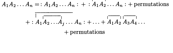
	perturbative expansion of 2) via 1)	Wick's lemma	Moyal product for Wightman propagator $\Delta_H$ $\begin{aligned} & A_1 \star_H A_2 = \\ & ((-)\cdot (-)) \circ \exp \left( \hbar \int (\Delta_H)^{ab}(x,y) \frac{\delta}{\delta \mathbf{\Phi}^a(x)} \otimes \frac{\delta}{\delta \mathbf{\Phi}^b(y)} \right)(A_1 \otimes A_2) \end{aligned}$
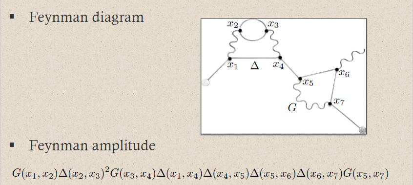
	perturbative expansion of 3) via 1)	Feynman diagrams	Moyal product for Feynman propagator $\Delta_F$ $\begin{aligned} & A_1 \star_F A_2 = \\ & ((-)\cdot (-)) \circ \exp \left( \hbar \int (\Delta_F)^{ab}(x,y) \frac{\delta}{\delta \mathbf{\Phi}^a(x)} \otimes \frac{\delta}{\delta \mathbf{\Phi}^b(y)} \right)(A_1 \otimes A_2) \end{aligned}$

While the Wick algebra with its vacuum state provides a quantization of the algebra of observables of free gauge fixed Lagrangian field theories, the possible existence of infinitesimal gauge symmetries implies that the physically relevant observables are just the gauge invariant on-shell ones, exhibited by the cochain cohomology of the BV-BRST differential $\{-S' + S'_{BRST}, (-)\}$. Hence to complete quantization of gauge theories, the BV-BRST differential needs to be lifted to the noncommutative algebra of quantum observables – this is called BV-BRST quantization.

To do so, we may regard the gauge fixed BRST-action functional $S'_{BRST}$ as an interaction term, to be dealt with later via scattering theory, and hence consider quantization of just the free BV-differential $\{-S',(-)\}$. One finds that this is equal to its time-ordered version $\{-S',(-)\}_{\mathcal{T}}$ (prop. below) plus a quantum correction, called the BV-operator (def. below) or BV-Laplacian (prop. below).

Applied to observables this relation is the Schwinger-Dyson equation (prop. below), which expresses the quantum-correction to the equations of motion of the free gauge field Lagrangian field theory as seen by time-ordered products of observables (example below.)

After introducing field-interactions via scattering theory in the next chapter the quantum correction to the BV-differential by the BV-operator becomes the “quantum master equation” and the Schwinger-Dyson equation becomes the “master Ward identity”. When choosing renormalization these identities become conditions to be satisfied by renormalization choices in order for the interacting quantum BV-BRST differential, and hence for gauge invariant quantum observables, to be well defined in perturbative quantum field theory of gauge theories. This we discuss below in Renormalization.

$\,$

Wick algebra

The abstract Wick algebra of a free field theory with Green hyperbolic differential equation is directly analogous to the star product-algebra induced by a finite dimensional Kähler vector space (def. ) under the following identification of the Wightman propagator with the Kähler space-structure:

Remark

(Wightman propagator as Kähler vector space-structure)

Let $(E,\mathbf{L})$ be a free Lagrangian field theory whose Euler-Lagrange equation of motion is a Green hyperbolic differential equation. Then the corresponding Wightman propagator is analogous to the rank-2 tensor on a Kähler vector space as follows:

covariant phase space of free Green hyperbolic Lagrangian field theory	finite dimensional Kähler vector space
space of field histories $\Gamma_\Sigma(E)$	$\mathbb{R}^{2n}$
symplectic form $\tau_{\Sigma_p} \Omega_{BFV}$	Kähler form $\omega$
causal propagator $\Delta$	$\omega^{-1}$
Peierls-Poisson bracket $\{A_1,A_2\} = \int \Delta^{a_1 a_2}(x_1,x_2) \frac{\delta A_1}{\delta \mathbf{\Phi}^{a_1}(x_1)} \frac{\delta A_2}{\delta \mathbf{\Phi}^{a_2}(x_2)} dvol_\Sigma(x)$	Poisson bracket
Wightman propagator $\Delta_H = \tfrac{i}{2} \Delta + H$	Hermitian form $\pi = \tfrac{i}{2}\omega^{-1} + \tfrac{1}{2}g^{-1}$

(Fredenhagen-Rejzner 15, section 3.6, Collini 16, table 2.1)

Definition

(microcausal polynomial observables)

Let $E \overset{fb}{\to} \Sigma$ be a field bundle which is a vector bundle, over some spacetime $\Sigma$.

A polynomial observable (def. )

$$\begin{aligned} A & = \phantom{+} \alpha^{(0)} \\ & \phantom{=} + \int_{\Sigma} \mathbf{\Phi}^a(x) \alpha^{(1)}_a(x) \, dvol_\Sigma(x) \\ & \phantom{=} + \int_{\Sigma^2} \mathbf{\Phi}^{a_1}(x_1) \cdot \mathbf{\Phi}^{a_2}(x_2) \alpha^{(2)}_{a_1 a_2}(x_1, x_2) \, dvol_\Sigma(x_1) dvol_\Sigma(x_2) \\ & \phantom{=} + \int_{\Sigma^3} \mathbf{\Phi}^{a_1}(x_1) \cdot \mathbf{\Phi}^{a_2}(x_2) \cdot \mathbf{\Phi}^{a_3}(x_3) \alpha^{(3)}_{a_1 a_2 a_3}(x_1,x_2,x_3) \, dvol_\Sigma(x_1) dvol_\Sigma(x_2) dvol_\Sigma(x^3) \\ & \phantom{=} + \cdots \,. \end{aligned}$$

is called microcausal if each distributional coefficient

$$\alpha^{(k)} \;\in\; \Gamma'_{\Sigma^k}(E^{\boxtimes^k})$$

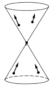
as above has wave front set (def. ) not containing those elements $(x_1, \cdots x_k, k_1, \cdots k_k)$ where the $k$ wave vectors are all in the closed future cone or all in the closed past cone (def. ).

We write

$$\array{ PolyObs(E)_{mc} &\hookrightarrow& PolyObs(E) \\ PolyObs(E,\mathbf{L})_{mc} \simeq PolyObs(E)_{mc}/im(P) &\hookrightarrow& PolyObs(E,\mathbf{L}) }$$

for the subspace of off-shell/on-shell microcausal polynomial observables inside all off-shell/on-shell polynomial observables.

The important point is that microcausal polynomial observables still contain all regular polynomial observables but also all polynomial local observables:

Example

(regular polynomial observables are microcausal)

Every regular polynomial observable (def. ) is microcausal (def. ).

Proof

By definition of regular polynomial observables, their coefficients are non-singular distributions and because the wave front set of non-singular distributions is empty (example )

Example

(polynomial local observables are microcausal)

Every polynomial local observable (def. ) is a microcausal polynomial observable (def. ).

Proof

For notational convenience, consider the case of the scalar field with $k = 2$; the general case is directly analogous. Then the local observable coming from $\phi^2$ (a phi^n interaction-term), has, regarded as a polynomial observable, the delta distribution $\delta(x_1-x_2)$ as coefficient in degree 2:

$$\begin{aligned} A(\Phi) & = \underset{\Sigma}{\int} g(x) (\Phi(x))^2 \,dvol_\Sigma(x) \\ & = \underset{\Sigma \times \Sigma}{\int} \underset{ = \alpha^{(2)}}{ \underbrace{ g(x_1) \delta(x_1 - x_2) }} \, \Phi(x_1) \Phi(x_2) \, dvol_\Sigma(x_1) \, dvol_\Sigma(x_2) \end{aligned} \,.$$

Now for $(x_1, x_2) \in \Sigma \times \Sigma$ and $\mathbb{R}^{2n} \simeq U \subset X \times X$ a chart around this point, the Fourier transform of distributions of $g \cdot \delta(-,-)$ restricted to this chart is proportional to the Fourier transform $\hat g$ of $g$ evaluated at the sum of the two covectors:

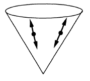
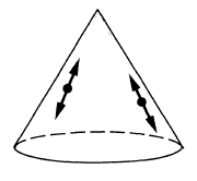
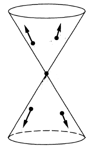
$$\begin{aligned} (k_1, k_2) & \mapsto \underset{\mathbb{R}^{2n}}{\int} g(x_1) \delta(x_1, x_2) e^{i (k_1 \cdot x_1 + k_2 \cdot x_2 )} \, dvol_\Sigma(x_1) \, dvol_\Sigma(x_2) \\ & \propto \hat g(k_1 + k_2) \end{aligned} \,.$$

Since $g$ is a plain bump function, its Fourier transform $\hat g$ is quickly decaying (according to prop. ) along $k_1 + k_2$, as long as $k_1 + k_2 \neq 0$. Only on the cone $k_1 + k_2 = 0$ the Fourier transform is constant, and hence in particular not decaying.

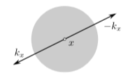
This means that the wave front set consists of the elements of the form $(x, (k, -k))$ with $k \neq 0$. Since $k$ and $-k$ are both in the closed future cone or both in the closed past cone precisely if $k = 0$, this situation is excluded in the wave front set and hence the distribution $g \cdot \delta(-,-)$ is microcausal.

(graphics grabbed from Khavkine-Moretti 14, p. 45)

Proposition

(Hadamard-Moyal star product on microcausal observables – abstract Wick algebra)

Let $(E,\mathbf{L})$ a free Lagrangian field theory with Green hyperbolic equations of motion $P \Phi = 0$. Write $\Delta$ for the causal propagator and let

$$\Delta_H \;=\; \tfrac{i}{2}\Delta + H$$

be a corresponding Wightman propagator (Hadamard 2-point function).

Then the star product induced by $\Delta_H$

$$A \star_H A \;\coloneqq\; prod \circ \exp\left( \int_{X^2} \hbar \Delta_H^{a b}(x_1, x_2) \frac{\delta}{\delta \mathbf{\Phi}^a(x_1)} \otimes \frac{\delta}{\delta \mathbf{\Phi}^b(x_2)} dvol_g \right) (P_1 \otimes P_2)$$

on off-shell microcausal observables $A_1, A_2 \in \mathcal{F}_{mc}$ (def. ) is well defined in that the wave front sets involved in the products of distributions that appear in expanding out the exponential satisfy Hörmander's criterion.

Hence by the general properties of star products (prop. ) this yields a unital associative algebra structure on the space of formal power series in $\hbar$ of off-shell microcausal observables

$$\left( PolyObs(E)_{mc}[ [\hbar] ] \,,\, \star_H \right) \,.$$

This is the off-shell Wick algebra corresponding to the choice of Wightman propagator $H$.

Moreover the image of $P$ is an ideal with respect to this algebra structure, so that it descends to the on-shell microcausal observables to yield the on-shell Wick algebra

$$\left( PolyObs(E,\mathbf{L})_{mc}[ [ \hbar ] ] \,,\, \star_H \right) \,.$$

Finally, under complex conjugation $(-)^\ast$ these are star algebras in that

$$\left( A_1 \star_H A_2 \right)^\ast = A_2^\ast \star_H A_1^\ast \,.$$

(e.g. Collini 16, p. 25-26)

Proof

By prop. the wave front set of $\Delta_H$ has all cotangents on the first variables in the closed future cone (at the given base point, which itself is on the light cone)

and hence all those on the second variables in the closed past cone.

The first variables are integrated against those of $A_1$ and the second against $A_2$. By definition of microcausal observables (def. ), the wave front sets of $A_1$ and $A_2$ are disjoint from the subsets where all components are in the closed future cone or all components are in the closed past cone. Therefore the relevant sum of of the wave front covectors never vanishes and hence Hörmander's criterion (prop. ) for partial products of distributions of several variables (prop. ).

It remains to see that the star product $A_1 \star_H A_2$ is itself again a microcausal observable. It is clear that it is again a polynomial observable and that it respects the ideal generated by the equations of motion. That it still satisfies the condition on the wave front set follows directly from the fact that the wave front set of a product of distributions is inside the fiberwise sum of elements of the factor wave front sets (prop. , prop. ).

Finally the star algebra-structure via complex conjugation follows via remark as in prop. .

Remark

(Wick algebra is formal deformation quantization of Poisson-Peierls algebra of observables)

Let $(E,\mathbf{L})$ a free Lagrangian field theory with Green hyperbolic equations of motion $P \Phi = 0$ with causal propagator $\Delta$ and let $\Delta_H \;=\; \tfrac{i}{2}\Delta + H$ be a corresponding Wightman propagator (Hadamard 2-point function).

Then the Wick algebra $\left( PolyObs(E,\mathbf{L})_{mc}[ [\hbar] ] \,,\, \star_H \right)$ from prop. is a formal deformation quantization of the Poisson algebra on the covariant phase space given by the on-shell polynomial observables equipped with the Poisson-Peierls bracket $\{-,-\} \;\colon\; PolyObs(E,\mathbf{L})_{mc} \otimes PolyObs(E,\mathbf{L})_{mc} \to PolyObs(E,\mathbf{L})_{mc}$ in that for all $A_1, A_2 \in PolyObs(E,\mathbf{L})_{mc}$ we have

$$A_1 \star_H A_2 \;=\; A_1 \cdot A_2 \;mod\; \hbar$$

and

$$A_1 \star_H A_2 - A_2 \star_H a_1 \;=\; i \hbar \{A_1, A_2\} \;mod\; \hbar^2 \,.$$

(Dito 90, Dütsch-Fredenhagen 00, Dütsch-Fredenhagen 01, Hirshfeld-Henselder 02)

Proof

By prop. this is immediate from the general properties of the star product (example ).

Explicitly, consider, without restriction of generality, $A_1 = \int (\alpha_1)_a(x) \mathbf{\Phi}^a(x)\, dvol_\Sigma(x)$ and $A_2 = \int (\alpha_2)_a(x) \mathbf{\Phi}^a(x)\, dvol_\Sigma(x)$ be two linear observables. Then

$$\begin{aligned} & A_1 \star_H A_2 \\ & = \phantom{+} A_1 A_2 \\ & \phantom{=} + \hbar \int \left( \tfrac{i}{2} \Delta^{a_1 a_2}(x_1, x_2) + H^{a_1 a_2}(x_1,x_2) \right) \frac{\partial A_1}{\partial \mathbf{\Phi}^{a_1}(x_1)} \frac{\partial A_2}{\partial \mathbf{\Phi}^{a_2}(x_2)} \;mod\; \hbar^2 \\ & = \phantom{+} A_1 A_2 \\ & \phantom{=} + \hbar \left( \int (\alpha_1)_{a_1}(x_1) \left( \tfrac{i}{2}\Delta^{a_1 a_2}(x_1, x_2) + H^{a_1 a_2}(x_1, x_2) \right) (\alpha_2)_{a_2}(x_2) \right) \;mod\; \hbar^2 \end{aligned}$$

Now since $\Delta$ is skew-symmetric while $H$ is symmetric (prop. ) it follows that

$$\begin{aligned} A_1 \star_H A_2 - A_2 \star_H A_1 & = i \hbar \left( \int (\alpha_1)_{a_1}(x_1) \Delta^{a_1 a_2}(x_1, x_2) (\alpha_2)_{a_2}(x_2) \right) \;mod\; \hbar^2 \\ & = i \hbar \, \left\{ A_1, A_2\right\} \end{aligned} \,.$$

The right hand side is the integral kernel-expression for the Poisson-Peierls bracket, as shown in the second line.

$\,$

time-ordered product

Definition

(time-ordered product on regular polynomial observables)

Let $(E,\mathbf{L})$ be a free Lagrangian field theory over a Lorentzian spacetime and with Green-hyperbolic Euler-Lagrange differential equations; write $\Delta_S = \Delta_+ - \Delta_-$ for the induced causal propagator. Let moreover $\Delta_H = \tfrac{i}{2}\Delta_S + H$ be a compatible Wightman propagator and write $\Delta_F = \tfrac{i}{2}(\Delta_+ + \Delta_-) + H$ for the induced Feynman propagator.

Then the time-ordered product on the space of off-shell regular polynomial observable $PolyObs(E)_{reg}$ is the star product induced by the Feynman propagator (via prop. ):

$$\array{ PolyObs(E)_{reg}[ [\hbar] ] \otimes PolyObs(E)_{reg}[ [\hbar] ] &\overset{}{\longrightarrow}& PolyObs(E)_{reg}[ [\hbar] ] \\ (A_1, A_2) &\mapsto& \phantom{\coloneqq} A_1 \star_F A_2 }$$

hence

$$A_1 \star_F A_2 \; \coloneqq \; ((-)\cdot(-)) \circ \exp\left( \underset{\Sigma \times \Sigma}{\int} \Delta_F^{a b}(x,y) \frac{\delta}{\delta \mathbf{\Phi}^a(x)} \otimes \frac{\delta}{\delta \mathbf{\Phi}^b(y)} \, dvol_\Sigma(x) \, dvol_\Sigma(y) \right)$$

(Notice that this does not descend to the on-shell observables, since the Feynman propagator is not a solution to the homogeneous equations of motion.)

Proposition

(time-ordered product is indeed causally ordered Wick algebra product)

Let $(E,\mathbf{L})$ be a free Lagrangian field theory over a Lorentzian spacetime and with Green-hyperbolic Euler-Lagrange differential equations; write $\Delta_S = \Delta_+ - \Delta_-$ for the induced causal propagator. Let moreover $\Delta_H = \tfrac{i}{2}\Delta_S + H$ be a compatible Wightman propagator and write $\Delta_F = \tfrac{i}{2}(\Delta_+ + \Delta_-) + H$ for the induced Feynman propagator.

Then the time-ordered product on regular polynomial observables (def. ) is indeed a time-ordering of the Wick algebra product $\star_H$ in that for all pairs of regular polynomial observables

$$A_1, A_2 \in PolyObs(E)_{reg}[ [\hbar] ]$$

with disjoint spacetime support we have

$$A_1 \star_F A_2 \;=\; \left\{ \array{ A_1 \star_H A_2 &\vert& supp(A_1) {\vee\!\!\!\wedge} supp(A_2) \\ A_2 \star_H A_1 &\vert& supp(A_2) {\vee\!\!\!\wedge} supp(A_2) } \right. \,.$$

Here $S_1 {\vee\!\!\!\wedge} S_2$ is the causal order relation (“$S_1$ does not intersect the past cone of $S_2$”). Beware that for general pairs $(S_1, S_2)$ of subsets neither $S_1 {\vee\!\!\!\wedge} S_2$ nor $S_2 {\vee\!\!\!\wedge} S_1$.

Proof

Recall the following facts:

1. the advanced and retarded propagators $\Delta_{\pm}$ by definition are supported in the future cone/past cone, respectively

   $$supp(\Delta_{\pm}) \subset \overline{V}^{\pm}$$

2. they turn into each other under exchange of their arguments (cor. ):

   $$\Delta_\pm(y,x) = \Delta_{\mp}(x,y) \,.$$

3. the real part $H$ of the Feynman propagator, which by definition is the real part of the Wightman propagator is symmetric (by definition or else by prop. ):

   $$H(x,y) = H(y,x)$$

Using this we compute as follows:

$$\begin{aligned} A_1 \underset{\Delta_{F}}{\star} A_2 \; & = A_1 \underset{\tfrac{i}{2}(\Delta_+ + \Delta_-) + H}{\star} A_2 \\ & = \left\{ \array{ A_1 \underset{\tfrac{i}{2}\Delta_+ + H}{\star} A_2 &\vert& supp(A_1) {\vee\!\!\!\wedge} supp(A_2) \\ A_1 \underset{\tfrac{i}{2}\Delta_- + H}{\star} A_2 &\vert& supp(A_2) {\vee\!\!\!\wedge} supp(A_2) } \right. \\ & = \left\{ \array{ A_1 \underset{\tfrac{i}{2}\Delta_+ + H}{\star} A_2 &\vert& supp(A_1) {\vee\!\!\!\wedge} supp(A_2) \\ A_2 \underset{\tfrac{i}{2}\Delta_+ + H}{\star} A_1 &\vert& supp(A_2) {\vee\!\!\!\wedge} supp(A_2) } \right. \\ & = \left\{ \array{ A_1 \underset{\tfrac{i}{2}(\Delta_+ - \Delta_-) + H}{\star} A_2 &\vert& supp(A_1) {\vee\!\!\!\wedge} supp(A_2) \\ A_2 \underset{\tfrac{i}{2}(\Delta_+ - \Delta_-) + H}{\star} A_1 &\vert& supp(A_2) {\vee\!\!\!\wedge} supp(A_2) } \right. \\ & = \left\{ \array{ A_1 \underset{\Delta_H}{\star} A_2 &\vert& supp(A_1) {\vee\!\!\!\wedge} supp(A_2) \\ A_2 \underset{\Delta_H}{\star} A_1 &\vert& supp(A_2) {\vee\!\!\!\wedge} supp(A_2) } \right. \end{aligned}$$

Proposition

(time-ordered product on regular polynomial observables isomorphic to pointwise product)

The time-ordered product on regular polynomial observables (def. ) is isomorphic to the pointwise product of observables (def. ) via the linear isomorphism

$$\mathcal{T} \;\colon\; PolyObs(E)_{reg}[ [\hbar] ] \longrightarrow PolyObs(E)_{reg}[ [\hbar] ]$$

given by

(1)$$\mathcal{T}A \;\coloneqq\; \exp\left( \tfrac{1}{2} \hbar \underset{\Sigma}{\int} \Delta_F(x,y)^{a b} \frac{\delta^2}{\delta \mathbf{\Phi}^a(x) \delta \mathbf{\Phi}^b(y)} \right) A$$

in that

$$\begin{aligned} T(A_1 A_2) & \coloneqq A_1 \star_{F} A_2 \\ & = \mathcal{T}( \mathcal{T}^{-1}(A_1) \cdot \mathcal{T}^{-1}(A_2) ) \end{aligned}$$

hence

$$\array{ PolyObs(E)_{reg}[ [\hbar] ] \otimes PolyObs(E)_{reg}[ [\hbar] ] &\overset{(-)\cdot (-)}{\longrightarrow}& PolyObs(E)_{reg}[ [\hbar] ] \\ {}^{\mathllap{\mathcal{T} \otimes \mathcal{T}}}_\simeq\Big\downarrow && \Big\downarrow{}^{\mathrlap{\mathcal{T}}}_\simeq \\ PolyObs(E)_{reg}[ [\hbar] ] \otimes PolyObs(E)_{reg}[ [\hbar] ] &\overset{(-) \star_F (-)}{\longrightarrow}& PolyObs(E)_{reg}[ [\hbar] ] }$$

(Brunetti-Dütsch-Fredenhagen 09, (12)-(13), Fredenhagen-Rejzner 11b, (14))

Proof

Since the Feynman propagator is symmetric (prop. ), the statement is a special case of prop. .

Example

(time-ordered exponential of regular polynomial observables)

Let $V \in PolyObs_{reg, deg = 0}[ [ \hbar ] ]$ be a regular polynomial observable (def. ) of degree zero, and write

$$\exp(V) = 1 + V + \tfrac{1}{2!} V \cdot V + \tfrac{1}{3!} V \cdot V \cdot V + \cdots$$

for the exponential of $V$ with respect to the pointwise product (?).

Then the exponential $\exp_{\mathcal{T}}(V)$ of $V$ with respect to the time-ordered product $\star_F$ (def. ) is equal to the conjugation of the exponential with respect to the pointwise product by the time-ordering isomorphism $\mathcal{T}$ from prop. :

$$\begin{aligned} \exp_{\mathcal{T}}(V) & \coloneqq 1 + V + \tfrac{1}{2} V \star_F V + \tfrac{1}{3!} V \star_F V \star_F V + \cdots \\ & = \mathcal{T} \circ \exp(-) \circ \mathcal{T}^{-1}(V) \,. \end{aligned}$$

Remark

(renormalization of time-ordered product)

The time-ordered product on regular polynomial observables from prop. extends to a product on polynomial local observables (def. ), then taking values in microcausal observables (def. ):

$$T \;\colon\; PolyLocObs(E)^{\otimes_n}[ [\hbar] ] \longrightarrow PolyObs(E)_{mc}[ [\hbar] ] \,.$$

This extension is not unique. A choice of such an extension, satisfying some evident compatibility conditions, is a choice of renormalization scheme for the given perturbative quantum field theory. Every such choice corresponds to a choice of perturbative S-matrix for the theory, namely an extension of the time-ordered exponential $\exp_{\mathcal{T}}$ (example ) from regular to local observables.

This construction of perturbative quantum field theory is called causal perturbation theory. We discuss this below in the chapters Interacting quantum fields and Renormalization.

$\,$

operator product notation

Definition

(notation for operator product and normal-ordered product)

It is traditional to use the following alternative notation for the product structures on microcausal polynomial observables:

1. The Wick algebra-product, hence the star product $\star_H$ for the Wightman propagator (def. ), is rewritten as plain juxtaposition:

   $$\text{"operator product"} \phantom{AAA} A_1 A_2 \phantom{AA} \coloneqq \phantom{AA} A_1 \star_H A_1 \phantom{AAAA} \array{ \text{star product of} \\ \text{Wightman propagator} } \,.$$

2. The pointwise product of observables (def. ) $A_1 \cdot A_2$ is equivalently written as plain juxtaposition enclosed by colons:

   $$\array{ \text{"normal-ordered} \\ \text{product"} } \phantom{AAAA} :A_1 A_2: \phantom{AA}\coloneqq\phantom{AA} A_1 \cdot A_2 \phantom{AAAA} \phantom{AAa}\text{pointwise product}\phantom{AAa}$$

3. The time-ordered product, hence the star product for the Feynman propagator $\star_F$ (def. ) is equivalently written as plain juxtaposition prefixed by a “$T$”

   $$\array{ \text{"time-ordered} \\ \text{product"} } \phantom{AAAA} T(A_1 A_2) \phantom{AA}\coloneqq\phantom{AA} A_1 \star_F A_2 \phantom{AAAA} \array{ \text{star product of} \\ \text{Feynman propagator} }$$

Under representation of the Wick algebra on a Fock Hilbert space by linear operators the first product becomes the operator product, while the second becomes the operator poduct applied after suitable re-ordering, called “normal odering” of the factors.

Disregarding the Fock space-representation, which is faithful, we may still refer to these “abstract” products as the “operator product” and the “normal-ordered product”, respectively.

$\,$

Example

(phi^n interaction)

Consider phi^n theory from example . The adiabatically switched action functional (example ) which is the transgression of the phi^n interaction is the following local (hence, by example , microcausal) observable:

$$\begin{aligned} S_{int} & = \underset{\Sigma}{\int} \underset{ n \, \text{factors} }{ \underbrace{ \mathbf{\Phi}(x) \cdot \mathbf{\Phi}(x) \cdots \mathbf{\Phi}(x) \cdot \mathbf{\Phi}(x) } } \, dvol_\Sigma(x) \\ & = \underset{\Sigma}{\int} : \underset{ n \, \text{factors} }{ \underbrace{ \mathbf{\Phi}(x) \mathbf{\Phi}(x) \cdots \mathbf{\Phi}(x) \mathbf{\Phi}(x) } } : \, dvol_\Sigma(X) \end{aligned} \,,$$

Here in the first line we have the integral over a pointwise product (def. ) of $n$ field observables (example ), which in the second line we write equivalently as a normal ordered product by def. .

Example

(electron-photon interaction)

Consider the Lagrangian field theory defining quantum electrodynamics from example . The adiabatically switched action functional (example ) which is the transgression of the electron-photon interaction is the local (hence, by example , microcausal) observable

$$\begin{aligned} S_{int} & \coloneqq i \underset{\Sigma}{\int} g_{sw}(x) \, (\Gamma^\mu)^\alpha{}_\beta \, \overline{\mathbf{\Psi}}_\alpha(x) \cdot \mathbf{\Psi}^\beta(x) \cdot \mathbf{A}_\mu(x) \, dvol_\Sigma(x) \\ & = i \underset{\Sigma}{\int} g_{sw}(x) \, (\Gamma^\mu)^\alpha{}_\beta \, : \overline{\mathbf{\Psi}}_\alpha(x) \mathbf{\Psi}^\beta(x) \mathbf{A}_\mu(x) : \, dvol_\Sigma(x) \end{aligned} \,,$$

Here in the first line we have the integral over a pointwise product (def. ) of $n$ field observables (example ), which in the second line we write equivalently as a normal ordered product by def. .

(e.g. Scharf 95, (3.3.1))

$\,$

Hadamard vacuum state

Proposition

(canonical vacuum states on abstract Wick algebra)

Let $(E,\mathbf{L})$ be a free Lagrangian field theory with Green-hyperbolic Euler-Lagrange equations of motion; and let $\Delta_H$ be a compatible Wightman propagator.

For

$$\Phi_0 \in \Gamma_\Sigma(E)_{\delta_{EL}\mathbf{L} = 0}$$

any on-shell field history (i.e. solving the equations of motion), consider the function from the Wick algebra to formal power series in $\hbar$ with coefficients in the complex numbers which evaluates any microcausal polynomial observable on $\Phi_0$

$$\array{ PolyObs(E,\mathbf{L})_{mc}[ [[\hbar] ] &\overset{\langle -\rangle_{\Phi_0}}{\longrightarrow}& \mathbb{C}[ [\hbar] ] \\ A &\mapsto& A(\Phi_0) }$$

Specifically for $\Phi_0 = 0$ (which is a solution of the equations of motion by the assumption that $(E,\mathbf{L})$ defines a free field theory) this is the function

$$\array{ PolyObs(E,\mathbf{L})_{mc}[ [[\hbar] ] &\overset{\langle -\rangle_0}{\longrightarrow}& \mathbb{C}[ [\hbar] ] \\ \left. \begin{aligned} A & = \alpha^{(0)} \\ & \phantom{=} + \underset{\Sigma}{\int} \alpha^{(1)}_a(x) \mathbf{\Phi}^a(x) \, dvol_\Sigma(x) \\ & \phantom{=} + \cdots \end{aligned} \right\} &\mapsto& A(0) = \alpha^{(0)} }$$

which sends each microcausal polynomial observable to its value $A(\Phi = 0)$ on the zero field history, hence to the constant contribution $\alpha^{(0)}$ in its polynomial expansion.

The function $\langle -\rangle_0$ is

1. linear over $\mathbb{C}[ [\hbar] ]$;

2. real, in that for all $A \in PolyObs(E,\mathbf{L})_{mc}[ [\hbar] ]$

   $$\langle A^\ast \rangle = \langle A \rangle^\ast$$

3. positive, in that for every $A \in PolyObs(E,\mathbf{L})_{mc}[ [\hbar] ]$ there exist a $c_A \in \mathbb{C}[ [\hbar] ]$ such that

   $$\langle A^\ast \star_H A\rangle_{\Phi_0} = c_A^\ast \cdot c_A \,,$$

4. normalized, in that

   $$\langle 1\rangle_H = 1$$

where $(-)^\ast$ denotes componet-wise complex conjugation.

This means that $\langle -\rangle_{0}$ is a state on the Wick star-algebra $\left( (PolyObs(E,\mathbf{L}))_{mc}[ [\hbar] ], \star_H\right)$ (prop. ). One says that

• $\langle - \rangle_0$ is a Hadamard vacuum state;

and generally

• $\langle - \rangle_{\Phi_0}$ is called a coherent state.

(Dütsch 18, def. 2.12, remark 2.20, def. 5.28, exercise 5.30 and equations (5.178))

Proof

The properties of linearity, reality and normalization are obvious, what requires proof is positivity. This is proven by exhibiting a representation of the Wick algebra on a Fock Hilbert space (this algebra homomorphism is Wick's lemma), with formal powers in $\hbar$ suitably taken care of, and showing that under this representation the function $\langle -\rangle_0$ is represented, degreewise in $\hbar$, by the inner product of the Hilbert space.

Example

(operator product of two linear observables)

Let

$$A_i \in LinObs(E,\mathbf{L})_{mc} \hookrightarrow PolyObs(E,\mathbf{L})_{mc}$$

for $i \in \{1,2\}$ be two linear microcausal observables represented by distributions which in generalized function-notation are given by

$$A_i \;=\; \int (\alpha_i)_{a_i}(x_i) \mathbf{\Phi}^{a_i}(x_i) \, dvol_\Sigma(x_i) \,.$$

Then their Hadamard-Moyal star product (prop. ) is the sum of their pointwise product with their value

(2)$$\langle A_1 \star_H A_2 \rangle_0 \;\coloneqq\; i \hbar \int \int (\alpha_1)_{a_1}(x_1) \Delta_H^{a_1 a_2}(x_1,x_2) (\alpha_2)_{a_2}(x_2) \,dvol_\Sigma(x_1) \,dvol_\Sigma(x_2)$$

in the Wightman propagator, which is the value of the Hadamard vacuum state from prop. :

$$A_1 \star_H A_2 \;=\; A_1 \cdot A_2 \;+\; \langle A_1 \star_H A_2 \rangle_0$$

In the operator product/normal-ordered product-notation of def. this reads

$$A_1 A_2 \;=\; :A_1 A_2: \;+\; \langle A_1 A_2\rangle \,.$$

Example

(Weyl relations)

Let $(E,\mathbf{L})$ a free Lagrangian field theory with Green hyperbolic equations of motion and with Wightman propagator $\Delta_H$.

Then for

$$A_1, A_2 \;\in\; LinObs(E,\mathbf{L})_{mc} \hookrightarrow PolyObs(E,\mathbf{L})_{mc}$$

two linear microcausal observables, the Hadamard-Moyal star product (def. ) of their exponentials exhibits the Weyl relations:

$$e^{A_1} \star_H e^{A_2} \;=\; e^{A_1 + A_2} \; e^{\langle A_1 \star_H A_2\rangle_0}$$

where on the right we have the exponential of the value of the Hadamard vacuum state (prop. ) as in example .

(e.g. Dütsch 18, exercise 2.3)

Example

(Wightman propagator is 2-point function in the Hadamard vacuum state)

Let $(E,\mathbf{L})$ be a free Lagrangian field theory with Green-hyperbolic Euler-Lagrange equations of motion; and let $\Delta_H$ be a compatible Wightman propagator.

With respect to the induced Hadamard vacuum state $\langle - \rangle_0$ from prop. , the Wightman propagator $\Delta_H(x,y)$ itself is the 2-point function, namely the distributional vacuum expectation value of the operator product of two field observables:

$$\left\langle \mathbf{\Phi}^a(x) \star_H \mathbf{\Phi}^b(y) \right\rangle_0 \;=\; \underset{ = 0 }{ \underbrace{ \left\langle \mathbf{\Phi}(x) \cdot \mathbf{\Phi}(y) \right\rangle }} + \underset{ = \hbar \Delta^{a b}_H(x,y) }{ \underbrace{ \left \langle \hbar \underset{\Sigma \times \Sigma}{\int} \delta(x-x') \Delta^{a b}_H(x,y) \delta(y-y') \right\rangle }}$$

by example .

Equivalently in the operator product-notation of def. this reads:

$$\left\langle \mathbf{\Phi}^a(x) \mathbf{\Phi}^b(y) \right\rangle_0 \;=\; \hbar \Delta_H(x,y) \,.$$

Similarly:

Example

(Feynman propagator is time-ordered 2-point function in the Hadamard vacuum state)

Let $(E,\mathbf{L})$ be a free Lagrangian field theory with Green-hyperbolic Euler-Lagrange equations of motion; and let $\Delta_H$ be a compatible Wightman propagator with induced Feynman propagator $\Delta_F$.

With respect to the induced Hadamard vacuum state $\langle - \rangle_0$ from prop. , the Feynman propagator $\Delta_F(x,y)$ itself is the time-ordered 2-point function, namely the distributional vacuum expectation value of the time-ordered product (def. ) of two field observables:

$$\left\langle T\left( \mathbf{\Phi}^a(x) \star_F \mathbf{\Phi}^b(y) \right) \right\rangle_0 \;=\; \underset{ = 0 }{ \underbrace{ \left\langle \mathbf{\Phi}(x) \cdot \mathbf{\Phi}(y) \right\rangle }} + \underset{ = \hbar \Delta^{a b}_H(x,y) }{ \underbrace{ \left \langle \hbar \underset{\Sigma \times \Sigma}{\int} \delta(x-x') \Delta^{a b}_F(x,y) \delta(y-y') \right\rangle }}$$

analogous to example .

Equivalently in the operator product-notation of def. this reads:

$$\left\langle T\left( \mathbf{\Phi}^a(x) \mathbf{\Phi}^b(y) \right) \right\rangle_0 \;=\; \hbar \Delta_F(x,y) \,.$$

propagators (i.e. integral kernels of Green functions)
for the wave operator and Klein-Gordon operator
on a globally hyperbolic spacetime such as Minkowski spacetime:

name	symbol	wave front set	as vacuum exp. value of field operators	as a product of field operators
causal propagator	$\begin{aligned}\Delta_S & = \Delta_+ - \Delta_- \end{aligned}$	$\phantom{A}\,\,\,-$	$\begin{aligned} & i \hbar \, \Delta_S(x,y) = \\ & \left\langle \;\left[\mathbf{\Phi}(x),\mathbf{\Phi}(y)\right]\; \right\rangle \end{aligned}$	Peierls-Poisson bracket
advanced propagator	$\Delta_+$		$\begin{aligned} & i \hbar \, \Delta_+(x,y) = \\ & \left\{ \array{ \left\langle \; \left[ \mathbf{\Phi}(x),\mathbf{\Phi}(y) \right] \; \right\rangle &\vert& x \geq y \\ 0 &\vert& y \geq x } \right. \end{aligned}$	future part of Peierls-Poisson bracket
retarded propagator	$\Delta_-$		$\begin{aligned} & i \hbar \, \Delta_-(x,y) = \\ & \left\{ \array{ \left\langle \; \left[\mathbf{\Phi}(x),\mathbf{\Phi}(y) \right] \; \right\rangle &\vert& y \geq x \\ 0 &\vert& x \geq y } \right. \end{aligned}$	past part of Peierls-Poisson bracket
Wightman propagator	$\begin{aligned} \Delta_H &= \tfrac{i}{2}\left( \Delta_+ - \Delta_-\right) + H\\ & = \tfrac{i}{2}\Delta_S + H \\ & = \Delta_F - i \Delta_- \end{aligned}$		$\begin{aligned} & \hbar \, \Delta_H(x,y) \\ & = \left\langle \; \mathbf{\Phi}(x) \mathbf{\Phi}(y) \; \right\rangle \\ & = \underset{ = 0 }{\underbrace{\left\langle \; : \mathbf{\Phi}(x) \mathbf{\Phi}(y) : \; \right\rangle}} \\ & \phantom{=} + \left\langle \; \left[ \mathbf{\Phi}^{(-)}(x), \mathbf{\Phi}^{(+)}(y) \right] \; \right\rangle \end{aligned}$	positive frequency of Peierls-Poisson bracket, Wick algebra-product, 2-point function $\phantom{=}$ of vacuum state $\phantom{=}$ or generally of $\phantom{=}$ Hadamard state
Feynman propagator	$\begin{aligned}\Delta_F & = \tfrac{i}{2}\left( \Delta_+ + \Delta_- \right) + H \\ & = i \Delta_D + H \\ & = \Delta_H + i \Delta_- \end{aligned}$		$\begin{aligned} & \hbar \, \Delta_F(x,y) \\ & = \left\langle \; T\left( \; \mathbf{\Phi}(x)\mathbf{\Phi}(y) \;\right) \; \right\rangle \\ & = \left\{ \array{ \left\langle \; \mathbf{\Phi}(x)\mathbf{\Phi}(x) \; \right\rangle &\vert& x \geq y \\ \left\langle \; \mathbf{\Phi}(y) \mathbf{\Phi}(x) \; \right\rangle &\vert& y \geq x } \right.\end{aligned}$	time-ordered product

(see also Kocic‘s overview: pdf)

$\,$

free quantum BV-differential

So far we have discussed the plain (graded-commutative) algebra of quantum observables of a gauged fixed free Lagrangian field theory, deforming the commutative pointwise product of observables. But after gauge fixing, the algebra of observables is not just a (graded-commutative) algebra, but carries also a differential making it a differential graded-commutative superalgebra: the global BV-differential $\{-S' + S_{BRST}, -\}$ (def. ). The gauge invariant on-shell observables are (only) the cochain cohomology of this differential. Here we discuss what becomes of this differential as we pass to the non-commutative Wick-algebra of quantum observables.

Proposition

(global BV-differential on Wick algebra)

Let $(E,\mathbf{L})$ be a free Lagrangian field theory (def. ) with gauge fixed BV-BRST Lagrangian density $-\mathbf{L}' + \mathbf{L}'_{BRST}$ (def. ) on a graded BV-BRST field bundle $E_{\text{BV-BRST}} \coloneqq T^\ast[-1]_{\Sigma,inf}(E \times_\Sigma \mathcal{G}[1] \times_{\Sigma} A \times_\Sigma A[-1])$ (remark ). Let $\Delta_H$ be a compatible Wightman propagator (def. ).

Then the global BV-differential $\{-S',(-)\}$ (def. ) restricts from polynomial observables to a linear map on microcausal polynomial observables (def. )

$$\{-S',(-)\} \;\colon\; PolyObs(E_{\text{BV-BRST}})_{mc}[ [\hbar] ] \longrightarrow PolyObs(E_{\text{BV-BRST}})_{mc}[ [\hbar] ]$$

and as such is a derivation not only for the pointwise product, but also for the product in the Wick algebra (the star product induced by the Wightman propagator):

$$\{-S', A_1 \star_H A_2\} \;=\; \{-S', A_1\} \star_H A_2 + A_1 \star_H \{-S', A_2\} \,.$$

We call $\{-S,(-)\}$ regarded as a nilpotent derivation on the Wick algebra this way the free quantum BV-differential.

(Fredenhagen-Rejzner 11b, below (37), Rejzner 11, below (5.28))

Proof

By example the action of $\{-S',(-)\}$ on polyomial observables is to replace antifield field observables by

$$\mathbf{\Phi}^\ddagger_a(x) \;\mapsto\; \pm (P_{A B}\mathbf{\Phi}^A)(x) \,,$$

where $P$ is a differential operator. By partial integration this translates to $\{-S',(-)\}$ acting by the formally adjoint differential operator $P^\ast$ (def. ) via distributional derivative on the distributional coefficients of the given polynomial observable.

Now by prop. the application of $P^\ast$ retains or shrinks the wave front set of the distributional coefficient, hence it preserves the microcausality condition (def. ). This makes $\{-S',(-)\}$ restrict to microcausal polynomial observables.

To see that $\{-S',(-)\}$ thus restricted is a derivation of the Wick algebra product, it is sufficient to see that its commutators with the Wightman propagator vanish in each argument:

$$\left[ \{-S',(-)\} \otimes id \;,\; \Delta_H \left( \frac{\delta}{\delta \mathbf{\Phi}} \otimes \frac{\delta}{\delta \mathbf{\Phi}} \right) \right] \;=\; 0$$

and

$$\left[ id \otimes \{-S',(-)\} \;,\; \Delta_H \left( \frac{\delta}{\delta \mathbf{\Phi}} \otimes \frac{\delta}{\delta \mathbf{\Phi}} \right) \right] \;=\; 0 \,.$$

Because with this we have:

$$\begin{aligned} \{-S', A_1 \star_H A_2\} & = \{-S',(-)\} \circ ((-)\cdot(-)) \circ \exp\left( \hbar \Delta_H\left( \frac{\delta}{\delta \mathbf{\Phi}} \otimes \frac{\delta}{\delta \mathbf{\Phi}} \right) \right) (A_1 \otimes A_2) \\ & = ((-)\cdot(-)) \circ \left( \phantom{a \atop a} \{-S',-\} \otimes id + id \otimes \{-S',(-)\} \right) \circ \exp\left( \hbar \Delta_H\left( \frac{\delta}{\delta \mathbf{\Phi}} \otimes \frac{\delta}{\delta \mathbf{\Phi}} \right) \right) (A_1 \otimes A_2) \\ & = ((-)\cdot(-)) \circ \exp\left( \hbar \Delta_H\left( \frac{\delta}{\delta \mathbf{\Phi}} \otimes \frac{\delta}{\delta \mathbf{\Phi}} \right) \right) \circ \left( \phantom{a \atop b} \{-S',-\} \otimes id + id \otimes \{-S',(-)\} \right) (A_1 \otimes A_2) \\ & = \{-S',A_1\} \star_H A_2 + A_1 \star_H \{-S', A_2\} \end{aligned}$$

Here in the first step we used that $\{-S',(-)\}$ is a derivation with respect to the pointwise product, by construction (def. ) and then we used the vanishing of the above commutators.

To see that these commutators indeed vanish, use that by example we have

$$\begin{aligned} & \left[ \{-S',(-)\} \otimes id \;,\; \Delta_H\left( \frac{\delta }{\delta \mathbf{\Phi}} \otimes \frac{\delta}{\delta \mathbf{\Phi}} \right) \right] \\ & = \left[ \underset{A}{\sum} (-1)^{deg(\phi^A)} \underset{\Sigma}{\int} (P_{A B}\mathbf{\Phi}^A)(x) \frac{\delta}{\delta \mathbf{\Phi}^\ddagger_A(x)} \otimes id \, dvol_\Sigma(x) \;\,\; \underset{\Sigma \times \Sigma}{\int} \Delta_H^{A B}(x,y) \frac{\delta}{\delta \mathbf{\Phi}^A(x)} \otimes \frac{\delta}{\delta \mathbf{\Phi}^B(y)} \, dvol_\Sigma(x) \, dvol_\Sigma(y) \right] \\ & = -\underset{a}{\sum} (-1)^{deg(\phi^A)} \underset{\Sigma \times \Sigma}{\int} \underset{ = 0 }{ \underbrace{ (P_x \Delta_H)_A{}^B(x,y) } } \frac{\delta}{\delta \mathbf{\Phi}^\ddagger_A(x)} \otimes \frac{\delta}{\delta \mathbf{\Phi}^B(y)} \, dvol_\Sigma(x) \, dvol_\Sigma(y) \\ & = 0 \end{aligned}$$

and similarly for the other order of the tensor products. Here the term over the brace vanishes by the fact that the Wightman propagator is a solution to the homogeneous equations of motion by prop. .

To analyze the behaviour of the free quantum BV-differential in general and specifically after passing to interacting field theory (below in chapter Interacting quantum fields) it is useful to re-express it in terms of the incarnation of the global antibracket with respect not to the pointwise product of observables, but the time-ordered product:

Definition

(time-ordered antibracket)

Let $(E,\mathbf{L})$ be a free Lagrangian field theory (def. ) with gauge fixed BV-BRST Lagrangian density $-\mathbf{L}' + \mathbf{L}'_{BRST}$ (def. ) on a graded BV-BRST field bundle $E_{\text{BV-BRST}} \coloneqq T^\ast[-1]_{\Sigma,inf}(E \times_\Sigma \mathcal{G}[1] \times_{\Sigma} A \times_\Sigma A[-1])$ (remark ).

Then the time-ordered global antibracket on regular polynomial observables

$$PolyObs(E_{\text{BV-BRST}})_{reg}[ [\hbar] ] \otimes PolyObs(E_{\text{BV-BRST}})_{reg}[ [\hbar] ] \overset{\{-,-\}_{\mathcal{T}}}{\longrightarrow} PolyObs(E_{\text{BV-BRST}})_{reg}[ [\hbar] ]$$

is the conjugation of the global antibracket (def. ) by the time-ordering operator $\mathcal{T}$ (from prop. ):

$$\{-,-\}_{\mathcal{T}} \;\coloneqq\; \mathcal{T}\left(\left\{ \mathcal{T}^{-1}(-), \mathcal{T}^{-1}(-)\right\}\right)$$

hence

$$\array{ PolyObs(E_{\text{BV-BRST}})_{reg}[ [\hbar] ] \otimes PolyObs(E_{\text{BV-BRST}})_{reg}[ [\hbar] ] &\overset{\{-,-\}}{\longrightarrow}& PolyObs(E_{\text{BV-BRST}})_{reg}[ [\hbar] ] \\ {}^{\mathllap{\mathcal{T}}}_{\mathllap{\simeq}}\Big\downarrow && \Big\downarrow{}^{\mathrlap{\mathcal{T}}}_\simeq \\ PolyObs(E_{\text{BV-BRST}})_{reg}[ [\hbar] ] \otimes PolyObs(E_{\text{BV-BRST}})_{reg}[ [\hbar] ] &\overset{ \{-,-\}_{\mathcal{T}} }{\longrightarrow}& PolyObs(E_{\text{BV-BRST}})_{reg}[ [\hbar] ] }$$

(Fredenhagen-Rejzner 11, (27), Rejzner 11, (5.14))

Proposition

(time-ordered antibracket with gauge fixed action functional)

Let $(E,\mathbf{L})$ be a free Lagrangian field theory (def. ) with gauge fixed BV-BRST Lagrangian density $-\mathbf{L}' + \mathbf{L}'_{BRST}$ (def. ) on a graded BV-BRST field bundle $E_{\text{BV-BRST}} \coloneqq T^\ast[-1]_{\Sigma,inf}(E \times_\Sigma \mathcal{G}[1] \times_{\Sigma} A \times_\Sigma A[-1])$ (remark ).

Then the time-ordered antibracket (def. ) with the gauge fixed BV-action functional $-S'$ (def. ) equals the conjugation of the global BV-differential with the isomorphism $\mathcal{T}$ from the pointwise to the time-ordered product of observables (from prop. )

$$\{-S',-\}_{\mathcal{T}} \;=\; \mathcal{T} \circ \{-S',-\} \circ \mathcal{T}^{-1} \,,$$

hence

$$\array{ PolyObs(E_{\text{BV-BRST}})_{reg}[ [\hbar] ] &\overset{ \{-S',-\} }{\longrightarrow}& PoyObs(E_{\text{BV-BRST}})_{reg}[ [\hbar] ] \\ {}^{\mathllap{\mathcal{T}}}\Big\downarrow && \Big\downarrow{}^{\mathrlap{\mathcal{T}}} \\ PolyObs(E_{\text{BV-BRST}})_{reg}[ [\hbar] ] &\overset{ \{-S',-\}_{\mathcal{T}} }{\longrightarrow}& PoyObs(E_{\text{BV-BRST}})_{reg}[ [\hbar] ] }$$

Proof

By the assumption that $(E,\mathbf{L})$ is a free field theory its Euler-Lagrange equations are linear in the fields, and hence $S'$ is quadratic in the fields. This means that

$$\mathcal{T}^{-1}S' = S' + const \,,$$

where the second term on the right is independent of the fields, and hence that

$$\{\mathcal{T}^{-1}(-S'),-\} = \{-S', - \} \,.$$

This implies the claim:

$$\begin{aligned} \{-S',-\}_{\mathcal{T}} & \coloneqq \mathcal{T}\left(\{ \mathcal{T}^{-1}(-S'), \mathcal{T}^{-1}(-) \}\right) \\ & = \mathcal{T}\left(\{ -S', \mathcal{T}^{-1}(-) \}\right) \\ & = \mathcal{T} \circ \{-S',-\} \circ \mathcal{T}^{-1} \,. \end{aligned}$$

Definition

(BV-operator for gauge fixed free Lagrangian field theory)

Let $(E,\mathbf{L})$ be a free Lagrangian field theory (def. ) with gauge fixed BV-BRST Lagrangian density $-\mathbf{L}' + \mathbf{L}'_{BRST}$ (def. ) on a graded BV-BRST field bundle $E_{\text{BV-BRST}} \coloneqq T^\ast[-1]_{\Sigma,inf}(E \times_\Sigma \mathcal{G}[1] \times_{\Sigma} A \times_\Sigma A[-1])$ (remark ) and with corresponding gauge-fixed global BV-BRST differential on graded regular polynomial observables

$$\{-S' + S'_{BRST}, -\} \;\colon\; PolyObs(E_{\text{BV-BRST}})_{reg}[ [\hbar] ] \longrightarrow PolyObs(E_{\text{BV-BRST}})_{reg}[ [\hbar] ]$$

(def. ).

Then the corresponding BV-operator

$$\Delta_{BV} \;\colon\; PolyObs(E_{\text{BV-BRST}})_{reg}[ [\hbar] ] \longrightarrow PolyObs(E_{\text{BV-BRST}})_{reg}[ [\hbar] ]$$

on regular polynomial observables is, up to a factor of $i \hbar$, the difference between the free component $\{-S',-\}$ of the gauge fixed global BV differential and its time-ordered version (def. )

$$\Delta_{BV} \;\coloneqq\; \tfrac{1}{i \hbar} \left( \left\{ -S',- \right\}_{\mathcal{T}} - \left\{ -S',(-) \right\} \right) \,,$$

hence

(3)$$\{-S',-\}_{\mathcal{T}} \;=\; \{-S',-\} + i \hbar \Delta_{BV} \,.$$

Proposition

(BV-operator in components)

If the field bundles of all fields, ghost fields and auxiliary fields are trivial vector bundles, with field/ghost-field/auxiliary-field coordinates collectively denoted $(\phi^A)$ then the BV-operator $\Delta_{BV}$ from prop. is given explicitly by

$$\Delta_{BV} \;=\; \underset{a}{\sum} (-1)^{deg(\Phi^A)} \underset{\Sigma}{\int} \frac{\delta}{\delta \Phi^A(x)} \frac{\delta}{\delta \Phi^{\ddagger}_A(y)} dvol_\Sigma$$

Since this formula exhibits a graded Laplace operator, the BV-operator is also called the BV-Laplace operator or BV-Laplacian, for short.

(Fredenhagen-Rejzner 11, (29), Rejzner 11, (5.20))

Proof

By prop. we have equivalently

$$i \hbar \Delta_{BV} \;=\; \mathcal{T} \circ \{-S',-\} \circ \mathcal{T}^{-1} \,-\, \{-S',-\}$$

and by example the second term on the right is

$$\begin{aligned} \left\{ -S', -\right\} & = \underset{\Sigma}{\int} j^{\infty}\left(\mathbf{\Phi}\right)^\ast \left( \frac{\overset{\leftarrow}{\delta}_{EL} L}{\delta \phi^A} \right)(x) \frac{\delta}{\delta \mathbf{\Phi}^\ddagger_A(x)} \, dvol_\Sigma(x) \\ & = \underset{a}{\sum} (-1)^{deg(\phi^A)} \underset{}{\int} (P\mathbf{\Phi})_A(x) \frac{\delta}{\delta \mathbf{\Phi}^\ddagger_A(x)} \, dvol_\Sigma(x) \end{aligned}$$

With this we compute as follows:

(4)$$\begin{aligned} \{-S',-\}_{\mathcal{T}} & = \mathcal{T} \circ \left\{ -S,-\right\} \circ \mathcal{T}^{-1} \\ & = \exp\left( \left[ \hbar \tfrac{1}{2} \Delta_F \left( \frac{\delta}{\delta \mathbf{\Phi}}, \frac{\delta}{\delta \mathbf{\Phi}} \right) \,,\, - \right] \right) \left( \{-S',-\} \right) \\ & = \{-S',-\} + \left[ \hbar \tfrac{1}{2} \Delta_F \left( \frac{\delta}{\delta \mathbf{\Phi}}, \frac{\delta}{\delta \mathbf{\Phi}} \right) \,, \{-S',-\} \right] + \underset{ = 0 }{\underbrace{\hbar^2(...)}} \\ & = \phantom{+} \left\{ -S' , -\right\} \\ & \phantom{=} + \left[ \tfrac{1}{2}\hbar \underset{\Sigma \times \Sigma}{\int} \Delta_F^{A B}(x,y) \frac{\delta^2}{\delta \mathbf{\Phi}^A(x) \delta \mathbf{\Phi}^B(y)} \, dvol_\Sigma(x) \, dvol_\Sigma(y) \;,\; \underset{a}{\sum} (-1)^{deg(\phi^A)} \underset{\Sigma}{\int} (P\mathbf{\Phi})_A(x) \frac{\delta}{\delta \mathbf{\Phi}^\ddagger_A(x)} \, dvol_\Sigma(x) \right] \\ & = \left\{ -S', -\right\} \\ & \phantom{=} + \underset{A}{\sum} (-1)^{deg(\phi^A)} \underset{\Sigma \times \Sigma}{\int} \underset{ = i \delta(x-y) }{\underbrace{P_x \Delta_F(x,y)}} \frac{\delta}{\delta \mathbf{\Phi}^A(x)} \frac{\delta}{\delta \mathbf{\Phi}^\ddagger_A(y)} \, dvol_\Sigma(x) \, dvol_\Sigma(y) \\ & = \left\{ -S', -\right\} + i \hbar \underset{A}{\sum} (-1)^{deg(\phi^A)} \underset{\Sigma}{\int} \frac{\delta}{\delta \mathbf{\Phi}^A(x)} \frac{\delta}{\delta \mathbf{\Phi}^\ddagger_A(x)} \, dvol_\Sigma(x) \end{aligned}$$

Here we used

1. under the first brace that by assumption of a free field theory, $\{-S',-\}$ is linear in the fields, so that the first commutator with the Feynman propagator is independent of the fields, and hence all the higher commutators vanish;

2. under the second brace that the Feynman propagator is $+i$ times the Green function for the Green hyperbolic Euler-Lagrange equations of motion (cor. ).

Proposition

(global antibracket exhibits failure of BV-operator to be a derivation)

Let $(E,\mathbf{L})$ be a free Lagrangian field theory (def. ) with gauge fixed BV-BRST Lagrangian density $-\mathbf{L}' + \mathbf{L}'_{BRST}$ (def. ) on a graded BV-BRST field bundle $E_{\text{BV-BRST}} \coloneqq T^\ast[-1]_{\Sigma,inf}(E \times_\Sigma \mathcal{G}[1] \times_{\Sigma} A \times_\Sigma A[-1])$

The BV-operator $\Delta_{BV}$ (def. ) and the global antibracket $\{-,-\}$ (def. ) satisfy for all polynomial observables (def. ) $A_1, A_2 \in PolyObs(E_{\text{BV-BRST}})[ [\hbar] ]$ the relation

(5)$$\{A_1, A_2\} \;=\; (-1)^{deg(A_2)} \, \Delta_{BV}(A_1 \cdot A_2) - (-1)^{deg(A_2)} \, \Delta_{BV}(A_1) \cdot A_2 - A_1 \cdot \Delta_{BV}(A_2)$$

for $(-) \cdot (-)$ the pointwise product of observables (def. ).

Moreover, it commutes on regular polynomial observables with the time-ordering operator $\mathcal{T}$ (prop. )

$$\Delta_{BV} \circ \mathcal{T} = \mathcal{T} \circ \Delta_{BV} \phantom{AAA} \text{on} \,\, PolyObs(E_{\text{BV-BRST}})_{reg}[ [\hbar] ]$$

and hence satisfies the analogue of relation (5) also for the time-ordered antibracket $\{-,-\}_{\mathcal{T}}$ (def. ) and the time-ordered product $\star_F$ on regular polynomial observables

$$\{A_1, A_2\}_{\mathcal{T}} \;=\; (-1)^{deg(A_2)} \, \Delta_{BV}(A_1 \star_F A_2) - (-1)^{dag(A_2)} \Delta_{BV}(A_1) \star_F A_2 - A_1 \star_F \Delta_{BV}(A_2) \,.$$

(e.g. Henneaux-Teitelboim 92, (15.105d))

Proof

With prop. the first statement is a graded version of the analogous relation for an ordinary Laplace operator $\Delta \coloneqq g^{a b} \partial_a \partial_b$ acting on smooth functions on Cartesian space, which on smooth functions $f,g$ satisfies

$$\Delta(f \cdot g) \;=\; (\nabla f, \nabla g) - \Delta(f) g - f \Delta(g) \,,$$

by the product law for differentiation, where now $\nabla f \coloneqq (g^{a b} \partial_b f)$ is the gradient and $(v,w) \coloneqq g_{a b} v^a w b$ the inner product. Here one just needs to carefully record the relative signs that appear.

That the BV-operator commutes with the time-ordering operator is clear from the fact that both of these are given by partial functional derivatives with constant coefficients. This immediately implies the last statement from the first.

Example

(BV-operator on time-ordered exponentials)

Let $(E,\mathbf{L})$ be a free Lagrangian field theory (def. ) with gauge fixed BV-BRST Lagrangian density $-\mathbf{L}' + \mathbf{L}'_{BRST}$ (def. ) on a graded BV-BRST field bundle $E_{\text{BV-BRST}} \coloneqq T^\ast[-1]_{\Sigma,inf}(E \times_\Sigma \mathcal{G}[1] \times_{\Sigma} A \times_\Sigma A[-1])$.

Let moreover $V \in PolyObs(E_{\text{BV-BRST}})_{reg, deg = 0}[ [\hbar] ]$ be a regular polynomial observable (def. ) of degree zero. Then the application of the BV-operator $\Delta_{BV}$ (def. ) to the time-ordered exponential $\exp_{\mathcal{T}}(V)$ (example ) is the time-ordered product of the time-ordered exponential with the sum of $\Delta_{BV}(V)$ and the global antibracket $\tfrac{1}{2}\{V,V\}$ of $V$ with itself:

$$\Delta_{BV} \left( \exp_{\mathcal{T}}(V) \right) \;=\; \left( \Delta_{BV}(V) + \tfrac{1}{2}\{V,V\} \right) \star_F \exp_{\mathcal{T}}(V)$$

Proof

By prop. $\Delta_{BV}$ acts as a derivation on the time-ordered product up to a correction given by the antibracket of the two factors. This yields the result by the usual combinatorics of exponentials.

$$\begin{aligned} & \Delta_{BV} \left( 1 + V + \tfrac{1}{2}V \star_F V + \cdots \right) \\ & = \Delta_{BV}(V) + \tfrac{1}{2}\left( \Delta_{BV}(V) \star_F V + V \star_F \Delta_{BV}(V) \right) + \tfrac{1}{2}\{V,V\} + \cdots \\ & = \Delta_{BV}(V) + \tfrac{1}{2}\{V,V\} \;+\; \Delta_{BV}(V) \star_F V + \cdots \end{aligned}$$

$\,$

Schwinger-Dyson equation

A special case of the general occurrence of the BV-operator is the following important property of on-shell time-ordered products:

Proposition

(Schwinger-Dyson equation)

Let $(E,\mathbf{L})$ be a free Lagrangian field theory (def. ) with gauge fixed BV-BRST Lagrangian density $-\mathbf{L}' + \mathbf{L}'_{BRST}$ (def. ) on a graded BV-BRST field bundle $E_{\text{BV-BRST}} \coloneqq T^\ast[-1]_{\Sigma,inf}(E \times_\Sigma \mathcal{G}[1] \times_{\Sigma} A \times_\Sigma A[-1])$ (remark ).

Let

(6)$$A \;\coloneqq\; \underset{\Sigma}{\int} A^a(x) \cdot \mathbf{\Phi}^\ddagger_a(x) \, dvol_\Sigma(x) \;\in\; PolyObs_{reg}(E_{\text{BV-BRST}})$$

be an off-shell regular polynomial observable which is linear in the antifield field observables $\mathbf{\Phi}^\ddagger$. Then

(7)$$\mathcal{T}^{\pm 1} \left( \underset{\Sigma}{\int} \frac{\delta S'}{\delta \mathbf{\Phi}^a(x)} \cdot A^a(x) \, dvol_\Sigma(x) \right) \;=\; \pm i \hbar \, \mathcal{T}^{\pm} \left( \underset{\Sigma}{\int} \frac{\delta A^a(x)}{\delta \mathbf{\Phi}^a(x)} \, dvol_\Sigma(x) \right) \phantom{A} \in \underset{ \text{on-shell} }{ \underbrace{ PolyObs_{reg}(E_{\text{BV-BRST}}, \mathbf{L'}) }} \,.$$

This is called the Schwinger-Dyson equation.

The following proof is due to (Rejzner 16, remark 7.7) following the informal traditional argument (Henneaux-Teitelboim 92, (15.108b)).

Proof

Applying the inverse time-ordering map $\mathcal{T}^{-1}$ (prop. ) to equation (3) applied to $A$ yields

$$\underset{ \mathcal{T}^{-1} \underset{\Sigma}{\int} \frac{\delta S'}{\delta \mathbf{\Phi}^a(x)} \cdot A^a(x) dvol_\Sigma(x) }{ \underbrace{ \mathcal{T}^{-1}\left\{ -S', A\right\} } } \;=\; - \underset{ i \hbar \mathcal{T}^{-1} \underset{\Sigma}{\int} \frac{\delta A^a(x)}{\delta \mathbf{\Phi}^a(x)} \, dvol_\Sigma }{ \underbrace{ i \hbar \mathcal{T}^{-1}\Delta_{BV}(A) } } + \underset{ \{-S',\mathcal{T}^{-1}(A)\} }{ \underbrace{ \mathcal{T}^{-1}\left\{ -S',A\right\}_{\mathcal{T}} } }$$

where we have identified the terms under the braces by 1) the component expression for the BV-differential $\{-S',-\}$ from prop. , 2) prop. and 3) prop. .

The last term is manifestly in the image of the BV-differential $\{-S',-\}$ and hence vanishes when passing to on-shell observables along the isomorphism (?)

$$\underset{ \text{on-shell} }{ \underbrace{ PolyObs(E_{\text{BV-BRST}}, \mathbf{L}') }} \;\simeq\; \underset{ \text{off-shell} }{ \underbrace{ PolyObs(E_{\text{BV-BRST}})_{def(af = 0)} }}/im(\{-S',-\})$$

(by example ).

The same argument with the replacement $\mathcal{T} \leftrightarrow \mathcal{T}^{-1}$ throughout yields the other version of the equation (with time-ordering instead of reverse time ordering and the sign of the $\hbar$-term reversed).

Remark

(“Schwinger-Dyson operator”)

The proof of the Schwinger-Dyson equation in prop. shows that, up to time-ordering, the Schwinger-Dyson equation is the on-shell vanishing of the “quantized” BV-differential (3)

$$\{-S',-\}_{\mathcal{T}} \;=\; \{-S', -\} \,+\, i \hbar \, \Delta_{BV} \,,$$

where the BV-operator is the quantum correction of order $\hbar$. Therefore this is also called the Schwinger-Dyson operator (Henneaux-Teitelboim 92, (15.111)).

Example

(distributional Schwinger-Dyson equation)

Often the Schwinger-Dyson equation (prop. ) is displayed before spacetime-smearing of field observables in terms of operator products of operator-valued distributions, taking the observable $A$ in (6) to be

$$A^a(x) \;\coloneqq\; \delta(x-x_0) \delta^a_{a_0} \mathbf{\Phi}^{a_1}(x_1) \cdots \mathbf{\Phi}^{a_n}(x_n) \,.$$

This choice makes (7) become the distributional Schwinger-Dyson equation

$$\begin{aligned} & T \left( \frac{\delta S}{\delta \mathbf{\Phi}^{a_0}(x_0)} \cdot \mathbf{\Phi}^{a_1}(x_1) \cdots \mathbf{\Phi}^{a_n}(x_n) \right) \\ & \underset{\text{on-shell}}{=} - i \hbar \underset{k}{\sum} T \left( \mathbf{\Phi}^{a_1}(x_1) \cdots \mathbf{\Phi}^{a_{k-1}}(x_{k-1}) \cdot \delta(x_0 - x_k) \delta^{a_0}_{a_k} \cdot \mathbf{\Phi}^{a_{k+1}}(x_{k+1}) \cdots \mathbf{\Phi}^{a_n}(x_m) \right) \end{aligned}$$

(e.q. Dermisek 09).

In particular this means that if $(x_0,a_0) \neq (x_k, a_k)$ for all $k \in \{1,\cdots ,n\}$ then

$$T \left( \frac{\delta S}{\delta \mathbf{\Phi}^{a_0}(x_0)} \cdot \mathbf{\Phi}^{a_1}(x_1) \cdots \mathbf{\Phi}^{a_n}(x_n) \right) \;=\; 0 \phantom{AAA} \text{on-shell}$$

Since by the principle of extremal action (prop. ) the equation

$$\frac{\delta S}{\delta \mathbf{\Phi}^{a_0}(x_0)} \;=\; 0$$

is the Euler-Lagrange equation of motion (for the classical field theory) “at $x_0$”, this may be interpreted as saying that the classical equations of motion for fields at $x_0$ still hold for time-ordered quantum expectation values, as long as all other observables are evaluated away from $x_0$; while if observables do coincide at $x_0$ then there is a correction measured by the BV-operator.

$\,$

This concludes our discussion of the algebra of quantum observables for free field theories. In the next chapter we discuss the perturbative QFT of interacting field theories as deformations of such free quantum field theories.

$\,$

$\,$