nLab Cayley distance kernel

Idea

For $n \in \mathbb{N}$ and for some parameter $\beta \in \mathbb{R}_+$ (“inverse temperature”) the function on pairs $\sigma_1, \sigma_2 \in$ Sym(n) of permutations of $n$ elements which assigns the exponentiated Cayley distance $d_C$ between them, weighted by $- \beta$:

$$(\sigma_1, \sigma_2) \;\mapsto\; e^{ - \beta \cdot d_C(\sigma_1, \sigma_2) } \;\in\; \mathbb{R} \,,$$

may naturally be called the Cayley distance kernel (though it does not seem to have a standard name in existing literature).

This is different from but akin to other kernels used in geometric group theory, notably the more widely studied Mallows kernel, which is of the same form but using the Kendall distance instead of the Cayley distance. While these two distance functions are superficially similar (where the Cayley distance counts the minimum number of transpositions needed to turn one permutation into another, the Kendall distance counts minimum numbers of adjacent transpositions) the two resulting kernels behave qualitatively differently:

Where the Mallows kernel is positive definite for all $\beta \geq 0$ (Jiao-Vert 18, Thm. 1), the Cayley distance kernel becomes indefinite, for sufficiently small non-integer values of $e^\beta$, see Example and Prop. below.

We prove below (following CSS21) that for integer values of $N \coloneqq e^\beta$ the Cayley distance kernel is always positive (semi-)definite, see Example . At exactly these values the Cayley distance kernel equals (CSS21) the fundamental $\mathfrak{gl}(N)$-Lie algebra weight system on horizontal chord diagrams (for the general linear Lie algebra $\mathfrak{gl}(n)$ regarded as a metric Lie algebra with the trace in its defining fundamental representation, as in Bar-Natan 95) under the monoid-homomorphism

$$\array{ \mathcal{D}^{pn}_n &\overset{perm}{\longrightarrow}& Sym(n) \\ (i_d j_d) \cdot \cdots \cdot (i_1 j_1) &\mapsto& t_{i_d j_d} \circ \cdots \circ t_{i_1 j_1} }$$

that sends the chord $(i j)$ to that permutation of $n$ elements (strands) which is given by the transposition $t_{i j}$ of the $i$th with the $j$th strand.

Definition

Definition

(Cayley distance kernel) For $n \in \mathbb{N}$ a natural number, with $Sym(n)$ denoting the symmetric group on $n$ elements, and

$$\array{ Sym(n) \times Sym(n) &\overset{d_C}{\longrightarrow}& \mathbb{N} }$$

denoting its Cayley distance-function, the corresponding Cayley distance kernel for $\beta \in \mathbb{R}_+$

(1)$$\array{ Sym(n) \times Sym(n) & \overset{ e^{- \beta \cdot d_C} }{ \longrightarrow } & \mathbb{R} }$$

is the exponential of the Cayley distance, weighted by $- \beta$.

This may and often is regarded as a square matrix over the real numbers and as such often conflated with the corresponding bilinear form on the linear span of $Sym(n)$.

Examples

Example

(Cayley distance kernel on Sym(3)) The Cayley graph of the symmetric groups on 3 elements, $Sym(3)$, with edges corresponding to any transposition (not necessarily adjacent) looks as follows:

Hence if we order the 6 elements of $Sym(3)$ as

$$\vec \sigma \;\coloneqq\; \left[ \array{ 123 \\ 213 \\ 132 \\ 321 \\ 312 \\ 231 } \right]$$

then the Cayley distance, regarded as a $6 \times 6$ matrix

$$[d_C] \;\coloneqq\; \big( d_C \big( \sigma_i, \sigma_j \big) \big)_{i,j} \;\in\; Mat_{6 \times 6}(\mathbb{N})$$

is

(2)$$[d_c] \;=\; \left[ \array{ 0 & 1 & 1 & 1 & 2 & 2 \\ 1 & 0 & 2 & 2 & 1 & 1 \\ 1 & 2 & 0 & 2 & 1 & 1 \\ 1 & 2 & 2 & 0 & 1 & 1 \\ 2 & 1 & 1 & 1 & 0 & 2 \\ 2 & 1 & 1 & 1 & 2 & 0 } \right]$$

One checks (here) that the Cayley distance kernel

(3)$$\big[ e^{- \beta \cdot d_C} \big] \;\in\; Mat_{6 \times 6}(\mathbb{R})$$

has the following eigenvalues:

$$\frac { (e^\beta)^2 -1 } {(e^\beta)^2} \,,\;\;\; \frac { (e^\beta)^2 \pm 3 (e^\beta) + 2 } {(e^\beta)^2} \,,$$

where the first one appears with multiplicity 4. Exactly one of these can become non-positive for $\beta \in \mathbb{R}_+$:

$$(e^\beta)^2 - 3 (e^\beta) + 2 \;is\; \left\{ \array{ \lt 0 &\vert& (e^\beta) \lt 2 \\ = 0 &\vert& (e^\beta) = 2 \\ \gt 0 &\vert& (e^\beta) \gt 2 } \right.$$

The following plot (via WolframAlpha, here) shows ($e^{2 \beta}$ times) the lowest eigenvalue of the Cayley distance kernel on $Sym(3)$, as a function of the exponentiated inverse temperature $N \coloneqq e^{\beta}$:

In conclusion: The Cayley distance kernel (3), regarded as a bilinear form on the linear span $\mathbb{R}[Sym(3)]$ is:

$$\array{ \text{indefinite} & \text{for} & e^{\beta} \lt 2 \\ \text{positive semi-definite} &\text{for}& e^{\beta} = 2 \\ \text{positive definite} &\text{for}& e^{\beta} \gt 2 }$$

This exhibits the general behaviour discussed as Prop. , Prop. , Prop. below.

Example

(Cayley distance kernel on Sym(4))

Similar analysis shows that the eigenvalues of the Cayley distance kernel $e^{- \beta \cdot d_C}$ on $Sym(4)$ are the following:

$$\array{ eigenvalue & multiplicity \\ e^{-3 \beta} \big( \; + (e^{\beta})^3 + 6 (e^{\beta})^2 + 11 (e^{\beta}) + 6 \; \big) & 1 \\ e^{-3 \beta} \big( \; + (e^{\beta})^3 - 6 (e^{\beta})^2 + 11 (e^{\beta}) - 6 \; \big) & 1 \\ e^{-3 \beta} \big( \; + (e^{\beta})^3 \phantom{\; + 0 (e^{\beta})^2 \;} - 1 (e^{\beta}) \phantom{ + 0 } \; \big) & 4 \\ e^{-3 \beta} \big( \; + (e^{\beta})^3 + 2 (e^{\beta})^2 - 1 (e^{\beta}) - 2 \; \big) & 9 \\ e^{-3 \beta} \big( \; + (e^{\beta})^3 - 2 (e^{\beta})^2 - 1 (e^{\beta}) + 2 \; \big) & 9 }$$

The following plot (via WolframAlpha, here) shows ($e^{3 \beta}$ times) the lowest eigenvalue of the Cayley distance kernel on $Sym(4)$ as a function of the exponentiated inverse temperature $N \coloneqq e^\beta$:

One sees that the kernel is:

$$\array{ \mathllap{ \text{indefinite} } & \text{for} & \mathrlap{ e^{\beta} \in (1,2) } \\ \mathllap{ \text{positive semi-definite} } &\text{for}& \mathrlap{ e^{\beta} = 2 } \\ \mathllap{ \text{indefinite} } & \text{for} & \mathrlap{ e^{\beta} \in (2,3) } \\ \mathllap{ \text{positive semi-definite} } &\text{for}& \mathrlap{ e^{\beta} = 3 } \\ \mathllap{ \text{positive definite} } &\text{for}& \mathrlap{ e^{\beta} \gt 3 } }$$

This exhibits the general behaviour discussed as Prop. , Prop. and , Prop. below.

Example

(Cayley distance kernel on Sym(6))

Similarly, here is the graph of the lowest eigenvalue of the Cayley distance kernel on $Sym(6)$ (from Bar-Natan 21):

Properties

Some lemmas

Sum over one row

We give a useful expression (Lemma below) for the sum over the first row of the Cayley distance kernel. This appears both in the expression for its Gershgorin radius (Prop. ) as well as being the eigenvalue of the kernel on the homogeneous distribution (Example ).

Lemma

For $n \in \mathbb{N}$, with $Sym(n)$ denoting the symmetric group on $n$ elements, and for any variable $\beta$, we have (as an equation between polynomials in $e^\beta$):

$$\underset{ \sigma \in Sym(n) }{ \sum } e^{ \beta \cdot \left\vert Cycles(\sigma) \right\vert } \;=\; \underoverset {k = 0} {n-1} {\prod} \big( e^{\beta} + k \big) \,.$$

In Stanley 11, Prop. 1.3.7 are offered four proofs of this lemma, see also discussion at MO:q/245005; we now spell out the proof idea given in Math.SE:a/92051:

Proof

Notice that every permutation $\sigma$ has a unique representative in cycle notation

(4)$$\begin{aligned} \sigma & = \; (h_1 t_{11} t_{12} \cdots) (h_2 t_{21} t_{22} \cdots) (h_3 t_{31} t_{32} \cdots) \cdots \\ & = \vert h_1 t_{11} t_{12} \vert h_2 t_{21} t_{22} \vert h_3 t_{31} t_{32} \vert \cdots \end{aligned}$$

with the property that the following two conditions hold:

1. heads are smallest in their cycle: $h_i \lt t_{i j}$,

2. cycles are ordered by their heads: $h_i \lt h_{i + 1}$.

This yields a bijection between the set of permutations and the set of sections $sec$ of the following indexed family of sets

(5)$$\array{ \underset{ k \in \{1, \cdots, n\} }{\sqcup} \{0, \cdots, k-1\} \\ {}^{\mathllap{p_n}} \big\downarrow \; \big\uparrow {}^{\mathrlap{sec}} \\ \{1, \cdots, n\} }$$

as follows:

To a given section $sec$, assign the permutation whose normalized cycle notation (4) has underlying it (forgetting the bars “$\vert$”) the list obtained by setting

$$list_0 \;\coloneqq\; \varnothing$$

and then recursively adding the element $k+1$ to the list at stage $k$ by

• either appending it on the right, if $sec(k+1) = 0$;

• or inserting it after the $sec(k+1)$-st element already in the list:

$$list_{k+1} \;\coloneqq\; \left\{ \array{ [ list_k, k+1 ] &if& sec(k+1) = 0 \\ [ list_k^{ \leq sec(k+1)}, k+1 , list_k^{\gt sec(k+1)} ] & if & sec(k+1) \gt 0 } \right.$$

The resulting $list_n$, with a bar “$\vert$” inserted right before each element $k$ with $sec(k) = 0$, is a normalized cycle notation (4) for a permutation, and every such arises this way, uniquely.

Via this bijection, the number of cycles of a permutation equals the number of times that the corresponding section $sec$ (5) takes the value 0. Therefore we have:

$$\begin{aligned} \underset{ \sigma \in Sym(n) }{\sum} e^{\beta \cdot \left\vert Cycles(\sigma) \right\vert} \;\;\; & = \; \underset{ sec \in \Gamma(p_n) }{\sum} e^{ \beta \cdot \left\vert sec^{-1}(\{0\}) \right\vert } \\ & = \; \underset{ sec \in \Gamma(p_n) }{\sum} \underoverset {k = 1} {n} {\prod} \left\{ \array{ e^{\beta} &\vert& sec(k) = 0 \\ 1 &\vert& otherwise } \right. \\ & = \; \underoverset {k = 1} {n } {\prod} \; \underset{ sec(k) \in \{0, \cdots, k-1\} }{\sum} \; \left\{ \array{ e^{\beta} &\vert& sec(k) = 0 \\ 1 &\vert& otherwise } \right. \\ & = \; \underoverset {k = 1} {n } {\prod} \; \big( e^{\beta} + (k-1) \big) \\ & = \underoverset {k = 0} {n -1 } {\prod} \; \big( e^{\beta} + k \big) \end{aligned}$$

An immediate variant of Lemma :

Lemma

For $n \in \mathbb{N}$, with $Sym(n)$ denoting the symmetric group on $n$ elements, and for any variable $\beta$, we have (as an equation between polynomials in $e^\beta$):

$$\underset{ \sigma \in Sym(n) }{ \sum } sgn(\sigma) \cdot e^{ \beta \cdot \left\vert Cycles(\sigma) \right\vert } \;=\; \underoverset {k = 0} {n-1} {\prod} \big( e^{\beta} - k \big) \,,$$

where $sgn(\sigma)$ denotes the signature of a permutation.

This is mentioned, without proof, at MO:q/245010.

Proof

We compute as follows:

$$\begin{aligned} \underoverset {k = 0} {n-1} {\prod} \big( e^{\beta} - k \big) & \;=\; (-1)^n \underoverset {k = 0} {n-1} {\prod} \big( - e^{\beta} + k \big) \\ & \;=\; (-1)^n \underset{ \sigma \in Sym(n) }{\sum} (-e^\beta)^{\left\vert Cycles(\sigma)\right\vert} \\ & \;=\; \underset{ \sigma \in Sym(n) }{\sum} (-1)^{n - \left\vert Cycles(\sigma)\right\vert} \cdot (e^\beta)^{\left\vert Cycles(\sigma)\right\vert} \\ & \;=\; \underset{ \sigma \in Sym(n) }{\sum} (-1)^{\left\vert EvenLengthCycles(\sigma)\right\vert} \cdot (e^\beta)^{\left\vert Cycles(\sigma)\right\vert} \\ & \;=\; \underset{ \sigma \in Sym(n) }{\sum} sgn(\sigma) \cdot (e^\beta)^{\left\vert Cycles(\sigma)\right\vert} \end{aligned}$$

Here the second step is Lemma .

To see the fourth step, notice that if $n$ is even/odd there must be an even/odd number of permutations of odd length. Therefore $n$ plus the number of odd-length permutations cancels out in signs and thus leaves the sign of the number of even permutations.

The last step is the observation that the signature of a permutation is the sign of its number of even-length permutations, since for each cycle there is one less transposition than elements in the cycle (see here).

Another immediate consequence of Lemma is this:

Lemma

(sum over first row of Cayley distance kernel)
For $n \in \mathbb{N}$, the sum over the first row of the Cayley distance kernel (Def. ) equals

$$\underset{ \sigma \in Sym(n) }{\sum} e^{ - \beta \cdot d_C(\sigma, e) } \;=\; e^{- \beta \cdot n } \underoverset {k = 0} {n - 1} {\prod} \big( e^{\beta} + k \big)$$

Proof

We compute as follows:

$$\begin{aligned} \underset{ \sigma \in Sym(n) }{\sum} e^{ - \beta \cdot d_C(\sigma, e) } & \;=\; \underset{ \sigma \in Sym(n) }{\sum} e^{ - \beta \cdot (n - \left\vert Cycles(\sigma) \right\vert ) } \\ & \;=\; e^{- \beta \cdot n } \, \underset{ \sigma \in Sym(n) }{\sum} e^{ \beta \cdot \left\vert Cycles(\sigma) \right\vert } \\ & =\; e^{- \beta \cdot n } \, \underoverset {k = 0} {n - 1} {\prod} \big( e^{\beta} + k \big) \mathrlap{\,,} \end{aligned}$$

where:

• the first step is Cayley’s observation,

• the last step uses Lemma .

Gershgorin radius

We discuss the Gershgorin radius of the Cayley distance kernel, in Prop. below.

Proposition

(Gershgorin radius of Cayley distance kernel) For $n \in \mathbb{N}$, the Gershgorin radii of the Cayley distance kernel (Def. ) are all equal to

(6)$$r(\beta) \;=\; e^{- \beta \cdot n } \, \underoverset {k = 0} {n - 1} {\prod} \big( e^{\beta} + k \big) - 1$$

Proof

By right invariance of the Cayley distance (this Prop.) the sum over entries of any row is equal to that of the first row. Since moreover

• all entries are real and non-negative, hence equal to their absolute value,

• the diagonal elements are all equal to $1 = e^{ - \beta \cdot 0 }$,

it follows that this sum over the first row equals the Gershgorin radius plus 1 (by its defining formula here). Therefore the statement follows by Lemma .

Eigenvectors

We discuss some eigenvectors of the Cayley distance kernel.

The homogeneous distribution

Example

Clearly $(1)_{\sigma \in Sym(n)}$ is an eigenvector with eigenvalue $e^{- \beta \cdot n } \underoverset {k = 0} {n - 1} {\prod}\big(e^{\beta}+ k \big)$.

(by Lemma )

The signature distribution

Proposition

A further eigenvector of the Cayley distance kernel is $(sgn(\sigma))_{\sigma \in Sym(n)}$ with corresponding eigenvalue

(7)$$EV \big (sgn(\sigma))_{\sigma \in Sym(n)} \big) \;=\; e^{- \beta \cdot n } \underoverset {k = 0} {n - 1} {\prod}\big(e^{\beta}- k \big) \,.$$

Proof

That this is an eigenvector follows from the following calculation:

The $\tau$ component of the image of this vector is

$$\begin{aligned} \underset{ \sigma \in Sym(n) }{\sum} sgn(\sigma) e^{ - \beta \cdot d_C(\sigma, \tau) } &\;=\; \underset{ \sigma \in Sym(n) }{\sum} sgn(\tau)sgn(\sigma \cdot \tau^{-1}) e^{ - \beta \cdot d_C(\sigma \cdot \tau^{-1}, e) } \\ & \;=\; sgn(\tau)\underset{ \sigma \in Sym(n) }{\sum} sgn(\sigma) e^{ - \beta \cdot d_C(\sigma, e) }. \end{aligned}$$

This follows from the right invariance of the Cayley distance (here) and the fact that $sgn$ is a multiplicative character, $sgn(\sigma \cdot \tau) = sgn(\sigma)\cdot sgn(\tau)$. Thus $(sgn(\sigma))_{\sigma \in Sym(n)}$ is an eigenvector and the corresponding eigenvalue equals the signed sum of, in particular, the first row of the Cayley distance kernel. This is as claimed by Lemma .

Lemma

(signed sum over first row of Cayley distance kernel)
For $n \in \mathbb{N}$, the sum over the first row of the signed Cayley distance kernel (Def. ) equals

$$\underset{ \sigma \in Sym(n) }{\sum} sgn(\sigma) \cdot e^{ - \beta \cdot d_C(\sigma, e) } \;=\; e^{- \beta \cdot n } \underoverset {k = 0} {n - 1} {\prod} \big( e^{\beta} - k \big)$$

Proof

We compute as follows:

$$\begin{aligned} \underset{ \sigma \in Sym(n) }{\sum} sgn(\sigma) \cdot e^{ - \beta \cdot d_C(\sigma, e) } & \;=\; \underset{ \sigma \in Sym(n) }{\sum} sgn(\sigma) \cdot e^{ - \beta \cdot (n - \left\vert Cycles(\sigma) \right\vert ) } \\ & \;=\; e^{- \beta \cdot n } \, \underset{ \sigma \in Sym(n) }{\sum} sgn(\sigma) \cdot e^{ \beta \cdot \left\vert Cycles(\sigma) \right\vert } \\ & =\; e^{- \beta \cdot n } \, \underoverset {k = 0} {n - 1} {\prod} \big( e^{\beta} - k \big) \mathrlap{\,,} \end{aligned}$$

where:

• the first step is Cayley’s observation,

• the last step uses Lemma .

Lemma

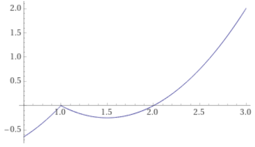
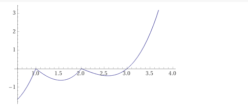
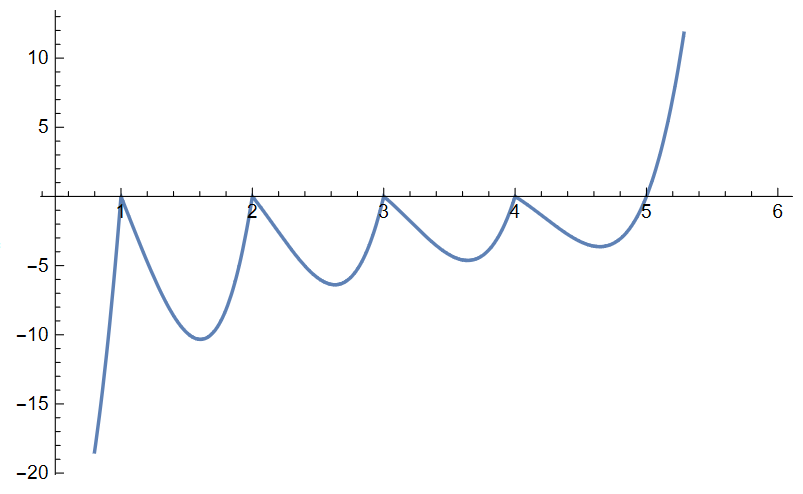
The sign of the eigenvalue (7) of the signature distribution is as follows:

(8)$$\!\!\!\!\!\!\!\!\!\!\!\!\!\!\!\!\!\!\!\!\!\!\!\!\!\!\!\! \!\!\!\!\!\!\!\!\!\!\!\!\!\!\!\!\!\!\!\!\!\!\!\!\!\!\!\! \!\!\!\!\!\!\!\!\!\!\!\!\!\!\!\!\!\!\!\!\!\!\!\!\!\!\!\! \!\!\!\!\!\!\!\!\!\!\!\!\!\!\!\!\!\!\!\!\!\!\!\!\!\!\!\! \!\!\!\!\!\!\!\!\!\!\!\!\!\!\!\!\!\!\!\!\!\!\!\!\!\!\!\! \!\!\!\!\!\!\!\!\!\!\!\!\!\!\!\!\!\!\!\!\!\!\!\!\!\!\!\! EV \big( (sgn(\sigma))_{\sigma \in Sym(n)} \big) \;is\; \left\{ \array{ \gt 0 & for & \mathrlap{ e^\beta \gt n-1 \;or\; e^{\beta} \in (n-2a-3, n-2a-2),\, a \in \mathbb{N} } \\ = 0 & for & \mathrlap{ e^\beta \in \{0,1,2, \cdots, n-1\} } \\ \lt 0 & for & \mathrlap{ e^{\beta} \in (n-2a-2, n-2a-1),\, a \in \mathbb{N} } } \right.$$

Proof

Since the prefactor $e^{- \beta \cdot n}$ in (7) is always positive, we need to equivalently discuss the sign of the polynomial

$$\underoverset {k = 0} {n - 1} {\prod}\big(e^{\beta} - k \big) \,.$$

Here the first two statements are immediate. For the last last statement, observe that all roots of the polynomial appear with unit multiplicity, so that the polynomial must change sign as $e^\beta$ crosses over any of its zeros. Therefore the value which is positive for $e^\beta \gt n-1$, by the first statement, must become negative as $e^\beta$ drops below $n=1$, then positive again as it drops below the next zero at $n - 2$, and negative once more as $e^\beta$ drops below $n - 3$, and so on.

General eigenvectors

The general eigenvectors and eigenvalues of the Cayley distance kernel are given as explicit expressions in the irreducible characters of the symmetric group, by the character formula of Cayley graph spectra:

To be able to apply this formula, one just has to observe that the exponentiated Cayley distance in a single variable

$$\array{ Sym(n) &\longrightarrow& \mathbb{R} \mathrlap{ \hookrightarrow \mathbb{C} } \\ \sigma &\mapsto& e^{- \beta \cdot d_C(\sigma,e)} }$$

is a class function for all $\beta$, which is immediate by Cayley’s observation that $d_c(\sigma,e) = n - \left\vert Cycles(\sigma)\right\vert$.

It thus follows from the general character formula and the representation theory of the symmetric group (here) that:

Proposition

(character formula for eigenvalues)
The eigenvalues of the Cayley distance kernel $e^{- \beta \cdot d_C}$ on $Sym(n)$ are:

1. labeled by partitions $\lambda$ of $n$:

   (9)$$\big( EigVals[e^{-\beta \cdot d_C}]_\lambda \big)_{\lambda \in Part(n)}$$

2. have multiplicity the square $\big(\chi^{(\lambda)}(e)\big)^2$ of the dimension of the $\lambda$th Specht module;

3. are given by

   (10)$$EigVals[e^{- \beta\cdot d_C}]_\lambda \;=\; \tfrac{1}{\chi^{(\lambda)}(e)} \underset{ \sigma \in Sym(n) }{\sum} e^{ \beta \cdot ( \left\vert Cycles(\sigma)\right\vert - n ) } \cdot \chi^{(\lambda)}(\sigma) \,,$$

   where $\chi^{(\lambda)}$ is the irreducible character corresponding to the $\lambda$th Specht module.

4. correspond to eigenvectors given by the complex conjugate of the $(i,j)$-components, for fixed $i,j \in \big\{1, \cdots, \chi^{(\lambda)}(e) \big\}$, of the $\lambda$th Specht module $S^{(\lambda)} \colon Sym(n) \to U\big(\chi^{(\lambda)}(e)\big)$ regarded for each permutation $\sigma$ as a unitary matrix $\big(S^{(\lambda)}(\sigma)_{i,j}\big)_{i,j}$:

   (11)$$\left\vert \lambda, (i,j) \right\rangle \;\coloneqq\; EigVects[e^{-\beta \cdot d_X}]_{\lambda, i, j} \;=\; \big( \bar S^{(\lambda)}(\sigma)_{i j} \big)_{\sigma \in Sym(n)} \;\; \in \; \mathbb{C}[Sym(n)] \,.$$

We further characterize these eigenvalues (Prop. below) at the special inverse temperatures of the form $\beta = ln(N)$. First we need some notation and a lemma:

Definition

(notation for sets of semistandard Young tableaux)
For $n, N \in \mathbb{N}$, write

$$ssYT_n(N) \;\in\; Set$$

for the set of semistandard Young tableau

• with $n$ boxes, and

• all labels $\leq N$.

Moreover for $\lambda \in Part(n)$ write

$$ssYT_{\lambda \vdash n}(N) \;\coloneqq\; \big\{ T \in ssYT_n(N) \;\vert\; \lambda = \left\vert T \right\vert \big\} \;\subset\; ssYT_{n}(N)$$

for the subset on those tableau $T$ whose underlying Young diagram $\left\vert T \right\vert$ corresponds to the partition $\lambda$.

Lemma

(character formula for integer exponential by cycle number)

For $N \in \mathbb{N}$ the exponential of $N$ to the number of cycles of a permutation is, as a class function, equal to the sum of irreducible characters weighted by the number of corresponding semistandard Young tableaux (Def. ):

$$N^{\left\vert Cycles(-) \right\vert} \;=\; \underset{ T \in ssYT_n(N) }{\sum} \chi^{ \left\vert T \right\vert }(-) \,.$$

This is the statement of Gnedin, Gorin & Kerov 11, Prop. 2.4 (with notation from Prop. 2.1).

Proposition

(Eigenvalues of Cayley distance kernel at $\beta = ln(N)$ count semistandard Young tableaux)

For $N \in \mathbb{N}$ and $\lambda \in Part(n)$, the $\lambda$th eigenvalue (9) of the Cayley distance kernel at $\beta = ln(N)$ on $Sym(n)$ is proportional to the number $\left\vert ssYT_{\lambda \vdash n}(N)\right\vert$ of semistandard Young tableaux (Def. )

(12)$$EigVals[e^{- ln(N) \cdot d_c}]_\lambda \;=\; \tfrac{n!}{N^n \cdot \chi^{(\lambda)}(e)} \left\vert ssYT_{\lambda}(N)\right\vert \,.$$

Proof

We compute as follows:

$$\begin{aligned} \mathrm{EigVals}[e^{-\mathrm{ln}(N) \cdot d_C}]_\lambda & \;=\; \frac{ e^{- \mathrm{ln}(N)\cdot n} }{ \chi^{(\lambda)}(e) } \underset{\sigma \in \mathrm{Sym}(n)}{\sum} \chi^{(\lambda)}(\sigma) \cdot N^{\# \mathrm{cycles}(\sigma)} \\ & \;=\; \frac{ e^{- \mathrm{ln}(N)\cdot n} }{ \chi^{(\lambda)}(e) } \underset{\sigma \in \mathrm{Sym}(n)}{\sum} \chi^{(\lambda)}(\sigma) \cdot \big( N \cdot 1^{\ell_1(\sigma)} \big) \big( N \cdot 1^{\ell_2(\sigma)} \big) \cdots \big( N \cdot 1^{\ell_{\#\mathrm{cycles}(\sigma)}(\sigma)} \big) \\ & \;=\; n! \frac{ e^{- \mathrm{ln}(N)\cdot n} }{ \chi^{(\lambda)}(e) } \cdot s_\lambda \big( x_1 \!=\! 1, \cdots, x_N \!=\! 1 \big) \\ & \;=\; n! \frac{ e^{- \mathrm{ln}(N)\cdot n} }{ \chi^{(\lambda)}(e) } \, \cdot \, \# \mathrm{ssYT}_\lambda\!(N) \,. \end{aligned}$$

Here

• the first line is the character formula for kernel spectra (10),

• the third step is the character formula for Schur polynomials,

• the last step is their counting property.

Alternatively, using Lemma we may compute as follows:

$$\begin{aligned} EigVals[e^{- ln(N) \cdot d_C}]_\lambda & \;=\; \tfrac{1}{\chi^{(\lambda)}(e)} \underset{\sigma \in Sym(n)}{\sum} e^{ ln(N) ( \left\vert Cycles(\sigma) \right\vert ) - n } \cdot \chi^{(\lambda)}(\sigma) \\ & \;=\; \tfrac{1}{\chi^{(\lambda)}(e)} \underset{\sigma \in Sym(n)}{\sum} e^{ ln(N) ( \left\vert Cycles(\sigma) \right\vert ) - n } \cdot \bar \chi^{(\lambda)}(\sigma) \\ & \;=\; \tfrac{1}{N^n \cdot \chi^{(\lambda)}(e)} \underset{\sigma \in Sym(n)}{\sum} N^{ \left\vert Cycles(\sigma) \right\vert } \cdot \bar \chi^{(\lambda)}(\sigma) \\ & \;=\; \tfrac{1}{N^n \cdot \chi^{(\lambda)}(e)} \underset{ T \in ssYT_n(N) }{\sum} \underset{\sigma \in Sym(n)}{\sum} \chi^{ \left\vert T \right\vert }(\sigma) \cdot \bar \chi^{(\lambda)}(\sigma) \\ & \;=\; \tfrac{n!}{N^n \cdot \chi^{(\lambda)}(e)} \underset{ T \in ssYT_n(N) }{\sum} \delta^{ \left\vert T\right\vert, \lambda } \end{aligned}$$

Here the first line is the character expression (10) of the eigenvalues from Prop. . The second line passes to the complex conjugation using that all eigenvalues are real (the Cayley distance kernel being a real symmetric matrix). The fourth step inserts the character formula from Lemma . The last step follows with Schur orthogonality (this equation).

As a corollary we obtain:

Proposition

(non-negativity of Cayley distance kernel at log-integer inverse temperature)

For the Cayley distance kernel at $\beta = ln(N)$ with $N \in \mathbb{N}$:

1. all eigenvalues (9) are non-negative

   $$\underset{\lambda \in Part(n)}{\forall} \, EigVals[e^{- ln(N) \cdot d_c}]_\lambda \;\geq\; 0 \,;$$

2. zero is an eigenvalue for $N \lt n$

   $$N \leq n - 1 \;\;\;\;\;\;\; \Rightarrow \;\;\;\;\;\;\; \underset{\lambda \in Part(n)}{\exists} \, EigVals[e^{- ln(N) \cdot d_c}]_\lambda \;=\; 0 \,;$$

3. all eigenvalues are positive if $N \geq n$:

   $$N \geq n \;\;\;\;\;\;\; \Rightarrow \;\;\;\;\;\;\; \underset{\lambda \in Part(n)}{\forall} \, EigVals[e^{- ln(N) \cdot d_c}]_\lambda \;\gt\; 0 \,.$$

Proof

By (12) in Prop. the eigenvalues at $\beta = ln(N)$ count possible numbers of colorings of Young diagrams to semistandard Young tableaux (ssYT). This gives the first statement.

Since in a ssYT the labels must strictly increase downwards, there is no possible ssYT-coloring if there are fewer labels than rows. This gives the second claim.

But conversely, since in an ssYT the labels may be constant horizontally, there is at least one coloring once there never are more rows than labels. This gives the last claim.

We give further combinatorial expressions of the eigenvalues of the Cayley distance kernel, using the hook length formula and the hook-content formula:

Proposition

(Eigenvalues of Cayley distance kernel via hook-content formula)

The eigenvalues (10) of the Cayley distance kernel for all $e^\beta \in \mathbb{R}_+$ may be expressed as:

$$EigVals[e^{- \beta \cdot d_C}]_\lambda \;=\; \frac {n!} {\chi^{(\lambda)}} e^{- \beta \cdot N} \underset { { 1 \leq i \leq rows(\lambda) } \atop { 1 \leq j \leq \lambda_i } } {\prod} \frac{ e^{\beta}+ j - i }{ \ell hook_\lambda(i,j) } \,.$$

The following proof was pointed out by Abdelmalek Abdesselam.

Proof

By Prop. the $\lambda$th eigenvalue at integer values

$$e^{\beta} = N \in \mathbb{N}_+$$

is a positive multiple of the number of semi-standard Young tableau, and hence is given by the hook-content formula, as follows:

$$\begin{aligned} \frac { \chi^{(\lambda)}(e) } { n! } N^n \cdot EigVals[e^{- ln(N)} \cdot d_C]_\lambda & \;=\; \left\vert ssYT_\lambda(N) \right\vert \\ & \;=\; \underset{(i,j)}{\prod} \frac { N + content(i,j) } { \ell hook_\lambda(i,j) } \end{aligned} \,, {\phantom{AAAA}} N \in \mathbb{N}_+ \,.$$

We may regard this set of equations as the specialization of the following more general equation

$$\frac { \chi^{(\lambda)}(e) } { n! } (e^\beta)^n \cdot EigVals[e^{- \beta} \cdot d_C]_\lambda \;=\; \underset{(i,j)}{\prod} \frac { e^\beta + content(i,j) } { \ell hook_\lambda(i,j) }$$

to all integer values of $e^\beta$. But since both sides of this equation are polynomials in $e^\beta$ – the right hand manifestly so, the left hand side by (10) – the fact that the equation holds at infinite many distinct points $e^\beta \in \mathbb{N}_+$ implies that in fact it holds for all $e^\beta \in \mathbb{R}_+$.

In fact:

Proposition

(Eigenvalues if Cayley distance kernel in terms of just box content)
The Eigenvalues (10) of the Cayley distance kernel for all $e^\beta \in \mathbb{R}_+$ may be expressed as:

$$EigVals[e^{- \beta \cdot d_C}]_\lambda \;=\; e^{- \beta \cdot N} \underset { { 1 \leq i \leq rows(\lambda) } \atop { 1 \leq j \leq \lambda_i } } {\prod} \big( e^{\beta}+ j - i \big) \,.$$

This is essentially, the result of Jucys 71, see at Jucys-Murphy element.

Proof

The point is that the hook length formula (see here) also gives the dimension of the irreps of the symmetric group:

(13)$$\chi^{(\lambda)}(e) \;=\; dim \big( S^{(\lambda)} \big) \;=\; \frac { n! } { \underset{(i,j)}{\prod} \ell hook_\lambda(i,j) } \,.$$

Using this, we compute as follows:

$$\begin{aligned} EigVals[e^{- \lambda \cdot d_C}]_\lambda & \;=\; \frac {n!} {\chi^{(\lambda)}} e^{- \beta \cdot N} \underset { { 1 \leq i \leq rows(\lambda) } \atop { 1 \leq j \leq \lambda_i } } {\prod} \frac{ e^{\beta}+ j - i }{ \ell hook_\lambda(i,j) } \\ & \;=\; e^{- \beta \cdot N} n! \frac { \underset{(i,j)}{\prod} \ell hook_\lambda(i,j) } {n!} \underset { (i,j) } {\prod} \frac{ e^{\beta}+ j - i }{ \ell hook_\lambda(i,j) } \\ & \;=\; e^{- \beta \cdot N} \underset { { 1 \leq i \leq rows(\lambda) } \atop { 1 \leq j \leq \lambda_i } } {\prod} \big( e^{\beta}+ j - i \big) \,. \end{aligned}$$

Here the first line is Prop. and the second step inserts (13).

Dual basis

We make explicit the inner product with respect to which the Cayley distance kernel is a hermitian matrix:

Definition

(Cartesian inner product)

Let

$$\array{ \mathbb{C}[Sym(n)] \times \mathbb{C}[Sym(n)] & \overset{ \;\;\;\;\;\; \langle -,-\rangle \;\;\;\;\;\; }{ \longrightarrow } & \mathbb{C} \\ \Big( \big( v_1(\sigma) \big)_{\sigma \in Sym(n)}, \; \big( v_2(\sigma') \big)_{\sigma' \in Sym(n)} \Big) & \mapsto & \underset{\sigma \in Sym(n)}{\sum} \bar v_1(\sigma) \cdot v_2(\sigma) }$$

denote the sesquilinear form induced by the canonical linear basis of the linear span $\mathbb{C}[Sym(n)]$.

Proposition

(dual eigenvector basis)

With respect to the Cartesian inner product from Def. , the eigenvectors (11) from Prop. have a dual basis given by

(14)$$\left\langle \lambda, (i, j) \right\vert \;\coloneqq\; \frac { \chi^{(\lambda)}(e) } { n! } EigVects[e^{- \beta \cdot d_C}]_\lambda \;=\; \frac { \chi^{(\lambda)}(e) } { n! } \big( \bar S^{(\lambda)}_{i j}(\sigma) \big)_{\sigma \in Sym(n)} \,.$$

Beware that the original eigenvector basis (11) already involves the complex conjugate $\bar S$ of component entries.

Proof

This is a restatement of the Schur orthogonality relation for irreps, here for the Specht modules $S^{(\lambda)}$:

We compute as follows:

$$\begin{aligned} \big\langle \lambda_1, (i_1, j_1) \big\vert \lambda_2, (i_2, j_2) \big\rangle & \;=\; \frac{ \chi^{(\lambda_1)}(e) }{ n! } \underset{\sigma \in Sym(n)}{\sum} S^{(\lambda_1)}(\sigma)_{j_1 i_1} \overline{ S^{(\lambda_2)}(\sigma)_{i_2 j_2} } \\ & \;=\; \delta^{\lambda_1 \lambda_2} \delta_{i_1 i_2} \delta_{j_1 j_2} \,. \end{aligned}$$

Here the first step unwinds the definitions (using (14) and (11) in Def. ), and the last step is the grand Schur orthogonality relation (?).

Positivity

We discuss at which values of the inverse temperature $\beta$, the Cayley distance kernel on $Sym(n)$ is, as a bilinear form, indefinite or positive (semi-)definite.

Indefiniteness for $e^{\beta} \in (0,1) \cup (1,2) \cup \cdots \cup (n-2,n-1)$

Proposition

For all $n \geq 3$ and all $0 \lt \beta \lt ln(2)$, the Cayley distance kernel $e^{- \beta \cdot d_C}$ fails to be positive semi-definite on $Sym(n)$.

Proof

By Example the statement holds for $n = 3$. But the kernel for this case is a principal submatrix of the kernels in all other cases (see this Prop.), and positivity fails as soon as it fails on any principal submatrix. (This is immediate from the definition, but also a direct consequence of Cauchy's interlace theorem.)

More generally:

Proposition

The Cayley distance kernel $e^{- \beta \cdot d_C}$ (Def. ) on $Sym(n)$ is indefinite for all

$$e^{\beta} \;\in\; (0,1) \cup (1,2) \cup \cdots \cup (n-2, n-1) \,,$$

or equivalently:

For $0 \lt e^\beta \lt n-1$ the Cayley distance kernel is indefinite except possibly at integer values.

Proof

With the third statement in Lemma the claim follows for every second open unit interval between 0 and $n-1$. But by the same argument the analogous statement is then true on every other of these unit intervals for the kernel on $Sym(n-1)$. Now since the kernel on $Sym(n-1)$ is a principal submatrix of that for $Sym(n)$ (see this Prop.), the Cauchy interlace theorem implies that the kernel on $Sym(n)$ must have a negative eigenvalue as soon as that on $Sym(n-1)$ does.

Semi-definiteness for $e^\beta \in \{1,2,\cdots, n-1\}$

Lemma

For $e^\beta = N \in \{1, 2, \cdots, n-1\}$ all the eigenvalues of the Cayley distance kernel $e^{- \beta \cdot d_C}$ on $Sym(n)$ are non-negative and for $e^\beta = n$ they are all positive.

Proof

We observe that the eigenvalues at these particular values of $\beta$ appear, up to a positive multiple, as coefficients of monomials in Schur polynomials, but all such coefficients are non-negative integers (this Prop.).

Concretely, for $\lambda$ any partition of $n$, with corresponding Schur polynomial $\s_\lambda$ and irreducible Specht character $\chi^{(\lambda)}$, consider the following computation:

(15)$$\begin{aligned} s_{\lambda} \big( \underset{ N \; args }{ \underbrace{ x, x, \cdots, x } } , \underset{ n - N \; args }{ \underbrace{ 0, 0, \cdots, 0 } } \big) & \;=\; \frac{1}{n!} \underset{ \sigma \in Sym(n) }{\sum} \chi^{(\lambda)}(\sigma) \cdot \big( N x^{l_1} \big) \big( N x^{l_2} \big) \cdots \big( N x^{l_{\left\vert Cycles(\sigma)\right\vert}} \big) \\ & \;=\; \left( \frac{1}{n!} \underset{ \sigma \in Sym(n) }{\sum} \chi^{(\lambda)}(\sigma) \cdot N^{ \left\vert Cycles(\sigma) \right\vert } \right) \cdot x^n \\ & \;=\;\; \underset{ \in \, \mathbb{N} }{ \underbrace{ \left( \tfrac {\chi^{(\lambda)}(1)} {n!} e^{ln(N) \cdot n} \cdot EV_\lambda (e^{- ln(N) \cdot d_C}) \right) } } \cdot x^n \end{aligned}$$

Here we used:

1. the Frobenius formula for Schur functions (this Prop.);

2. some evident re-arrangements;

3. the character formula for the eigenvalues (this Prop).

This shows the first part of the statement. Finally, that the eigenvalues for $e^\beta = N$ are in fact positive follows since in this case all the arguments $x_i$ on the top left of (15) are non-vanishing, so that none of the monomials contributing to $x^n$ vanishes.

Proposition

For $e^\beta = N \in \{1,2, \cdots, n-1\}$ the Cayley distance kernel $e^{- \beta \cdot d_C}$ is positive semi-definite.

For $e^{\beta} = n$ it is positive definite.

Proof

By Lemma the eigenvalues at all these values are non-negative and positive for the special case $e^{\beta} = n$, while by Lemma they do contain 0 away from this special case.

Alternatively, this follows from Prop. .

Definiteness for $e^\beta \in \{n, n+1 , n+2, \cdots \}$

Proposition

The Cayley distance kernel on $Sym(n)$ is positive definite for all $e^\beta \in \{n, n+1, n+2, \cdots\}$.

Proof

By Prop. the CD kernel on $Sym(n + k)$ is positive definite at $e^\beta = n + k$, which holds for all $k \in \mathbb{N}$. But the CD kernel in question is a principal submatrix of this positive one (see this Prop.), and hence cannot be less than positive itself, by the Cauchy interlace theorem.

Alternatively, this follows from the third clause of Prop.

Definiteness for $\e^\beta \gt n$

Proposition

The Cayley distance kernel $e^{- \beta \cdot d_C}$ on $Sym(n)$ is positive definite for $e^\beta \gt n - 1$.

Proof

With the $\lambda$th eigenvalue expressed either via Prop. or Prop. , it is manifest that a sufficient condition for their positivity is clearly that

$$e^\beta + content(i,j) \;\coloneqq\; e^{\beta} + j - i \;\gt\; 0$$

for all $(i,j)$ that appear in the product, hence that

$$e^{\beta} + 1 - i \;\gt\; 0$$

for all $i$ that appear. But the index $i$ labels the rows of Young diagrams of $n$ boxes, and hence the condition is that

$$e^{\beta} \;\gt\; \underset{ { \lambda \in Part(n) } \atop { 1 \leq i \leq rows(\lambda) } }{max} (i - 1) \;=\; n - 1 \,.$$

The following is an alternative proof of a much weaker lower bound, not relying on the hook-content formula from combinatorics, but on the Gershgorin circle theorem from analysis:

Proposition

A sufficient condition for the Cayley distance kernel (Def. ) on $Sym(n)$ to be positive definite is that its inverse temperature $\beta$ satisfies the following inequality:

(16)$$\underoverset {k = 0} {n - 1} {\prod} \big( e^{\beta} + k \big) \;\lt\; 2 e^{\beta \cdot n } \,.$$

Proof

By the Gershgorin circle theorem and using Prop. , all the eigenvalues of the kernel are within a distance $r(\beta)$ (6) from its diagonal values, which are all equal to $1 = e^{- \beta \cdot 0}$. Since, moreover, all eigenvalues are real, the condition

(17)$$\begin{aligned} r(\beta) \;=\; e^{- \beta \cdot n } \, \underoverset {k = 0} {n - 1} {\prod} \big( e^{\beta} + k \big) - 1 & \;\;\lt\;\; 1 \\ \Leftrightarrow \;\;\; e^{- \beta \cdot n } \, \underoverset {k = 0} {n - 1} {\prod} \big( e^{\beta} + k \big) & \;\;\lt\;\; 2 \end{aligned}$$

implies that all eigenvalues are contained in the interval $(0,2) \subset \mathbb{R}$ and hence in particular that they are positive.

Proposition

For inverse temperature being the natural logarithm of a natural number

(18)$$\beta \;=\; \ln(N) \,, \;\;\; N \,\in\, \mathbb{N}$$

a sufficient condition for the Cayley distance kernel (Def. ) to be positive semi-definite on $Sym(n)$ is that

$$N \;\gt\; \frac{ n-1 }{ q^{1/n} - 1 }$$

for $q = 3$.

Proof

First consider the case of $q =2$:

In the given case (18) the Gershgorin bound (16) for positive semi-definity of the Cayley distance kernel reads

$$\underset{ = (N + n - 1)! / (N - 1)! }{ \underbrace{ N (N + 1) (N + 2) \cdots (N + n - 1) } } \;\lt\; 2 N^n$$

and hence may equivalently be expressed as

(19)$$\array{ & \frac{ N (N + 1 ) \cdots (N + n -1) }{ N^n } & \;\lt\; 2 \\ \Leftrightarrow & \left( { N + n - 1 } \atop { N -1 } \right) \cdot \frac{ n ! }{ N^n } & \;\lt\; 2 } \;\;\;\;\;\; \Rightarrow \;\;\;\;\;\; e^{- ln(N) \cdot d_C} \, \text{is positive definite on} \, Sym(n) \,.$$

With the evident bound

$$\frac{ N (N + 1 ) \cdots (N + n -1) }{ N^n } \;\leq\; \left( \frac{ N + n - 1 }{ N } \right)^n \;=\; \left( 1 + \frac{ n - 1 }{ N } \right)^n \,,$$

the condition (19) is satisfied as soon as

$$\begin{aligned} & \left( 1 + \frac{ n - 1 }{ N } \right)^n \;\lt\; 2 \\ \Leftrightarrow \;\;\; & N \;\gt\; \frac{ n-1 }{ 2^{1/n} - 1 } \end{aligned}$$

Now to improve this to $q =3$: Since we may assume that at least $N \gt n-1$, we know that the eigenvalues of the homogeneous distribution (Example ) and of the signature distribution (Prop. ) are non-negative (by Lemma ). But by the character formula for Cayley graph spectra (this Prop) these are precisely the two eigenvalues with unit multiplicity. Therefore a strengthening of the Gershgorin circle theorem applies to all the remaining eigenvalues, saying (this Prop.) that these are in fact within half the Gershgorin radius (6). This allows us to put a factor of 1/2 on the left hand side of the first row of (17), which amounts to replacing the “2” by a “3” on the right of the second row.

Remark

Computer-experiment suggests (CSS21, Bar-Natan 21) that the above bounds (Prop. ) are rather loose: For the first few values of $N$, at least, the inverse temperature $\beta \geq ln(N-1)$ is already sufficient for positive semi-definiteness.

Cayley state on the group algebra

under construction

We observe that for $e^\beta \in \mathbb{R}_+$ integral or greater than $n-1$, the Cayley distance kernel $e^{- \beta \cdot d_C}$ defines a quantum state (in the sense of state on a star-algebra)

$$\big\langle - \big\rangle_\beta \;\colon\; \mathbb{C}[Sym(n)] \longrightarrow \mathbb{C}$$

on the group algebra canonically regarded as a star algebra. Then we exhibit it as a mixed state given by a probability distribution on pure states which are labeled by standard Young tableaux.

unpolished notes

The algebra

We regard the linear span $\mathbb{C}[Sym(n)]$ as equipped with the sesquilinear form given by

$$(a_1 \sigma_1, a_2 \sigma_2) \;\coloneqq\; \bar a_1 \, a_2 \, \delta_{\sigma_1, \sigma_2} \,, \;\;\;\;\; for \; a_1, a_2 \in \mathbb{C}, \; \sigma_1, \sigma_2 \in Sym(n) \,.$$

We regard any linear endomorphism $\phi$ on the linear span $\mathbb{C}[Sym(n)]$ as a matrix $[\phi]$ with respect to the canonical linear basis

$$[\phi]_{\sigma_1, \sigma_2} \;\coloneqq\; \big( \sigma_1, \phi(\sigma_2) \big) \,.$$

We denote matrix multiplication by “$\cdot$”, so that

$$[ \phi_2 \circ \phi_1 ] \;=\; [\phi_2] \cdot [\phi_1] \,.$$

Next, with $\mathbb{C}[Sym(n)]$ regarded as the group algebra, we will write the algebra product as $\bullet$.

This way, for $A_1, A_2 \in \mathbb{C}[Sym(n)]$ and with any element of the group algebra conflated with the endomorphism of left multiplication by this element, we have

$$[ A \bullet B] \;=\; [A] \cdot [B]$$

Notice that in this notation

$$A \;=\; A \bullet e \;=\; [A] \cdot e \,,$$

reflecting that $e \in \mathbb{C}[Sym(n)]$ is a cyclic vector.

Finally, we consider $\mathbb{C}[Sym(n)]$ as a complex star-algebra via

$$(a \, \sigma)^\ast \;=\; \bar a \, \sigma^{-1} \,.$$

Noticing

$$\big( [A^\ast] \cdot [\sigma_1] ,\, [\sigma_2] \big) \;=\; a_{ \sigma_1 \sigma_2^{-1} } \;=\; \big( [\sigma_1] ,\, [A]\cdot [\sigma_2] \big)$$

we see that

$$[A]^\dagger \;=\; \big[ A^\ast \big]$$

and so that

$$\mathbb{C}[Sym(n)] \overset{ [-] }{\longrightarrow} Mat(n! \times n!, \mathbb{C})$$

is a homomorphism of complex star-algebras.

The state

For

$$e^\beta \in \{1,2, \cdots, n-1\} \cup \mathbb{R}_{\gt n-1}$$

a state on this algebra is given by sending any

$$A \;=\; \underset{\sigma \in Sym(n)}{\sum} a_\sigma \sigma$$

to

$$\big\langle A \big\rangle_{\beta} \;\coloneqq\; \big( e, [e^{-\beta \cdot d_C}] \cdot A \big) \;\coloneqq\; \underset{ \sigma \in Sym(n) }{\sum} a_\sigma \cdot e^{ -\beta \cdot d_C(e, \sigma ) } \;=\; e^{- \beta \cdot n} \underset{ \sigma \in Sym(n) }{\sum} a_\sigma \cdot e^{ \beta \cdot \# cycles(\sigma) } \,.$$

This is indeed a state, because

$$\begin{aligned} \big\langle A^\ast \bullet A \big\rangle_{\beta} & \;\coloneqq\; \Big( e, \big[ e^{-\beta \cdot d_C} \big] \cdot (A^\ast \bullet A ) \Big) \\ & \;\coloneqq\; \underset{ \sigma_1, \sigma_2 \in Sym(n) }{\sum} \bar a _{\sigma_1} a_{\sigma_2} \cdot e^{ -\beta \cdot d_C(e, \sigma_1^{-1} \sigma_2 ) } \\ & \;=\; \underset{ \sigma_1, \sigma_2 \in Sym(n) }{\sum} \bar a _{\sigma_1} a_{\sigma_2} \cdot e^{ -\beta \cdot d_C(\sigma_1, \sigma_2 ) } \\ & \;=\; \Big( A, \, [e^{- \beta \cdot d_C}] \cdot A \Big) \\ & \;\geq \; 0 \end{aligned}$$

by left-invariance and by positive (semi-)definity of the Cayley distance kernel at the given $\beta$.

Idempotent decomposition

Regarding $\mathbb{C}[Sym(n)]$ as the regular representation of $Sym(n)$ it decomposes into irreps (Specht modules) $S^{(\lambda)}$ with multiplicity their dimension.

For $\lambda \in Part(n)$ and $1 \leq i \leq dim\big( S^{(\lambda)}\big)$ write

$$P^{(\lambda)}_i \;\colon\; \mathbb{C}[Sym(n)] \longrightarrow \mathbb{C}[Sym(n)]$$

for the linear projection onto the linear span of

$$\left\{ \underset{ \sigma \in Sym(n) }{\sum} \bar S^{(\lambda)}_{k i}(\sigma) \sigma \;\in\; \mathbb{C}[Sym(n)] \right\} _{ 1 \leq k \leq dim(S^{(\lambda)}) } \,.$$

Thus

$$\underset{ { \lambda \in Part(n) } \atop {1 \leq i_\lambda \leq dim(S^{(\lambda)})} }{ \sum } P^{(\lambda)}_{i_\lambda} \;=\; id \,.$$

Notice that each $P^{(\lambda)}_{j_\lambda}\big( \mathbb{C}[Sym(n)] \big)$ is a left ideal of the group algebra:

$$\begin{aligned} \sigma' \;\bullet\; \left( \underset{ \sigma \in Sym(n) }{\sum} \bar S^{(\lambda)}(\sigma)_{i j} \, \sigma \right) & \;=\; \underset{ \sigma \in Sym(n) }{\sum} \bar S^{(\lambda)}(\sigma)_{i j} \, \sigma' \bullet \sigma \\ & = \underset{ \sigma \in Sym(n) }{\sum} \bar S^{(\lambda)}( (\sigma')^{-1} \sigma)_{i j} \, \sigma \\ & \;=\; \underset{ \sigma \in Sym(n) }{\sum} \underset{ 1 \leq k \leq dim(S^{(\lambda)}) }{\sum} S^{(\lambda)}( \sigma' )_{i k} \bar S^{(\lambda)}( \sigma)_{k j} \, \sigma \\ & \;=\; \underset{ 1 \leq k \leq dim(S^{(\lambda)}) }{\sum} S^{(\lambda)}( \sigma' )_{i k} \left( \underset{ \sigma \in Sym(n) }{\sum} \bar S^{(\lambda)}( \sigma)_{k j} \, \sigma \right) \end{aligned}$$

Hence

$$\mathbb{C}[Sym(n)] \;\simeq\; \underset{ { \lambda \in Part(n) } \atop {1 \leq i_\lambda \leq dim(S^{(\lambda)})} }{\oplus} P^{(\lambda)}_i\big( \mathbb{C}[Sym(n)] \big)$$

is a decomposition into left ideals.

In fact, this is a decomposition into minimal ideals:

The minimal left ideals of any complex group algebra $\mathbb{C}[G]$ are labeled by pairs consisting of an irrep $V \in Rep(G)$ and a left ideal in the linear endomorphism algebra $End_{\mathbb{C}}(V)$ (by this Prop.). The latter is isomorphic to a matrix algebra and hence its left minimal ideals are the $dim(V)$-many single-column matrixes. Therefore minimal ideals in $\mathbb{C}[G]$ are labeled by pairs consisting of an irrep and a postitive natural number no larger than the dimension of the irrep. This is the same number/cardinality of ideals we found above, hence they must already be minimal.

(It’s also the same number of primitive idempotents as used in the discussion of Jucys-Murphy elements, see there.)

This decomposition of the group algebra into left ideals implies that for all $A \in \mathbb{C}[Sym(n)]$ we have

$$[P^{(\lambda)}_{i_\lambda}] \cdot [A] \;=\; [A] \cdot [P^{(\lambda)}_{i_\lambda}]$$

Moreover, we have

$$[e^{- \beta \cdot d_C}] \cdot [P^{(\lambda)}_{i_\lambda}] \;=\; [P^{(\lambda)}_{i_\lambda}] \cdot [e^{- \beta \cdot d_C}]$$

by the fact that the $\underset{ \sigma }{ \sum } \bar S^{(\lambda)}(\sigma) \, \sigma$ are eigenvectors of the Cayley distance kernel.

Finally, we have

$$\left( P^{(\lambda)}_{i_\lambda}( \bar S^{(\lambda_1)}_{i_1, j_1} ), \, \bar S^{(\lambda_2)}_{i_2, j_2} \right) \;=\; \left( \bar S^{(\lambda_1)}_{i_1, j_1}, \, P^{(\lambda)}_{i_\lambda} ( \bar S^{(\lambda_2)}_{i_2, j_2} ) \right)$$

hence

$$[P^{(\lambda)}_{i_\lambda}]^\dagger = [P^{(\lambda)}_{i_\lambda}]$$

(by grand Schur orthogonality, see this Prop.).

The mixture

Using the above properties of the projectors $[P^{(\lambda)}_{i_\lambda}]$, we observe that each

$$\big\langle - \big\rangle_{\beta, (\lambda, i_\lambda)} \;\coloneqq\; \frac{1}{ \big\langle P^{(\lambda)}_{i_\lambda}(e) \big\rangle_\beta } \, \big\langle P^{(\lambda)}_{i_\lambda}(-) \big\rangle_\beta$$

is still a state:

$$\begin{aligned} \big\langle P^{(\lambda)}_{i_\lambda}( A^\ast \bullet A) \big\rangle_\beta & \;=\; \big( e ,\, [e^{- \beta \cdot d_C}] \cdot [P^{(\lambda)}_{i_\lambda}] \cdot [A]^\dagger \cdot [A] \cdot e \big) \\ & \;=\; \big( e ,\, [e^{- \beta \cdot d_C}] \cdot [P^{(\lambda)}_{i_\lambda}] \cdot [P^{(\lambda)}_{i_\lambda}] \cdot [A]^\dagger \cdot [A] \cdot e \big) \\ & \;=\; \big( e ,\, [P^{(\lambda)}_{i_\lambda}] \cdot [e^{- \beta \cdot d_C}] \cdot [A]^\dagger \cdot [P^{(\lambda)}_{i_\lambda}] \cdot [A] \cdot e \big) \\ & \;=\; \big( P^{(\lambda)}(A) ,\, [e^{- \beta \cdot d_C}] \cdot P^{(\lambda)}_{i_\lambda}(A) \big) \\ & \;\geq\; 0 \end{aligned}$$

It follows that we have decomposed our state into a convex combination of other states as follows:

(20)$$\big\langle - \big\rangle_\beta \;=\; \underset{ { \lambda \in Part(n) } \atop {1 \leq i_\lambda \leq dim(S^{(\lambda)})} }{ \sum } p_{\lambda, i_\lambda} \cdot \big\langle - \big\rangle_{\beta, (\lambda, i_\lambda)} \,,$$

where

$$p_{\lambda, i_\lambda} \;\coloneqq\; \big\langle P^{(\lambda)}_{i_\lambda}(e) \big\rangle_\beta \,.$$

Claim. The $\langle - \rangle_{\beta, (\lambda, i_\lambda)}$ are pure states.

This must hold because the $P^{(\lambda)}_{i_\lambda}(\mathbb{C}[Sym(n)])$ are minimal ideals, by the discussion above, whence the projectors $P^{(\lambda)}_{i_\lambda}$ are given by left multiplication with primitive idempotents in the group algebra. Under the GNS construction, these correspond to projectors onto 1-dimensional subspaces, hence to pure states.

But this means that (20) exhibits our state as a mixture in which the $\lambda$th pure state appears with probability $p_{\lambda, i_\lambda}$.

The probability distribution

Now to express these probabilities more explicitly:

First observe the expansion of the neutral element in our eigenvector basis, evident from Schur orthogonality:

$$\begin{aligned} e & \;=\; \frac{1}{n!} \underset{\lambda, \sigma}{\sum} \chi^{(\lambda)}(e) \chi^{\lambda}(\sigma) \, \sigma \\ & \;=\; \frac{1}{n!} \underset{\lambda, \sigma, i}{\sum} \chi^{(\lambda)}(e) S^{\lambda}(\sigma)_{i i} \, \sigma \end{aligned} \,.$$

But this means that

$$\big( e, P^{(\lambda)}_i(e) \big) \;=\; \frac{1}{n!} \chi^{(\lambda)}(e) S^{(\lambda)}(e)_{i i} \;=\; \frac{\chi^{(\lambda)}(e)}{n!}$$

and so the probabilities are:

$$p_{\lambda, i} \;=\; \big( e, [e^{-\beta \cdot d_C}] \cdot P^{(\lambda)}_i(e) \big) \;=\; \frac{\chi^{(\lambda)}(e)}{n!} EigVals[e^{- \beta \cdot d_C}] \,.$$

As a sanity check, we have unit total probability:

$$\begin{aligned} \underset{\lambda, i}{\sum} p_{(\lambda,i)} & \;=\; \underset{\lambda}{\sum} \frac{\big(\chi^{(\lambda)}(e)\big)^2}{n!} EigVals[e^{- \beta \cdot d_C}] \\ & \;=\; \frac{1}{n!} \underset{ \lambda \in Part(n) }{\sum} \big( \chi^{(\lambda)}(e) \big)^2 \cdot \left( \frac{ 1 }{ \chi^{(\lambda)}(e) } \underset{\sigma \in Sym(n)}{\sum} e^{ \beta \cdot (\left\vert Cycles(\sigma) \right\vert - n ) } \cdot \chi^{(\lambda)}(\sigma) \right) \\ & \;=\; \frac{1}{n!} \underset{ \sigma \in Sym(n) }{\sum} e^{ \beta \cdot (\left\vert Cycles(\sigma) \right\vert - n ) } \underset{ = \delta_{e,\sigma} n! }{ \underbrace{ \underset{ \lambda \in Part(n) }{\sum} \chi^{(\lambda)}(e) \cdot \chi^{(\lambda)}(\sigma) } } \\ & \;=\; 1 \end{aligned}$$

In fact, by (12) in Prop. this is the probability distribution on Young diagrams with $n$ boxes proportionate to their number of semistandard Young tableaux with labels bounded by $N$:

(21)$$p^{Cay}_{\lambda, i} \;=\; \tfrac {\left\vert ssYT_{\lambda}(N)\right\vert} {N^n} \,.$$

If follows that the pushforward of this probality distribution along the forgetful function

(22)$$sYTableaux_n \overset{ q }{\longrightarrow} YDiagrams_n$$

is

$$q_\ast p \;:\; \lambda \;\mapsto\; \frac{ \left\vert sYTableaux_\lambda \right\vert \cdot \left\vert ssYTableaux_\lambda(N) \right\vert } {N^n} \;=\; \frac{ dim\big(S^{(\lambda)}\big) \cdot dim\big(V^{(\lambda)}\big) } {N^n} \,.$$

This is the Schur-Weyl measure.

Since the Cayley measure is constant on the fibers of $q$ (22) it is exactly that probability distribution on standard Yound tableaux which maximizes the entropy subject to the condition that the pushforward to Young diagrams is the Schur-Weyl measure.

Entropy of the Cayley state

Now to compute the von Neumann entropy of the Cayley state, hence the Shannon entropy of the above probability distribution:

$$S \;\coloneqq\; \underset{\lambda, i}{\sum} p^{Cay}_{\lambda, i} \ln \big( p^{Cay}_{\lambda, i} \big)$$

as a function of $n$.

Recall the bounds

Hartley entropy$\geq$ Shannon entropy $\geq$ min-entropy.

$$S_0 \;\geq\; S_1 \;geq\; S_\infty \,.$$

Hartley entropy

Observe that a Young diagram (partition) $\lambda$ admits a decoration to at least one semi-standard Young tableau with labels bounded by $N$ if and only if it has at most $N$ rows.

Therefore the Hartley entropy of the probability distribution (21) is the logarithm of the number of standard Young tableaux with $N$ boxes and at most $N$ rows:

$$S_0 \big( p^{Cay} \big) \;\; = \;\; sYT_n(N) \;\; \coloneqq \;\; ln \left( \underset { { \lambda \in Part(n) } \atop { rows(\lambda) \leq N } }{\sum} \underset{ \chi^{(\lambda)}(e) }{ \underbrace{ \left\vert sYT_\lambda \right\vert } } \right) \,.$$

For discussion of these numbers $\left\vert sYT_n(N) \right\vert$ see there.

(…)

Related concepts

• Mallows kernel, Kendall kernel, Markov kernel

• kernel method

References

Mentioning of the Cayley distance kernel:

• Michael A. Fligner, Joseph S. Verducci, Section 4 of: Distance Based Ranking Models, Journal of the Royal Statistical Society. Series B (Methodological) Vol. 48, No. 3 (1986), pp. 359-369 (jstor:2345433)

• Persi Diaconis, Phil Hanlon, Section 4 of: Eigen Analysis for Some Examples of the Metropolis Algorithm, in Donald Richards (ed.) Hypergeometric Functions on Domains of Positivity, Jack Polynomials, and Applications, Contemporary Mathematics Vol. 138, AMS 1992 (doi:10.1090/conm/138, EFS NSF 392, pdf)

• Michael A. Fligner, Joseph S. Verducci (eds.), p. xx of: Probability Models and Statistical Analyses for Ranking Data, Lecture Notes in Statistics 80, Springer 1993 (doi:10.1007/978-1-4612-2738-0)

The above discussion of the positivity of the Cayley distance kernel in dependence of the inverse temperature follows:

• David Corfield, Hisham Sati, Urs Schreiber: Fundamental weight systems are quantum states (arXiv:2105.02871)

Further computations in:

• Dror Bar-Natan, AcademicPensieve 2021-05, The Cayley distance kernel following arXiv://2105.0287 by Corfield, Sati, and Schreiber (nb, pdf, pdf)

Related discussion in:

• Iskander Azangulov, Viacheslav Borovitskiy, Andrei Smolensky On power sum kernels on symmetric groups [arXiv:2211.05650]

Supplementary references:

• Petteri Kaski, Eigenvectors and spectra of Cayley graphs, 2002 (pdf, pdf)

• Richard Stanley, Enumerative combinatorics – Volume 1, Wadsworth & Brooks/Cole Mathematics Series book series 1986, 1997 (doi:10.1007/978-1-4615-9763-6) reprinted in: Cambridge Studies in Advanced Mathematics, Cambridge University Press 2011 (ISBN:9781107602625, pdf)

• Alexander Gnedin, Vadim Gorin, Sergei Kerov, Block characters of the symmetric groups, Journal of Algebraic Combinatorics, 38, no. 1 (2013), 79-101 (arXiv:1108.5044, doi:10.1007/s10801-012-0394-9)