nLab Introduction to Topology -- 1

---

This page contains a detailed introduction to basic topology. Starting from scratch (required background is just a basic concept of sets), and amplifying motivation from analysis, it first develops standard point-set topology (topological spaces). In passing, some basics of category theory make an informal appearance, used to transparently summarize some conceptually important aspects of the theory, such as initial and final topologies and the reflection into Hausdorff and sober topological spaces. We close with discussion of the basics of topological manifolds and differentiable manifolds, hence of differential topology, laying the foundations for differential geometry.

$\,$

main page: Introduction to Topology

this chapter: Introduction to Topology 1 – Point-set topology

next chapter: Introduction to Topology 2 – Basic Homotopy Theory

$\,$

For introduction to more general and abstract homotopy theory see instead at Introduction to Homotopy Theory.

---

$\,$

$\,$

The idea of topology is to study “spaces” with “continuous functions” between them. Specifically one considers functions between sets (whence “point-set topology”, see below) such that there is a concept for what it means that these functions depend continuously on their arguments, in that their values do not “jump”. Such a concept of continuity is familiar from analysis on metric spaces, (recalled below) but the definition in topology generalizes this analytic concept and renders it more foundational, generalizing the concept of metric spaces to that of topological spaces. (def. below).

Hence, topology is the study of the category whose objects are topological spaces, and whose morphisms are continuous functions (see also remark below). This category is much more flexible than that of metric spaces, for example it admits the construction of arbitrary quotients and intersections of spaces. Accordingly, topology underlies or informs many and diverse areas of mathematics, such as functional analysis, operator algebra, manifold/scheme theory, hence algebraic geometry and differential geometry, and the study of topological groups, topological vector spaces, local rings, etc. Not the least, it gives rise to the field of homotopy theory, where one considers also continuous deformations of continuous functions themselves (“homotopies”). Topology itself has many branches, such as low-dimensional topology or topological domain theory.

A popular imagery for the concept of a continuous function is provided by deformations of elastic physical bodies, which may be deformed by stretching them without tearing. The canonical illustration is a continuous bijective function from the torus to the surface of a coffee mug, which maps half of the torus to the handle of the coffee mug, and continuously deforms parts of the other half in order to form the actual cup. Since the inverse function to this function is itself continuous, the torus and the coffee mug, both regarded as topological spaces, are “the same” for the purposes of topology; one says they are homeomorphic.

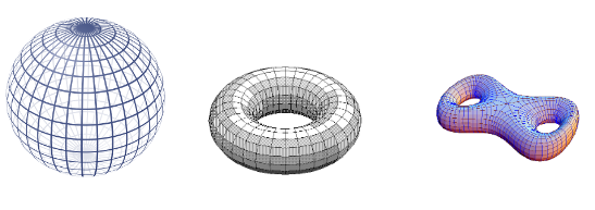
On the other hand, there is no homeomorphism from the torus to, for instance, the sphere, signifying that these represent two topologically distinct spaces. Part of topology is concerned with studying homeomorphism-invariants of topological spaces (“topological properties”) which allow to detect by means of algebraic manipulations whether two topological spaces are homeomorphic (or more generally homotopy equivalent) or not. This is called algebraic topology. A basic algebraic invariant is the fundamental group of a topological space (discussed below), which measures how many ways there are to wind loops inside a topological space.

Beware the popular imagery of “rubber-sheet geometry”, which only captures part of the full scope of topology, in that it invokes spaces that locally still look like metric spaces (called topological manifolds, see below). But the concept of topological spaces is a good bit more general. Notably, finite topological spaces are either discrete or very much unlike metric spaces (example below); the former play a role in categorical logic. Also, in geometry, exotic topological spaces frequently arise when forming non-free quotients. In order to gauge just how many of such “exotic” examples of topological spaces beyond locally metric spaces one wishes to admit in the theory, extra “separation axioms” are imposed on topological spaces (see below), and the flavour of topology as a field depends on this choice.

Among the separation axioms, the Hausdorff space axiom is the most popular (see below). But the weaker axiom of sobriety (see below) stands out, because on the one hand it is the weakest axiom that is still naturally satisfied in applications to algebraic geometry (schemes are sober) and computer science (Vickers 89), and on the other, it fully realizes the strong roots that topology has in formal logic: sober topological spaces are entirely characterized by the union-, intersection- and inclusion-relations (logical conjunction, disjunction and implication) among their open subsets (propositions). This leads to a natural and fruitful generalization of topology to more general “purely logic-determined spaces”, called locales, and in yet more generality, toposes and higher toposes. While the latter are beyond the scope of this introduction, their rich theory and relation to the foundations of mathematics and geometry provide an outlook on the relevance of the basic ideas of topology.

$\,$

In this first part we discuss the foundations of the concept of “sets equipped with topology” (topological spaces) and of continuous functions between them.

$\,$

(classical logic)

The proofs in the following freely use the principle of excluded middle, hence proof by contradiction, and in a few places they also use the axiom of choice/Zorn's lemma.

Hence we discuss topology in its traditional form with classical logic.

We do however highlight the role of frame homomorphisms (def. below) and that of sober topological spaces (def. below). These concepts pave the way to a constructive formulation of topology in terms not of topological spaces but in terms of locales (remark below). For further reading along these lines see Johnstone 83.

$\,$

(set theory)

Apart from classical logic, we assume the usual informal concept of sets. The reader (only) needs to know the concepts of

1. subsets$S \subset X$;

2. complements$X \setminus S$ of subsets;

3. image sets $f(X)$ and pre-image sets $f^{-1}(Y)$ under a function

   $f \colon X \to Y$;

4. unions$\underset{i \in I}{\cup} S_i$ and intersections $\underset{i \in I}{\cap} S_i$ of indexed sets of subsets $\{S_i \subset X\}_{i \in I}$.

The only rules of set theory that we use are the

1. interactions of images and pre-images with unions and intersections

2. de Morgan duality.

For reference, we recall these:

Proposition

(images preserve unions but not in general intersections)

Let $f \colon X \longrightarrow Y$ be a function between sets. Let $\{S_i \subset X\}_{i \in I}$ be a set of subsets of $X$. Then

1. $f\left( \underset{i \in I}{\cup} S_i\right) = \left(\underset{i \in I}{\cup} f(S_i)\right)$ (the image under $f$ of a union of subsets is the union of the images)

2. $f\left( \underset{i \in I}{\cap} S_i\right) \subset \left(\underset{i \in I}{\cap} f(S_i)\right)$ (the image under $f$ of the intersection of the subsets is contained in the intersection of the images).

The injection in the second item is in general proper. If $f$ is an injective function and if $I$ is non-empty, then this is a bijection:

• $(f\,\text{injective}) \Rightarrow \left(f\left( \underset{i \in I}{\cap} S_i\right) = \left(\underset{i \in I}{\cap} f(S_i)\right)\right)$

Proposition

(pre-images preserve unions and intersections)

Let $f \colon X \longrightarrow Y$ be a function between sets. Let $\{T_i \subset Y\}_{i \in I}$ be a set of subsets of $Y$. Then

1. $f^{-1}\left( \underset{i \in I}{\cup} T_i\right) = \left(\underset{i \in I}{\cup} f^{-1}(T_i)\right)$ (the pre-image under $f$ of a union of subsets is the union of the pre-images),

2. $f^{-1}\left( \underset{i \in I}{\cap} T_i\right) = \left(\underset{i \in I}{\cap} f^{-1}(T_i)\right)$ (the pre-image under $f$ of the intersection of the subsets is the intersection of the pre-images).

Proposition

(de Morgan's law)

Given a set $X$ and a set of subsets

$$\{S_i \subset X\}_{i \in I}$$

then the complement of their union is the intersection of their complements

$$X \setminus \left( \underset{i \in I}{\cup} S_i \right) \;\;=\;\; \underset{i \in I}{\cap} \left( X \setminus S_i \right)$$

and the complement of their intersection is the union of their complements

$$X \setminus \left( \underset{i \in I}{\cap} S_i \right) \;\;=\;\; \underset{i \in I}{\cup} \left( X \setminus S_i \right) \,.$$

Moreover, taking complements reverses inclusion relations:

$$\left( S_1 \subset S_2 \right) \;\;\Leftrightarrow\;\, \left( X\setminus S_2 \subset X \setminus S_1 \right) \,.$$

$\,$

Metric spaces

The concept of continuity was first made precise in analysis, in terms of epsilontic analysis on metric spaces, recalled as def. below. Then it was realized that this has a more elegant formulation in terms of the more general concept of open sets, this is prop. below. Adopting the latter as the definition leads to a more abstract concept of “continuous space”, this is the concept of topological spaces, def. below.

Here we briefly recall the relevant basic concepts from analysis, as a motivation for various definitions in topology. The reader who either already recalls these concepts in analysis or is content with ignoring the motivation coming from analysis should skip right away to the section Topological spaces.

Definition

(metric space)

A metric space is

1. a set $X$ (the “underlying set”);

2. a function $d \;\colon\; X \times X \to [0,\infty)$ (the “distance function”) from the Cartesian product of the set with itself to the non-negative real numbers

such that for all $x,y,z \in X$:

1. (symmetry) $d(x,y) = d(y,x)$

2. (triangle inequality) $d(x,z) \leq d(x,y)+ d(y,z)$.

3. (non-degeneracy) $d(x,y) = 0 \;\;\Leftrightarrow\;\; x = y$

Definition

(open balls)

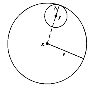
Let $(X,d)$, be a metric space. Then for every element $x \in X$ and every $\epsilon \in \mathbb{R}_+$ a positive real number, we write

$$B^\circ_x(\epsilon) \;\coloneqq\; \left\{ y \in X \;\vert\; d(x,y) \lt \epsilon \right\}$$

for the open ball of radius $\epsilon$ around $x$. Similarly we write

$$B_x(\epsilon) \;\coloneqq\; \left\{ y \in X \;\vert\; d(x,y) \leq \epsilon \right\}$$

for the closed ball of radius $\epsilon$ around $x$. Finally we write

$$S_x(\epsilon) \;\coloneqq\; \left\{ y \in X \;\vert\; d(x,y) = \epsilon \right\}$$

for the sphere of radius $\epsilon$ around $x$.

For $\epsilon = 1$ we also speak of the unit open/closed ball and the unit sphere.

Definition

For $(X,d)$ a metric space (def. ) then a subset $S \subset X$ is called a bounded subset if $S$ is contained in some open ball (def. )

$$S \subset B^\circ_x(r)$$

around some $x \in X$ of some radius $r \in \mathbb{R}$.

A key source of metric spaces are normed vector spaces:

Definition

(normed vector space)

A normed vector space is

1. a real vector space $V$;

2. a function (the norm)

   $${\Vert {-} \Vert} \;\colon\; V \longrightarrow \mathbb{R}_{\geq 0}$$

   from the underlying set of $V$ to the non-negative real numbers,

such that for all $c \in \mathbb{R}$ with absolute value ${\vert c \vert}$ and all $v , w \in V$ it holds true that

1. (linearity) ${\Vert c v \Vert} = {\vert c \vert} {\Vert v \Vert }$;

2. (triangle inequality) ${\Vert v+w \Vert} \leq {\Vert v \Vert } + {\Vert w \Vert}$;

3. (non-degeneracy) if ${\Vert v \Vert} = 0$ then $v = 0$.

Proposition

Every normed vector space $(V, {\Vert {-} \Vert})$ becomes a metric space according to def. by setting

$$d(x,y) \coloneqq {\Vert x-y \Vert} \,.$$

Examples of normed vector spaces (def. ) and hence, via prop. , of metric spaces include the following:

Example

(Euclidean space)

For $n \in \mathbb{N}$, the Cartesian space

$$\mathbb{R}^n = \left\{ \vec x = (x_i)_{i = 1}^n \vert x_i \in \mathbb{R} \right\}$$

carries a norm (the Euclidean norm ) given by the square root of the sum of the squares of the components:

$${\Vert \vec x \Vert} \;\coloneqq\; \sqrt{ \underoverset{i = 1}{n}{\sum} (x_i)^2 } \,.$$

Via prop. this gives $\mathbb{R}^n$ the structure of a metric space, and as such it is called the Euclidean space of dimension $n$.

Example

More generally, for $n \in \mathbb{N}$, and $p \in \mathbb{R}$, $p \geq 1$, then the Cartesian space $\mathbb{R}^n$ carries the p-norm

$${\Vert \vec x \Vert}_p \coloneqq \root p {\sum_i {|x_i|^p}}$$

One also sets

$${\Vert \vec x \Vert}_\infty \coloneqq \underset{i \in I}{max} \, {\vert x_i \vert}$$

and calls this the supremum norm.

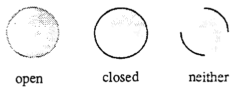
The graphics on the right (grabbed from Wikipedia) shows unit circles (def. ) in $\mathbb{R}^2$ with respect to various p-norms.

By the Minkowski inequality, the p-norm generalizes to non-finite dimensional vector spaces such as sequence spaces and Lebesgue spaces.

$\,$

Continuity

The following is now the fairly obvious definition of continuity for functions between metric spaces.

Definition

(epsilontic definition of continuity)

For $(X,d_X)$ and $(Y,d_Y)$ two metric spaces (def. ), then a function

$$f \;\colon\; X \longrightarrow Y$$

is said to be continuous at a point $x \in X$ if for every positive real number $\epsilon$ there exists a positive real number $\delta$ such that for all $x' \in X$ that are a distance smaller than $\delta$ from $x$ then their image $f(x')$ is a distance smaller than $\epsilon$ from $f(x)$:

$$\left( f\,\, \text{continuous at}\, x \right) \;\coloneqq\; \underset{{\epsilon \in \mathbb{R}} \atop {\epsilon \gt 0}}{\forall} \left( \underset{{\delta \in \mathbb{R}} \atop {\delta \gt 0}}{\exists} \left( \left( d_X(x,x') \lt \delta \right) \;\;\Rightarrow\;\; \left( d_Y(\,f(x), f(x')\,) \lt \epsilon \right) \right) \right) \,.$$

The function $f$ is said to be continuous if it is continuous at every point $x \in X$.

Example

(distance function from a subset is continuous)

Let $(X,d)$ be a metric space (def. ) and let $S \subset X$ be a subset of the underlying set. Define then the function

$$d(S,-) \;\colon\; X \to \mathbb{R}$$

from the underlying set $X$ to the real numbers by assigning to a point $x \in X$ the infimum of the distances from $x$ to $s$, as $s$ ranges over the elements of $S$:

$$d(S,x) \coloneqq inf \left\{ d(s,x) \,\vert\, s\in S \right\} \,.$$

This is a continuous function, with $\mathbb{R}$ regarded as a metric space via its Euclidean norm (example ).

In particular the original distance function $d(x,-) = d(\{x\},-)$ is continuous in both its arguments.

Proof

Let $x \in X$ and let $\epsilon$ be a positive real number. We need to find a positive real number $\delta$ such that for $y \in X$ with $d(x,y) \lt \delta$ then ${\vert d(S,x) - d(S,y) \vert} \lt \epsilon$.

For $s \in S$ and $y \in X$, consider the triangle inequalities

$$\begin{aligned} d(s,x) & \leq d(s,y) + d(y,x) \\ d(s,y) & \leq d(s,x) + d(x,y) \end{aligned} \,.$$

Forming the infimum over $s \in S$ of all terms appearing here yields

$$\begin{aligned} d(S,x) & \leq d(S,y) + d(y,x) \\ d(S,y) & \leq d(S,x) + d(x,y) \end{aligned}$$

which implies

$${\vert d(S,x) - d(S,y) \vert} \leq d(x,y) \,.$$

This means that we may take for instance $\delta \coloneqq \epsilon$.

Example

(rational functions are continuous)

Consider the real line $\mathbb{R}$ regarded as the 1-dimensional Euclidean space $\mathbb{R}$ from example .

For $P \in \mathbb{R}[X]$ a polynomial, then the function

$$\array{ f_P &\colon& \mathbb{R} &\longrightarrow& \mathbb{R} \\ && x &\mapsto& P(x) }$$

is a continuous function in the sense of def. . Hence polynomials are continuous functions.

Similarly rational functions are continuous on their domain of definition: for $P,Q \in \mathbb{R}[X]$ two polynomials, then $\frac{f_P}{f_Q} \colon \mathbb{R} \setminus \{x | f_Q(x) = 0\} \to \mathbb{R}$ is a continuous function.

Also for instance forming the square root is a continuous function $\sqrt(-) \colon \mathbb{R}_{\geq 0} \to \mathbb{R}_{\geq 0}$.

On the other hand, a step function is continuous everywhere except at the finite number of points at which it changes its value, see example below.

We now reformulate the analytic concept of continuity from def. in terms of the simple but important concept of open sets:

Definition

(neighbourhood and open set)

Let $(X,d)$ be a metric space (def. ). Say that:

1. A neighbourhood of a point $x \in X$ is a subset $U_x \subset X$ which contains some open ball $B_x^\circ(\epsilon) \subset U_x$ around $x$ (def. ).

2. An open subset of $X$ is a subset $U \subset X$ such that for every $x \in U$ it also contains an open ball $B^\circ_x(\epsilon)$ around $x$ (def. ).

3. An open neighbourhood of a point $x \in X$ is a neighbourhood $U_x$ of $x$ which is also an open subset, hence equivalently this is any open subset of $X$ that contains $x$.

The following picture shows a point $x$, some open balls $B_i$ containing it, and two of its neighbourhoods $U_i$:

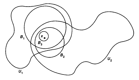
graphics grabbed from Munkres 75

Example

(the empty subset is open)

Notice that for $(X,d)$ a metric space, then the empty subset $\emptyset \subset X$ is always an open subset of $(X,d)$ according to def. . This is because the clause for open subsets $U \subset X$ says that “for every point $x \in U$ there exists…”, but since there is no $x$ in $U = \emptyset$, this clause is always satisfied in this case.

Conversely, the entire set $X$ is always an open subset of $(X,d)$.

Example

(open/closed intervals)

Regard the real numbers $\mathbb{R}$ as the 1-dimensional Euclidean space (example ).

For $a \lt b \in \mathbb{R}$ consider the following subsets:

1. $(a,b) \coloneqq \left\{ x \in \mathbb{R} \vert a \lt x \lt b \right\}$ $\phantom{AA}$ (open interval)

2. $(a,b] \coloneqq \left\{ x \in \mathbb{R} \vert a \lt x \leq b \right\}$ $\phantom{AA}$ (half-open interval)

3. $[a,b) \coloneqq \left\{ x \in \mathbb{R} \vert a \leq x \lt b \right\}$ $\phantom{AA}$ (half-open interval)

4. $[a,b] \coloneqq \left\{ x \in \mathbb{R} \vert a \leq x \leq b \right\}$ $\phantom{AA}$ (closed interval)

The first of these is an open subset according to def. , the other three are not. The first one is called an open interval, the last one a closed interval and the middle two are called half-open intervals.

Similarly for $a,b \in \mathbb{R}$ one considers

1. $(-\infty,b) \coloneqq \left\{ x \in \mathbb{R} \vert x \lt b \right\}$ $\phantom{AA}$ (unbounded open interval)

2. $(a,\infty) \coloneqq \left\{ x \in \mathbb{R} \vert a \lt x \right\}$ $\phantom{AA}$ $\,\,$ (unbounded open interval)

3. $(-\infty,b] \coloneqq \left\{ x \in \mathbb{R} \vert x \leq b \right\}$ $\phantom{AA}$ (unbounded half-open interval)

4. $[a,\infty) \coloneqq \left\{ x \in \mathbb{R} \vert a \leq x \right\}$ $\phantom{AA}$ $\,\,$ (unbounded half-open interval)

The first two of these are open subsets, the last two are not.

For completeness we may also consider

• $(-\infty , \infty) = \mathbb{R}$

• $(a,a) = \emptyset$

which are both open, according to def. .

We may now rephrase the analytic definition of continuity entirely in terms of open subsets (def. ):

Proposition

(rephrasing continuity in terms of open sets)

Let $(X,d_X)$ and $(Y,d_Y)$ be two metric spaces (def. ). Then a function $f \colon X \to Y$ is continuous in the epsilontic sense of def. precisely if it has the property that its pre-images of open subsets of $Y$ (in the sense of def. ) are open subsets of $X$:

$$\left( f \,\, \text{continuous} \right) \;\;\Leftrightarrow\;\; \left( \left( O_Y \subset Y \,\, \text{open} \right) \,\Rightarrow\, \left( f^{-1}(O_Y) \subset X \,\, \text{open} \right) \right) \,.$$

$\,$

principle of continuity

$\,$ $\,$ Continuous pre-Images of open subsets are open.

Proof

Observe, by direct unwinding the definitions, that the epsilontic definition of continuity (def. ) says equivalently in terms of open balls (def. ) that $f$ is continuous at $x$ precisely if for every open ball $B^\circ_{f(x)}(\epsilon)$ around an image point, there exists an open ball $B^\circ_x(\delta)$ around the corresponding pre-image point which maps into it:

$$\array{ \left( f \,\,\text{continuous at}\,\, x \right) & \Leftrightarrow \; \underset{\epsilon \gt 0}{\forall} \left( \underset{\delta \gt 0}{\exists} \left( f(\;B_x^\circ(\delta)\;) \;\subset\; B^\circ_{f(x)}(\epsilon) \right) \right) \\ & \Leftrightarrow \; \underset{\epsilon \gt 0}{\forall} \left( \underset{\delta \gt 0}{\exists} \left( B^\circ_x(\delta) \subset f^{-1}\left( B^\circ_{f(x)}(\epsilon) \right) \right) \right) } \,.$$

With this observation the proof immediate. For the record, we spell it out:

First assume that $f$ is continuous in the epsilontic sense. Then for $O_Y \subset Y$ any open subset and $x \in f^{-1}(O_Y)$ any point in the pre-image, we need to show that there exists an open neighbourhood of $x$ in $f^{-1}(O_Y)$.

That $O_Y$ is open in $Y$ means by definition that there exists an open ball $B^\circ_{f(x)}(\epsilon)$ in $O_Y$ around $f(x)$ for some radius $\epsilon$. By the assumption that $f$ is continuous and using the above observation, this implies that there exists an open ball $B^\circ_x(\delta)$ in $X$ such that $f(B^\circ_x(\delta)) \subset B^\circ_{f(x)}(\epsilon) \subset Y$, hence such that $B^\circ_x(\delta) \subset f^{-1}\left(B^{\circ}_{f(x)}(\epsilon)\right) \subset f^{-1}(O_Y)$. Hence this is an open ball of the required kind.

Conversely, assume that the pre-image function $f^{-1}$ takes open subsets to open subsets. Then for every $x \in X$ and $B_{f(x)}^\circ(\epsilon) \subset Y$ an open ball around its image, we need to produce an open ball $B_x^\circ(\delta) \subset X$ around $x$ such that $f(B_x^\circ(\delta)) \subset B^\circ_{f(x)}(\epsilon)$.

But by definition of open subsets, $B^\circ_{f(x)}(\epsilon) \subset Y$ is open, and therefore by assumption on $f$ its pre-image $f^{-1}(B^\circ_{f(x)}(\epsilon)) \subset X$ is also an open subset of $X$. Again by definition of open subsets, this implies that it contains an open ball as required.

Example

(step function)

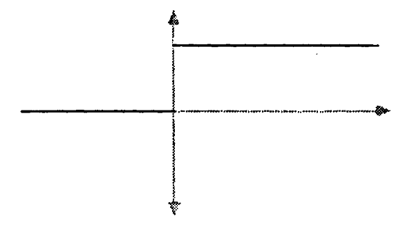
Consider $\mathbb{R}$ as the 1-dimensional Euclidean space (example ) and consider the step function

$$\array{ \mathbb{R} &\overset{H}{\longrightarrow}& \mathbb{R} \\ x &\mapsto& \left\{ \array{ 0 & \vert \, x \leq 0 \\ 1 & \vert \, x \gt 0 } \right. } \,.$$

graphics grabbed from Vickers 89

Consider then for $a \lt b \in \mathbb{R}$ the open interval $(a,b) \subset \mathbb{R}$, an open subset according to example . The preimage $H^{-1}(a,b)$ of this open subset is

$$H^{-1} \;\colon\; (a,b) \mapsto \left\{ \array{ \emptyset & \vert \, a \geq 1 \;\;\text{or} \;\; b \leq 0 \\ \mathbb{R} & \vert \, a \lt 0 \;\;\text{and}\;\; b \gt 1 \\ \emptyset & \vert \, a \geq 0 \;\;\text{and}\;\; b \leq 1 \\ (0,\infty) & \vert \, 0 \leq a \lt 1 \;\;\text{and}\;\; b \gt 1 \\ (-\infty, 0] & \vert \, a \lt 0 \;\;\text{and}\;\; b \leq 1 } \right. \,.$$

By example , all except the last of these pre-images listed are open subsets.

The failure of the last of the pre-images to be open witnesses that the step function is not continuous at $x = 0$.

$\,$

Compactness

A key application of metric spaces in analysis is that they allow a formalization of what it means for an infinite sequence of elements in the metric space (def. below) to converge to a limit of a sequence (def. below). Of particular interest are therefore those metric spaces for which each sequence has a converging subsequence: the sequentially compact metric spaces (def. ).

We now briefly recall these concepts from analysis. Then, in the above spirit, we reformulate their epsilontic definition in terms of open subsets. This gives a useful definition that generalizes to topological spaces, the compact topological spaces discussed further below.

Definition

(sequence)

Given a set $X$, then a sequence of elements in $X$ is a function

$$x_{(-)} \;\colon\; \mathbb{N} \longrightarrow X$$

from the natural numbers to $X$.

A sub-sequence of such a sequence is a sequence of the form

$$x_{\iota(-)} \;\colon\; \mathbb{N} \overset{\iota}{\hookrightarrow} \mathbb{N} \overset{x_{(-)}}{\longrightarrow} X$$

for some order-preserving injection $\iota$.

Definition

(convergence to limit of a sequence)

Let $(X,d)$ be a metric space (def. ). Then a sequence

$$x_{(-)} \;\colon\; \mathbb{N} \longrightarrow X$$

in the underlying set $X$ (def. ) is said to converge to a point $x_\infty \in X$, denoted

$$x_i \overset{i \to \infty}{\longrightarrow} x_\infty$$

if for every positive real number $\epsilon$, there exists a natural number $n$, such that all elements in the sequence after the $n$th one have distance less than $\epsilon$ from $x_\infty$.

$$\left( x_i \overset{i \to \infty}{\longrightarrow} x_\infty \right) \,\Leftrightarrow\, \left( \underset{ {\epsilon \in \mathbb{R}} \atop {\epsilon \gt 0} }{\forall} \left( \underset{n \in \mathbb{N}}{\exists} \left( \underset{ {i \in \mathbb{N}} \atop {i \gt n} }{\forall} \; d(x_i, x_\infty) \leq \epsilon \right) \right) \right) \,.$$

Here the point $x_\infty$ is called the limit of the sequence. Often one writes $\underset{i \to \infty}{\lim}x_i$ for this point.

Definition

(Cauchy sequence)

Given a metric space $(X,d)$ (def. ), then a sequence of points in $X$ (def. )

$$x_{(-)} \;\colon\; \mathbb{N} \longrightarrow X$$

is called a Cauchy sequence if for every positive real number $\epsilon$ there exists a natural number $n \in \mathbb{N}$ such that the distance between any two elements of the sequence beyond the $n$th one is less than $\epsilon$

$$\left( x_{(-)} \,\, \text{Cauchy} \right) \,\Leftrightarrow\, \left( \underset{{\epsilon \in \mathbb{R}} \atop {\epsilon \gt 0}}{\forall} \left( \underset{N \in \mathbb{N}}{\exists} \left( \underset{{i,j \in \mathbb{N}} \atop {i,j \gt N }}{\forall} \; d(x_i, x_j) \leq \epsilon \right) \right) \right) \,.$$

Definition

(complete metric space)

A metric space $(X,d)$ (def. ), for which every Cauchy sequence (def. ) converges (def. ) is called a complete metric space.

A normed vector space, regarded as a metric space via prop. that is complete in this sense is called a Banach space.

Finally recall the concept of compactness of metric spaces via epsilontic analysis:

Definition

(sequentially compact metric space)

A metric space $(X,d)$ (def. ) is called sequentially compact if every sequence in $X$ has a subsequence (def. ) which converges (def. ).

The key fact to translate this epsilontic definition of compactness to a concept that makes sense for general topological spaces (below) is the following:

Proposition

(sequentially compact metric spaces are equivalently compact metric spaces)

For a metric space $(X,d)$ (def. ) the following are equivalent:

1. $X$ is sequentially compact;

2. for every set $\{U_i \subset X\}_{i \in I}$ of open subsets $U_i$ of $X$ (def. ) which cover $X$ in that $X = \underset{i \in I}{\cup} U_i$, then there exists a finite subset $J \subset I$ of these open subsets which still covers $X$ in that also $X = \underset{i \in J \subset I}{\cup} U_i$.

The proof of prop. is most conveniently formulated with some of the terminology of topology in hand, which we introduce now. Therefore we postpone the proof to below.

$\,$

In summary prop. and prop. show that the purely combinatorial and in particular non-epsilontic concept of open subsets captures a substantial part of the nature of metric spaces in analysis. This motivates to reverse the logic and consider more general “spaces” which are only characterized by what counts as their open subsets. These are the topological spaces which we turn to now in def. (or, more generally, these are the “locales”, which we briefly consider below in remark ).

$\,$

Topological spaces

Due to prop. we should pay attention to open subsets in metric spaces. It turns out that the following closure property, which follow directly from the definitions, is at the heart of the concept:

Proposition

(closure properties of open sets in a metric space)

The collection of open subsets of a metric space $(X,d)$ as in def. has the following properties:

1. The union of any set of open subsets is again an open subset.

2. The intersection of any finite number of open subsets is again an open subset.

Remark

(empty union and empty intersection)

Notice the degenerate case of unions $\underset{i \in I}{\cup} U_i$ and intersections $\underset{i \in I}{\cap} U_i$ of subsets $U_i \subset X$ for the case that they are indexed by the empty set $I = \emptyset$:

1. the empty union is the empty set itself;

2. the empty intersection is all of $X$.

(The second of these may seem less obvious than the first. We discuss the general logic behind these kinds of phenomena below.)

This way prop. is indeed compatible with the degenerate cases of examples of open subsets in example .

Proposition motivates the following generalized definition, which abstracts away from the concept of metric space just its system of open subsets:

Definition

(topological spaces)

Given a set $X$, then a topology on $X$ is a collection $\tau$ of subsets of $X$ called the open subsets, hence a subset of the power set $P(X)$

$$\tau \subset P(X)$$

such that this is closed under forming

1. finite intersections;

2. arbitrary unions.

In particular (by remark ):

• the empty set $\emptyset \subset X$ is in $\tau$ (being the union of no subsets)

and

• the whole set $X \subset X$ itself is in $\tau$ (being the intersection of no subsets).

A set $X$ equipped with such a topology is called a topological space.

Remark

In the field of topology it is common to eventually simply say “space” as shorthand for “topological space”. This is especially so as further qualifiers are added, such as “Hausdorff space” (def. below). But beware that there are other kinds of spaces in mathematics.

In view of example below one generalizes the terminology from def. as follows:

Definition

(neighbourhood)

Let $(X,\tau)$ be a topological space and let $x \in X$ be a point. A neighbourhood of $x$ is a subset $U_x \subset X$ which contains an open subset that still contains $x$.

An open neighbourhood is a neighbourhood that is itself an open subset, hence an open neighbourhood of $x$ is the same as an open subset containing $x$.

Remark

The simple definition of open subsets in def. and the simple implementation of the principle of continuity below in def. gives the field of topology its fundamental and universal flavor. The combinatorial nature of these definitions makes topology be closely related to formal logic. This becomes more manifest still for the “sober topological space” discussed below. For more on this perspective see the remark on locales below, remark . An introductory textbook amplifying this perspective is (Vickers 89).

$\,$

Before we look at first examples below, here is some common further terminology regarding topological spaces:

There is an evident partial ordering on the set of topologies that a given set may carry:

Definition

(finer/coarser topologies)

Let $X$ be a set, and let $\tau_1, \tau_2 \in P(X)$ be two topologies on $X$, hence two choices of open subsets for $X$, making it a topological space. If

$$\tau_1 \subset \tau_2$$

hence if every open subset of $X$ with respect to $\tau_1$ is also regarded as open by $\tau_2$, then one says that

• the topology $\tau_2$ is finer than the topology $\tau_1$

• the topology $\tau_1$ is coarser than the topology $\tau_2$.

With any kind of structure on sets, it is of interest how to “generate” such structures from a small amount of data:

Definition

(basis for the topology)

Let $(X, \tau)$ be a topological space, def. , and let

$$\beta \subset \tau$$

be a subset of its set of open subsets. We say that

1. $\beta$ is a basis for the topology $\tau$ if every open subset $O \in \tau$ is a union of elements of $\beta$;

2. $\beta$ is a sub-basis for the topology if every open subset $O \in \tau$ is a union of finite intersections of elements of $\beta$.

Often it is convenient to define topologies by defining some (sub-)basis as in def. . Examples are the the metric topology below, example , the binary product topology in def. below, and the compact-open topology on mapping spaces below in def. . To make use of this, we need to recognize sets of open subsets that serve as the basis for some topology:

Lemma

(recognition of topological bases)

Let $X$ be a set.

1. A collection $\beta \subset P(X)$ of subsets of $X$ is a basis for some topology $\tau \subset P(X)$ (def. ) precisely if

   1. every point of $X$ is contained in at least one element of $\beta$;

   2. for every two subsets $B_1, B_2 \in \beta$ and for every point $x \in B_1 \cap B_2$ in their intersection, there exists a $B \in \beta$ that contains $x$ and is contained in the intersection: $x \in B \subset B_1 \cap B_2$.

2. A subset $B \subset \tau$ of open subsets is a sub-basis for a topology $\tau$ on $X$ precisely if $\tau$ is the coarsest topology (def. ) which contains $B$.

$\,$

Examples

We discuss here some basic examples of topological spaces (def. ), to get a feeling for the scope of the concept. But topological spaces are ubiquituous in mathematics, so that there are many more examples and many more classes of examples than could be listed. As we further develop the theory below, we encounter more examples, and more classes of examples. Below in Universal constructions we discuss a very general construction principle of new topological space from given ones.

First of all, our motivating example from above now reads as follows:

Example

(metric topology)

Let $(X,d)$ be a metric space (def. ). Then the collection of its open subsets in def. constitutes a topology on the set $X$, making it a topological space in the sense of def. . This is called the metric topology.

The open balls in a metric space constitute a basis of a topology (def. ) for the metric topology.

While the example of metric space topologies (example ) is the motivating example for the concept of topological spaces, it is important to notice that the concept of topological spaces is considerably more general, as some of the following examples show.

The following simplistic example of a (metric) topological space is important for the theory (for instance in prop. ):

Example

(empty space and point space)

On the empty set there exists a unique topology $\tau$ making it a topological space according to def. . We write also

$$\emptyset \;\coloneqq\; \left( \emptyset, \tau_{\emptyset} = \{ \emptyset \} \right)$$

for the resulting topological space, which we call the empty topological space.

On a singleton set $\{1\}$ there exists a unique topology $\tau$ making it a topological space according to def. , namelyf

$$\tau \coloneqq \left\{ \emptyset , \{1\} \right\} \,.$$

We write

$$\ast \coloneqq \left( \left\{1\right\}, \tau \coloneqq \left\{ \emptyset, \left\{1\right\}\right\} \right)$$

for this topological space and call it the point topological space.

This is equivalently the metric topology (example ) on $\mathbb{R}^0$, regarded as the 0-dimensional Euclidean space (example ).

Example

On the 2-element set $\{0,1\}$ there are (up to permutation of elements) three distinct topologies:

1. the codiscrete topology (def. ) $\tau = \left\{ \emptyset, \{0,1\} \right\}$;

2. the discrete topology (def. ), $\tau = \left\{ \emptyset, \{0\}, \{1\}, \{0,1\} \right\}$;

3. the Sierpinski space topology $\tau = \left\{\emptyset, \{1\}, \{0,1\} \right\}$.

Example

The following shows all the topologies on the 3-element set (up to permutation of elements)

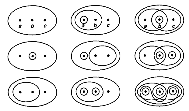
graphics grabbed from Munkres 75

Example

(discrete and co-discrete topology)

Let $S$ be any set. Then there are always the following two extreme possibilities of equipping $X$ with a topology $\tau \subset P(X)$ in the sense of def. , and hence making it a topological space:

1. $\tau \coloneqq P(S)$ the set of all open subsets;

   this is called the discrete topology on $S$, it is the finest topology (def. ) on $X$,

   we write $Disc(S)$ for the resulting topological space;

2. $\tau \coloneqq \{ \emptyset, S \}$ the set containing only the empty subset of $S$ and all of $S$ itself;

   this is called the codiscrete topology on $S$, it is the coarsest topology (def. ) on $X$,

   we write $CoDisc(S)$ for the resulting topological space.

The reason for this terminology is best seen when considering continuous functions into or out of these (co-)discrete topological spaces, we come to this in example below.

Example

(cofinite topology)

Given a set $X$, then the cofinite topology or finite complement topology on $X$ is the topology (def. ) whose open subsets are precisely

1. all cofinite subsets $S \subset X$ (i.e. those such that the complement $X \setminus S$ is a finite set);

2. the empty set.

If $X$ is itself a finite set (but not otherwise) then the cofinite topology on $X$ coincides with the discrete topology on $X$ (example ).

$\,$

We now consider basic construction principles of new topological spaces from given ones:

1. disjoint union spaces (example )

2. subspaces (example ),

3. quotient spaces (example )

4. product spaces (example ).

Below in Universal constructions we will recognize these as simple special cases of a general construction principle.

Example

(disjoint union space)

For $\{(X_i, \tau_i)\}_{i \in I}$ a set of topological spaces, then their disjoint union

$$\underset{i \in I}{\sqcup} (X_i, \tau_i)$$

is the topological space whose underlying set is the disjoint union of the underlying sets of the summand spaces, and whose open subsets are precisely the disjoint unions of the open subsets of the summand spaces.

In particular, for $I$ any index set, then the disjoint union of $I$ copies of the point space (example ) is equivalently the discrete topological space (example ) on that index set:

$$\underset{i \in I}{\sqcup} \ast \;=\; Disc(I) \,.$$

Example

(subspace topology)

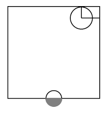
Let $(X, \tau_X)$ be a topological space, and let $S \subset X$ be a subset of the underlying set. Then the corresponding topological subspace has $S$ as its underlying set, and its open subsets are those subsets of $S$ which arise as restrictions of open subsets of $X$.

$$\left( U_S \subset S\,\,\text{open} \right) \,\Leftrightarrow\, \left( \underset{U_X \in \tau_X}{\exists} \left( U_S = U_X \cap S \right) \right) \,.$$

(This is also called the initial topology of the inclusion map. We come back to this below in def. .)

The picture on the right shows two open subsets inside the square, regarded as a topological subspace of the plane $\mathbb{R}^2$:

graphics grabbed from Munkres 75

Example

(quotient topological space)

Let $(X,\tau_X)$ be a topological space (def. ) and let

$$R_\sim \subset X \times X$$

be an equivalence relation on its underlying set. Then the quotient topological space has

• as underlying set the quotient set $X/\sim$, hence the set of equivalence classes,

and

• a subset $O \subset X/\sim$ is declared to be an open subset precisely if its preimage $\pi^{-1}(O)$ under the canonical projection map

  $$\pi \;\colon\; X \to X/\sim$$

  is open in $X$.

(This is also called the final topology of the projection $\pi$. We come back to this below in def. . )

Often one considers this with input datum not the equivalence relation, but any surjection

$$\pi \;\colon\; X \longrightarrow Y$$

of sets. Of course this identifies $Y = X/\sim$ with $(x_1 \sim x_2) \Leftrightarrow (\pi(x_1) = \pi(x_2))$. Hence the quotient topology on the codomain set of a function out of any topological space has as open subsets those whose pre-images are open.

To see that this indeed does define a topology on $X/\sim$ it is sufficient to observe that taking pre-images commutes with taking unions and with taking intersections.

Example

(binary product topological space)

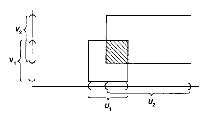
For $(X_1,\tau_{X_1})$ and $(X_2, \tau_{X_2})$ two topological spaces, then their binary product topological space has as underlying set the Cartesian product $X_1 \times X_2$ of the corresponding two underlying sets, and its topology is generated from the basis (def. ) given by the Cartesian products $U_1 \times U_2$ of the opens $U_i \in \tau_i$.

graphics grabbed from Munkres 75

Beware for non-finite products, the descriptions of the product topology is not as simple. This we turn to below in example , after introducing the general concept of limits in the category of topological spaces.

$\,$

The following examples illustrate how all these ingredients and construction principles may be combined.

The following example examines in more detail below in example , after we have introduced the concept of homeomorphisms below.

Example

Consider the real numbers $\mathbb{R}$ as the 1-dimensional Euclidean space (example ) and hence as a topological space via the corresponding metric topology (example ). Moreover, consider the closed interval $[0,1] \subset \mathbb{R}$ from example , regarded as a subspace (def. ) of $\mathbb{R}$.

The product space (example ) of this interval with itself

$$[0,1] \times [0,1]$$

is a topological space modelling the closed square. The quotient space (example ) of that by the relation which identifies a pair of opposite sides is a model for the cylinder. The further quotient by the relation that identifies the remaining pair of sides yields a model for the torus.

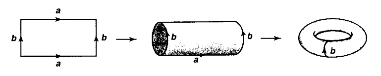
graphics grabbed from Munkres 75

Example

(spheres and disks)

For $n \in \mathbb{N}$ write

• $D^n$ for the n-disk, the closed unit ball (def. ) in the $n$-dimensional Euclidean space $\mathbb{R}^n$ (example ) and equipped with the induced subspace topology (example ) of the corresponding metric topology (example );

• $S^{n-1}$ for the (n-1)-sphere (def. ) also equipped with the corresponding subspace topology;

• $i_n \;\colon\; S^{n-1} \hookrightarrow D^n$ for the continuous function that exhibits this boundary inclusion.

Notice that

• $S^{-1} = \emptyset$ is the empty topological space (example );

• $S^0 = \ast \sqcup \ast$ is the disjoint union space (example ) of the point topological space (example ) with itself, equivalently the discrete topological space on two elements (example ).

The following important class of topological spaces form the foundation of algebraic geometry:

Example

(Zariski topology on affine space)

Let $k$ be a field, let $n \in \mathbb{N}$, and write $k[X_1, \cdots, X_n]$ for the set of polynomials in $n$ variables over $k$.

For $\mathcal{F} \subset k[X_1, \cdots, X_n]$ a subset of polynomials, let the subset $V(\mathcal{F}) \subset k^n$ of the $n$-fold Cartesian product of the underlying set of $k$ (the vanishing set of $\mathcal{F}$) be the subset of points on which all these polynomials jointly vanish:

$$V(\mathcal{F}) \coloneqq \left\{ (a_1, \cdots, a_n) \in k^n \,\vert\, \underset{f \in \mathcal{F}}{\forall} f(a_1, \cdots, a_n) = 0 \right\} \,.$$

These subsets are called the Zariski closed subsets.

Write

$$\tau_{\mathbb{A}^n_k} \;\coloneqq\; \left\{ k^n \setminus V(\mathcal{F}) \subset k^n \,\vert\, \mathcal{F} \subset k[X_1, \cdots, X_n] \right\}$$

for the set of complements of the Zariski closed subsets. These are called the Zariski open subsets of $k^n$.

The Zariski open subsets of $k^n$ form a topology (def. ), called the Zariski topology. The resulting topological space

$$\mathbb{A}^n_k \;\coloneqq\; \left( k^n, \tau_{\mathbb{A}^n_k} \right)$$

is also called the $n$-dimensional affine space over $k$.

More generally:

Example

(Zariski topology on the prime spectrum of a commutative ring)

Let $R$ be a commutative ring. Write $PrimeIdl(R)$ for its set of prime ideals. For $\mathcal{F} \subset R$ any subset of elements of the ring, consider the subsets of those prime ideals that contain $\mathcal{F}$:

$$V(\mathcal{F}) \;\coloneqq\; \left\{ p \in PrimeIdl(R) \,\vert\, \mathcal{F} \subset p \right\} \,.$$

These are called the Zariski closed subsets of $PrimeIdl(R)$. Their complements are called the Zariski open subsets.

Then the collection of Zariski open subsets in its set of prime ideals

$$\tau_{Spec(R)} \subset P(PrimeIdl(R))$$

satisfies the axioms of a topology (def. ), the Zariski topology.

This topological space

$$Spec(R) \coloneqq (PrimeIdl(R), \tau_{Spec(R)})$$

is called (the space underlying) the prime spectrum of the commutative ring.

$\,$

Closed subsets

The complements of open subsets in a topological space are called closed subsets (def. below). This simple definition indeed captures the concept of closure in the analytic sense of convergence of sequences (prop. below). Of particular interest for the theory of topological spaces in the discussion of separation axioms below are those closed subsets which are “irreducible” (def. below). These happen to be equivalently the “frame homomorphisms” (def. ) to the frame of opens of the point (prop. below).

Definition

(closed subsets)

Let $(X,\tau)$ be a topological space (def. ).

1. A subset $S \subset X$ is called a closed subset if its complement $X \setminus S$ is an open subset:

   $$\left( S \subset X\,\, \text{is closed} \right) \phantom{AA} \Leftrightarrow \phantom{AA} \left( X\setminus S \, \subset X \,\, \text{is open} \right) \,.$$

   graphics grabbed from Vickers 89

2. If a singleton subset $\{x\} \subset X$ is closed, one says that $x$ is a closed point of $X$.

3. Given any subset $S \subset X$, then its topological closure $Cl(S)$ is the smallest closed subset containing $S$:

   $$Cl(S) \;\coloneqq\; \underset{ {C \subset X\, \text{closed} } \atop {S \subset C } }{\cap} \left( C \right) \,.$$

4. A subset $S \subset X$ such that $Cl(S) = X$ is called a dense subset of $(X,\tau)$.

Often it is useful to reformulate def. of closed subsets as follows:

Lemma

(alternative characterization of topological closure)

Let $(X,\tau)$ be a topological space and let $S \subset X$ be a subset of its underlying set. Then a point $x \in X$ is contained in the topological closure $Cl(S)$ (def. ) precisely if every open neighbourhood $U_x \subset X$ of $x$ (def. ) intersects $S$:

$$\left( x \in Cl(S) \right) \phantom{AA} \Leftrightarrow \phantom{AA} \not\left( \underset{ {U \subset X \setminus S} \atop { U \subset X \, \text{open} } }{\exists} \left( x \in U \right) \right) \,.$$

Proof

Due to de Morgan duality (prop. ) we may rephrase the definition of the topological closure as follows:

$$\begin{aligned} Cl(S) & \coloneqq \underset{ {S \subset C } \atop { C \subset X\,\text{closed} } }{\cap} \left(C \right) \\ & = \underset{ { U \subset X \setminus S } \atop {U \subset X\, \text{open}} }{\cap} \left( X \setminus U \right) \\ & = X \setminus \left( \underset{ {U \subset X \setminus S} \atop { U \subset X\, \text{open} }}{\cup} U \right) \end{aligned} \,.$$

Proposition

(closure of a finite union is the union of the closures)

For $I$ a finite set and $\{U_i \subset X\}_{i \in I}$ a finite set of subsets of a topological space, we have

$$Cl(\underset{i \in I}{\cup}U_i) = \underset{i \in I}{\cup} Cl(U_i) \,.$$

Proof

By lemma we use that a point is in the closure of a set precisely if every open neighbourhood (def. ) of the point intersects the set.

Hence in one direction

$$\underset{i \in I}{\cup} Cl(U_i) \subset Cl(\underset{i \in I}{\cup}U_i)$$

because if every neighbourhood of a point intersects some $U_i$, then every neighbourhood intersects their union.

The other direction

$$Cl(\underset{i \in I}{\cup}U_i) \subset \underset{i \in I}{\cup} Cl(U_i)$$

is equivalent by de Morgan duality to

$$X \setminus \underset{i \in I}{\cup} Cl(U_i) \subset X \setminus Cl(\underset{i \in I}{\cup}U_i)$$

On left now we have the point for which there exists for each $i \in I$ a neighbourhood $U_{x,i}$ which does not intersect $U_i$. Since $I$ is finite, the intersection $\underset{i \in I}{\cap} U_{x,i}$ is still an open neighbourhood of $x$, and such that it intersects none of the $U_i$, hence such that it does not intersect their union. This implis that the given point is contained in the set on the right.

Definition

(topological interior and boundary)

Let $(X,\tau)$ be a topological space (def. ) and let $S \subset X$ be a subset. Then the topological interior of $S$ is the largest open subset $Int(S) \in \tau$ still contained in $S$, $Int(S) \subset S \subset X$:

$$Int(S) \coloneqq \underset{{O \subset S} \atop {O \subset X\, \text{open}}}{\cup} \left( U \right) \,.$$

The boundary $\partial S$ of $S$ is the complement of its interior inside its topological closure (def. ):

$$\partial S \;\coloneqq\; Cl(S) \setminus Int(S) \,.$$

Lemma

(duality between closure and interior)

Let $(X,\tau)$ be a topological space and let $S \subset X$ be a subset. Then the topological interior of $S$ (def. ) is the same as the complement of the topological closure $Cl(X\setminus S)$ of the complement of $S$:

$$X \setminus Int(S) \, = \, Cl(\, X \setminus S \,)$$

and conversely

$$X \setminus Cl(S) \, = \, Int(\, X \setminus S \,) \,.$$

Proof

Using de Morgan duality (prop. ), we compute as follows:

$$\begin{aligned} X \setminus Int(S) & = X \setminus \left( \underset{ {U \subset S} \atop {U \subset X \, open} }{\cup}U \right) \\ & = \underset{ {U \subset S} \atop {U \subset X \, \text{open}} }{\cap} \left( X \setminus U \right) \\ & = \underset{ {C \supset X \setminus S} \atop {C\, closed} }{\cap} \left( C \right) \\ & = Cl(X \setminus S) \end{aligned}$$

Similarly for the other case.

Example

(topological closure and interior of closed and open intervals)

Regard the real numbers as the 1-dimensional Euclidean space (example ) and equipped with the corresponding metric topology (example ) . Let $a \lt b \in \mathbb{R}$. Then the topological interior (def. ) of the closed interval $[a,b] \subset \mathbb{R}$ (example ) is the open interval $(a,b) \subset \mathbb{R}$, moreover the closed interval is its own topological closure (def. ) and the converse holds (by lemma ):

$$\array{ Cl\left( \,(a,b)\, \right) \,=\, [a,b] && Int\left( \, (a,b) \, \right) \,=\, (a,b) \\ \\ Cl\left( \,[a,b]\, \right) \,=\, [a,b] && Int\left(\,[a,b]\,\right) \,=\, (a,b) } \,.$$

Hence the boundary of the closed interval is its endpoints, while the boundary of the open interval is empty

$$\array{ \partial [a,b] = \{a\} \cup \{b\} && \partial(a,b) = \emptyset } \,.$$

The terminology “closed” subspace for complements of opens is justified by the following statement, which is a further example of how the combinatorial concept of open subsets captures key phenomena in analysis:

Proposition

(convergence in closed subspaces)

Let $(X,d)$ be a metric space (def. ), regarded as a topological space via example , and let $V \subset X$ be a subset. Then the following are equivalent:

1. $V \subset X$ is a closed subspace according to def. .

2. For every sequence $x_i \in V \subset X$ (def. ) with elements in $V$, which converges as a sequence in $X$ (def. ) to some $x_\infty \in X$, we have $x_\infty \in V \subset X$.

Proof

First assume that $V \subset X$ is closed and that $x_i \overset{i \to \infty}{\longrightarrow} x_{\infty}$ for some $x_\infty \in X$. We need to show that then $x_\infty \in V$. Suppose it were not, hence that $x_\infty \in X\setminus V$. Since, by assumption on $V$, this complement $X \setminus V \subset X$ is an open subset, it would follow that there exists a real number $\epsilon \gt 0$ such that the open ball around $x$ of radius $\epsilon$ were still contained in the complement: $B^\circ_x(\epsilon) \subset X \setminus V$. But since the sequence is assumed to converge in $X$, this would mean that there exists $N_\epsilon$ such that all $x_{i \gt N_{\epsilon}}$ are in $B^\circ_x(\epsilon)$, hence in $X\setminus V$. This contradicts the assumption that all $x_i$ are in $V$, and hence we have proved by contradiction that $x_\infty \in V$.

Conversely, assume that for all sequences in $V$ that converge to some $x_\infty \in X$ then $x_\infty \in V \subset X$. We need to show that then $V$ is closed, hence that $X \setminus V \subset X$ is an open subset, hence that for every $x \in X \setminus V$ we may find a real number $\epsilon \gt 0$ such that the open ball $B^\circ_x(\epsilon)$ around $x$ of radius $\epsilon$ is still contained in $X \setminus V$. Suppose on the contrary that such $\epsilon$ did not exist. This would mean that for each $k \in \mathbb{N}$ with $k \geq 1$ then the intersection $B^\circ_x(1/k) \cap V$ were non-empty. Hence then we could choose points $x_k \in B^\circ_x(1/k) \cap V$ in these intersections. These would form a sequence which clearly converges to the original $x$, and so by assumption we would conclude that $x \in V$, which violates the assumption that $x \in X \setminus V$. Hence we proved by contradiction $X \setminus V$ is in fact open.

Often one considers closed subsets inside a closed subspace. The following is immediate, but useful.

Lemma

(subsets are closed in a closed subspace precisely if they are closed in the ambient space)

Let $(X,\tau)$ be a topological space (def. ), and let $C \subset X$ be a closed subset (def. ), regarded as a topological subspace $(C,\tau_{sub})$ (example ). Then a subset $S \subset C$ is a closed subset of $(C,\tau_{sub})$ precisely if it is closed as a subset of $(X,\tau)$.

Proof

If $S \subset C$ is closed in $(C,\tau_{sub})$ this means equivalently that there is an open subset $V \subset C$ in $(C, \tau_{sub})$ such that

$$S = C \setminus V \,.$$

But by the definition of the subspace topology, this means equivalently that there is a subset $U \subset X$ which is open in $(X,\tau)$ such that $V = U \cap C$. Hence the above is equivalent to the existence of an open subset $U \subset X$ such that

$$\begin{aligned} S & = C \setminus V \\ & = C \setminus (U \cap C) \\ & = C \setminus U \end{aligned} \,.$$

But now the condition that $C$ itself is a closed subset of $(X,\tau)$ means equivalently that there is an open subset $W \subset X$ with $C = X \setminus W$. Hence the above is equivalent to the existence of two open subsets $W,U \subset X$ such that

$$S = (X \setminus W) \setminus U = X \setminus (W \cup U) \,.$$

Since the union $W \cup U$ is again open, this implies that $S$ is closed in $(X,\tau)$.

Conversely, that $S \subset X$ is closed in $(X,\tau)$ means that there exists an open $T \subset X$ with $S = X \setminus T \subset X$. This means that $S = S \cap C = (X \setminus T) \cap C = C\setminus T = C \setminus (T \cap C)$, and since $T \cap C$ is open in $(C,\tau_{sub})$ by definition of the subspace topology, this means that $S \subset C$ is closed in $(C, \tau_{sub})$.

A special role in the theory is played by the “irreducible” closed subspaces:

Definition

(irreducible closed subspace)

A closed subset $S \subset X$ (def. ) of a topological space $X$ is called irreducible if it is non-empty and not the union of two closed proper (i.e. smaller) subsets. In other words, a non-empty closed subset $S \subset X$ is irreducible if whenever $S_1, S_2 \subset X$ are two closed subspace such that

$$S = S_1 \cup S_2$$

then $S_1 = S$ or $S_2 = S$.

Example

(closures of points are irreducible)

For $x \in X$ a point inside a topological space, then the closure $Cl(\{x\})$ of the singleton subset $\{x\} \subset X$ is irreducible (def. ).

Example

(no nontrivial closed irreducibles in metric spaces)

Let $(X,d)$ be a metric space, regarded as a topological space via its metric topology (example ). Then every point $x \in X$ is closed (def ), hence every singleton subset $\{x\} \subset X$ is irreducible according to def. .

Let $\mathbb{R}$ be the 1-dimensional Euclidean space (example ) with its metric topology (example ). Then for $a \lt c \subset \mathbb{R}$ the closed interval $[a,c] \subset \mathbb{R}$ (example ) is not irreducible, since for any $b \in \mathbb{R}$ with $a \lt b \lt c$ it is the union of two smaller closed subintervals:

$$[a,c] \,=\, [a, b] \cup [b, c] \,.$$

In fact we will see below (prop. ) that in a metric space the singleton subsets are precisely the only irreducible closed subsets.

Often it is useful to re-express the condition of irreducibility of closed subspaces in terms of complementary open subsets:

Proposition

(irreducible closed subsets in terms of prime open subsets)

Let $(X, \tau)$ be a topological space, and let $P \in \tau$ be a proper open subset of $X$, hence so that the complement $F \coloneqq X\setminus P$ is a non-empty closed subspace. Then $F$ is irreducible in the sense of def. precisely if whenever $U_1,U_2 \in \tau$ are open subsets with $U_1 \cap U_2 \subset P$ then $U_1 \subset P$ or $U_2 \subset P$:

$$\left( X \setminus P \,\,\text{irreducible} \right) \;\Leftrightarrow\; \left( \underset{U_1, U_2 \in \tau}{\forall } \left( \left( U_1 \cap U_2 \subset P \right) \;\Rightarrow\; \left(U_1 \subset P \;\text{or}\; U_2 \subset P\right) \right) \right) \,.$$

The open subsets $P \subset X$ with this property are also called the prime open subsets in $\tau_X$.

Proof

Observe that every closed subset $F_i \subset F$ may be exhibited as the complement

$$F_i = F \setminus U_i$$

of some open subset $U_i \in \tau$ with respect to $F$. Observe that under this identification the condition that $U_1 \cap U_2 \subset P$ is equivalent to the condition that $F_1 \cup F_2 = F$, because it is equivalent to the equation labeled $(\star)$ in the following sequence of equations:

$$\begin{aligned} F_1 \cup F_2 & = (F \setminus U_1) \cup (F \setminus U_2) \\ & = \left( X \setminus (P \cup U_1) \right) \cup \left( X \setminus P \cup U_2 \right) \\ & = X \setminus \left( \left( P \cup U_1 \right) \cap \left( P \cup U_2 \right) \right) \\ & = X \setminus ( P \cup (U_1 \cap U_2) ) \\ & \stackrel{(\star)}{=} X \setminus P \\ & = F \,. \end{aligned} \,.$$

Similarly, the condition that $U_i \subset P$ is equivalent to the condition that $F_i = F$, because it is equivalent to the equality $(\star)$ in the following sequence of equalities:

$$\begin{aligned} F_i &= F \setminus U_i \\ & = X \setminus ( P \cup U_i ) \\ & \stackrel{(\star)}{=} X \setminus P \\ & = F \end{aligned} \,.$$

Under these identifications, the two conditions are manifestly the same.

We consider yet another equivalent characterization of irreducible closed subsets, prop. below, which will be needed in the discussion of the separation axioms further below. Stating this requires the following concept of “frame” homomorphism, the natural kind of homomorphisms between topological spaces if we were to forget the underlying set of points of a topological space, and only remember the set $\tau_X$ with its operations induced by taking finite intersections and arbitrary unions:

Definition

(frame homomorphisms)

Let $(X,\tau_X)$ and $(Y,\tau_Y)$ be topological spaces (def. ). Then a function

$$\tau_X \longleftarrow \tau_Y \;\colon\; \phi$$

between their sets of open subsets is called a frame homomorphism from $\tau_Y$ to $\tau_X$ if it preserves

1. arbitrary unions;

2. finiteintersections.

In other words, $\phi$ is a frame homomorphism precisely if

1. for every set $I$ and every $I$-indexed set $\{U_i \in \tau_Y\}_{i \in I}$ of elements of $\tau_Y$, then

   $$\phi\left(\underset{i \in I}{\cup} U_i\right) \;=\; \underset{i \in I}{\cup} \phi(U_i)\;\;\;\;\in \tau_X \,,$$

2. for every finite set $J$ and every $J$-indexed set $\{U_j \in \tau_Y\}_{j \in J}$ of elements in $\tau_Y$, then

   $$\phi\left(\underset{j \in J}{\cap} U_j\right) \;=\; \underset{j \in J}{\cap} \phi(U_j) \;\;\;\;\in \tau_X \,.$$

Remark

(frame homomorphisms preserve inclusions)

A frame homomorphism $\phi$ as in def. necessarily also preserves inclusions in that

• for every inclusion $U_1 \subset U_2$ with $U_1, U_2 \in \tau_Y \subset P(Y)$ then

  $$\phi(U_1) \subset \phi(U_2) \;\;\;\;\;\;\; \in \tau_X \,.$$

This is because inclusions are witnessed by unions

$$(U_1 \subset U_2) \;\Leftrightarrow\; \left( U_1 \cup U_2 = U_2 \right)$$

or alternatively because inclusions are witnessed by finite intersections:

$$(U_1 \subset U_2) \;\Leftrightarrow\; \left( U_1 \cap U_2 = U_1 \right) \,.$$

Example

(pre-images of continuous functions are frame homomorphisms)

Let $(X,\tau_X)$ and $(Y,\tau_Y)$ be two topological spaces. One way to obtain a function between their sets of open subsets

$$\tau_X \longleftarrow \tau_Y \;\colon\; \phi$$

is to specify a function

$$f \colon X \longrightarrow Y$$

of their underlying sets, and take $\phi \coloneqq f^{-1}$ to be the pre-image operation. A priori this is a function of the form

$$P(X) \longleftarrow P(Y) \;\colon\; f^{-1}$$

and hence in order for this to co-restrict to $\tau_X \subset P(X)$ when restricted to $\tau_Y \subset P(Y)$ we need to demand that, under $f$, pre-images of open subsets of $Y$ are open subsets of $Z$. Below in def. we highlight these as the continuous functions between topological spaces.

$$f \;\colon\; (X,\tau_X) \longrightarrow (Y, \tau_Y)$$

In this case then

$$\tau_X \longleftarrow \tau_Y \;\colon\; f^{-1}$$

is a frame homomorphism from $\tau_Y$ to $\tau_X$ in the sense of def. , by prop. .

For the following recall from example the point topological space $\ast = (\{1\}, \tau_\ast = \left\{\emptyset, \{1\}\right\})$.

Proposition

(irreducible closed subsets are equivalently frame homomorphisms to opens of the point)

For $(X,\tau)$ a topological space, then there is a natural bijection between the irreducible closed subspaces of $(X,\tau)$ (def. ) and the frame homomorphisms from $\tau_X$ to $\tau_\ast$, and this bijection is given by

$$\array{ FrameHom(\tau_X, \tau_\ast) &\underoverset{}{\simeq}{\longrightarrow}& IrrClSub(X) \\ \phi &\mapsto& X \setminus \left( U_\emptyset(\phi) \right) }$$

where $U_\emptyset(\phi)$ is the union of all elements $U \in \tau_x$ such that $\phi(U) = \emptyset$:

$$U_{\emptyset}(\phi) \coloneqq \underset{{U \in \tau_X} \atop {\phi(U) = \emptyset} }{\cup} \left( U \right) \,.$$

See also (Johnstone 82, II 1.3).

Proof

First we need to show that the function is well defined in that given a frame homomorphism $\phi \colon \tau_X \to \tau_\ast$ then $X \setminus U_\emptyset(\phi)$ is indeed an irreducible closed subspace.

To that end observe that:

$(\ast)$ If there are two elements $U_1, U_2 \in \tau_X$ with $U_1 \cap U_2 \subset U_{\emptyset}(\phi)$ then $U_1 \subset U_{\emptyset}(\phi)$ or $U_2 \subset U_{\emptyset}(\phi)$.

This is because

$$\begin{aligned} \phi(U_1) \cap \phi(U_2) & = \phi(U_1 \cap U_2) \\ & \subset \phi(U_{\emptyset}(\phi)) \\ & = \emptyset \end{aligned} \,,$$

where the first equality holds because $\phi$ preserves finite intersections by def. , the inclusion holds because $\phi$ respects inclusions by remark , and the second equality holds because $\phi$ preserves arbitrary unions by def. . But in $\tau_\ast = \{\emptyset, \{1\}\}$ the intersection of two open subsets is empty precisely if at least one of them is empty, hence $\phi(U_1) = \emptyset$ or $\phi(U_2) = \emptyset$. But this means that $U_1 \subset U_{\emptyset}(\phi)$ or $U_2 \subset U_{\emptyset}(\phi)$, as claimed.

Now according to prop. the condition $(\ast)$ identifies the complement $X \setminus U_{\emptyset}(\phi)$ as an irreducible closed subspace of $(X,\tau)$.

Conversely, given an irreducible closed subset $X \setminus U_0$, define $\phi$ by

$$\phi \;\colon\; U \mapsto \left\{ \array{ \emptyset & \vert \, \text{if} \, U \subset U_0 \\ \{1\} & \vert \, \text{otherwise} } \right. \,.$$

This does preserve

1. arbitrary unions

   because $\phi(\underset{i}{\cup} U_i) = \{\emptyset\}$ precisely if $\underset{i}{\cup}U_i \subset U_0$ which is the case precisely if all $U_i \subset U_0$, which means that all $\phi(U_i) = \emptyset$ and because $\underset{i}{\cup}\emptyset = \emptyset$;

   while $\phi(\underset{i}{\cup}U_1) = \{1\}$ as soon as one of the $U_i$ is not contained in $U_0$, which means that one of the $\phi(U_i) = \{1\}$ which means that $\underset{i}{\cup} \phi(U_i) = \{1\}$;

2. finite intersections

   because if $U_1 \cap U_2 \subset U_0$, then by $(\ast)$ $U_1 \subset U_0$ or $U_2 \subset U_0$, whence $\phi(U_1) = \emptyset$ or $\phi(U_2) = \emptyset$, whence with $\phi(U_1 \cap U_2) = \emptyset$ also $\phi(U_1) \cap \phi(U_2) = \emptyset$;

   while if $U_1 \cap U_2$ is not contained in $U_0$ then neither $U_1$ nor $U_2$ is contained in $U_0$ and hence with $\phi(U_1 \cap U_2) = \{1\}$ also $\phi(U_1) \cap \phi(U_2) = \{1\} \cap \{1\} = \{1\}$.

Hence this is indeed a frame homomorphism $\tau_X \to \tau_\ast$.

Finally, it is clear that these two operations are inverse to each other.

$\,$

Continuous functions

With the concept of topological spaces in hand (def. ) it is now immediate to formally implement in abstract generality the statement of prop. :

principle of continuity

$\,$ $\,$ Continuous pre-Images of open subsets are open.

Definition

(continuous function)

A continuous function between topological spaces (def. )

$$f \colon (X, \tau_X) \to (Y, \tau_Y)$$

is a function between the underlying sets,

$$f \colon X \longrightarrow Y$$

such that pre-images under $f$ of open subsets of $Y$ are open subsets of $X$.

We may equivalently state this in terms of closed subsets:

Proposition

Let $(X, \tau_X)$ and $(Y,\tau_Y)$ be two topological spaces (def. ). Then a function

$$f \;\colon\; X \longrightarrow Y$$

between the underlying sets is continuous in the sense of def. precisely if pre-images under $f$ of closed subsets of $Y$ (def. ) are closed subsets of $X$.

Proof

This follows since taking pre-images commutes with taking complements.

$\,$

Before looking at first examples of continuous functions below we consider now an informal remark on the resulting global structure, the “category of topological spaces”, remark below. This is a language that serves to make transparent key phenomena in topology which we encounter further below, such as the Tn-reflection (remark below), and the universal constructions.

Remark

(concrete category of topological spaces)

For $X_1, X_2, X_3$ three topological spaces and for

$$X_1 \overset{f}{\longrightarrow} X_2 \phantom{AA}\text{and}\phantom{AA} X_2 \overset{g}{\longrightarrow} X_3$$

two continuous functions (def. ) then their composition

$$f_2 \circ f_1 \;\colon\; X_1 \overset{f}{\longrightarrow} X_2 \overset{f_2}{\longrightarrow} X_3$$

is clearly itself again a continuous function from $X_1$ to $X_3$.

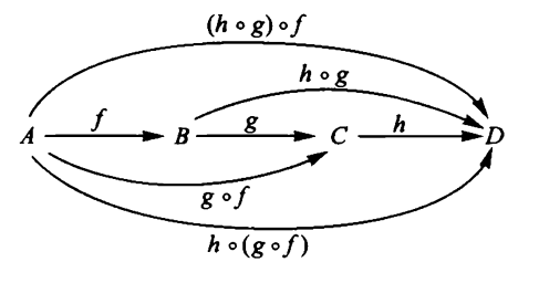
Moreover, this composition operation is clearly associative, in that for

$$X_1 \overset{f}{\longrightarrow} X_2 \phantom{AA}\text{and}\phantom{AA} X_2 \overset{g}{\longrightarrow} X_3 \phantom{AA}\text{and}\phantom{AA} X_3 \overset{h}{\longrightarrow} X_4$$

three continuous functions, then

$$f_3 \circ (f_2 \circ f_1) = (f_3 \circ f_2) \circ f_1 \;\colon\; X_1 \longrightarrow X_4 \,.$$

Finally, the composition operation is also clearly unital, in that for each topological space $X$ there exists the identity function $id_X \colon X \to X$ and for $f \colon X_1 \to X_2$ any continuous function then

$$id_{X_2} \circ f \;=\; f \;=\; f \circ id_{X_1} \,.$$

One summarizes this situation by saying that:

1. topological spaces constitute the objects,

2. continuous functions constitute the morphisms (homomorphisms)

of a category, called the category of topological spaces (“Top” for short).

It is useful to depict collections of objects with morphisms between them by diagrams, like this one:

$\,$

$\,$

$\,$

graphics grabbed from Lawvere-Schanuel 09.

There are other categories. For instance there is the category of sets (“Set” for short) whose

1. objects are sets,

2. morphisms are plain functions between these.

The two categories Top and Set are different, but related. After all,

1. an object of Top (hence a topological space) is an object of Set (hence a set) equipped with extra structure (namely with a topology);

2. a morphism in Top (hence a continuous function) is a morphism in Set (hence a plain function) with the extra property that it preserves this extra structure.

Hence we have the underlying set assigning function

$$\array{ Top &\overset{U}{\longrightarrow}& Set \\ \\ (X,\tau) &\overset{\phantom{AAa}}{\mapsto}& X }$$

from the class of topological spaces to the class of sets. But more is true: every continuous function between topological spaces is, by definition, in particular a function on underlying sets:

$$\array{ Top &\overset{U}{\longrightarrow}& Set \\ \\ (X,\tau_X) &\overset{\phantom{AAA}}{\mapsto}& X \\ {}^{\mathllap{f}}\downarrow &\overset{}{\mapsto}& \downarrow^{\mathrlap{f}} \\ (Y, \tau_Y) &\underset{\phantom{AAA}}{\mapsto}& Y }$$

and this assignment (trivially) respects the composition of morphisms and the identity morphisms.

Such a function between classes of objects of categories, which is extended to a function on the sets of homomorphisms between these objects in a way that respects composition and identity morphisms is called a functor. If we write an arrow between categories

$$U \;\colon\; Top \longrightarrow Set$$

then it is understood that we mean not just a function between their classes of objects, but a functor.

The functor $U$ at hand has the special property that it does not do much except forgetting extra structure, namely the extra structure on a set $X$ given by a choice of topology $\tau_X$. One also speaks of a forgetful functor.

This is intuitively clear, and we may easily formalize it: The functor $U$ has the special property that as a function between sets of homomorphisms (“hom sets”, for short) it is injective. More in detail, given topological spaces $(X,\tau_X)$ and $(Y,\tau_Y)$ then the component function of $U$ from the set of continuous function between these spaces to the set of plain functions between their underlying sets

$$\array{ \left\{ (X,\tau_X) \underoverset{\text{function}}{\text{continuous}}{\longrightarrow} (Y,\tau_Y) \right\} &\;\overset{\phantom{AA}U\phantom{AA}}{\mapsto}\;& \left\{ X \underset{\text{function}}{\longrightarrow} Y \right\} }$$

is an injective function, including the continuous functions among all functions of underlying sets.

A functor with this property, that its component functions between all hom-sets are injective, is called a faithful functor.

A category equipped with a faithful functor to Set is called a concrete category.

Hence Top is canonically a concrete category.

Example

(product topological space construction is functorial)

For $\mathcal{C}$ and $\mathcal{D}$ two categories as in remark (for instance Top or Set) then we obtain a new category denoted $\mathcal{C} \times \mathcal{D}$ and called their product category whose

1. objects are pairs $(c,d)$ with $c$ an object of $\mathcal{C}$ and $d$ an object of $\mathcal{D}$;

• morphisms are pairs $(f,g) \;\colon\; (c,d) \to (c', d')$ with $f \colon c \to c'$ a morphism of $\mathcal{C}$

  and $g \colon d \to d'$ a morphism of $\mathcal{D}$,

• composition of morphisms is defined pairwise $(f', g') \circ (f,g) \coloneqq ( f' \circ f, g' \circ g )$.

This concept secretly underlies the construction of product topological spaces:

Let $(X_1,\tau_{X_1})$, $(X_2, \tau_{X_2})$, $(Y_1, \tau_{Y_1})$ and $(Y_2, \tau_{Y_2})$ be topological spaces. Then for all pairs of continuous functions

$$f_1 \;\colon\; (X_1, \tau_{X_1}) \longrightarrow (Y_1, \tau_{Y_1})$$

and

$$f_2 \;\colon\; (X_2, \tau_{X_2}) \longrightarrow (Y_2, \tau_{Y_2})$$

the canonically induced function on Cartesian products of sets

$$\array{ X_1 \times X_2 & \overset{ f_1 \times f_2 }{\longrightarrow} & Y_1 \times Y_2 \\ (x_1, x_2) &\mapsto& ( f_1(x_1), f_2(x_2) ) }$$

is clearly a continuous function with respect to the binary product space topologies (def. )

$$f_1 \times f_2 \;\colon\; (X_1 \times X_2, \tau_{X_1 \times X_2}) \longrightarrow (Y_1 \times Y_2, \tau_{Y_1 \times Y_2}) \,.$$

Moreover, this construction respects identity functions and composition of functions in both arguments.

In the language of category theory (remark ), this is summarized by saying that the product topological space construction $(-) \times (-)$ extends to a functor from the product category of the category Top with itself to itself:

$$(-) \times (-) \;\colon\; Top \times Top \longrightarrow Top \,.$$

$\,$

Examples

We discuss here some basic examples of continuous functions (def. ) between topological spaces (def. ) to get a feeling for the nature of the concept. But as with topological spaces themselves, continuous functions between them are ubiquitous in mathematics, and no list will exhaust all classes of examples. Below in the section Universal constructions we discuss a general principle that serves to produce examples of continuous functions with prescribed “universal properties”.

Example

(point space is terminal)

For $(X,\tau)$ any topological space, then there is a unique continuous function

1. from the empty topological space (def. ) $X$

   $$\emptyset \overset{\phantom{AA} \exists ! \phantom{AA} }{\longrightarrow} X$$

2. from $X$ to the point topological space (def. ).

   $$X \overset{\phantom{AA} \exists ! \phantom{AA}}{\longrightarrow} \ast$$

In the language of category theory (remark ), this says that

1. the empty topological space is the initial object

2. the point space $\ast$ is the terminal object

in the category Top of topological spaces. We come back to this below in example .

Example

(constant continuous functions)

For $(X, \tau)$ a topological space then for $x \in X$ any element of the underlying set, there is a unique continuous function (which we denote by the same symbol)

$$x \;\colon\; \ast \longrightarrow X$$

from the point topological space (def. ), whose image in $X$ is that element. Hence there is a natural bijection

$$\left\{ \ast \overset{f}{\to} X \,\vert\, f \,\,\text{continuous} \right\} \;\simeq\; X$$

between the continuous functions from the point to any topological space, and the underlying set of that topological space.

More generally, for $(X,\tau_X)$ and $(Y,\tau_Y)$ two topological spaces, then a continuous function $X \to Y$ between them is called a constant function with value some point $y \in Y$ if it factors through the point spaces as

$$const_y \;\colon\; X \overset{\exists !}{\longrightarrow} \ast \overset{y}{\longrightarrow} Y \,.$$

Definition

(locally constant function)

For $(X,\tau_X)$, $(Y,\tau_Y)$ two topological spaces, then a continuous function $f \colon (X,\tau_X) \to (Y,\tau_Y)$ (def. ) is called locally constant if every point $x \in X$ has a neighbourhood (def. ) on which the function is constant.

Example

(continuous functions into and out of discrete and codiscrete spaces)

Let $S$ be a set and let $(X,\tau)$ be a topological space. Recall from example

1. the discrete topological space $Disc(S)$;

2. the co-discrete topological space $CoDisc(S)$

on the underlying set $S$. Then continuous functions (def. ) into/out of these satisfy:

1. every function (of sets) $Disc(S) \longrightarrow X$ out of a discrete space is continuous;

2. every function (of sets) $X \longrightarrow CoDisc(S)$ into a codiscrete space is continuous.

Also:

• every continuous function $(X,\tau) \longrightarrow Disc(S)$ into a discrete space is locally constant (def. ).

Example

(diagonal)

For $X$ a set, its diagonal $\Delta_X$ is the function from $X$ to the Cartesian product of $X$ with itself, given by

$$\array{ X &\overset{\Delta_X}{\longrightarrow}& X \times X \\ x &\mapsto& (x,x) }$$

For $(X,\tau)$ a topological space, then the diagonal is a continuous function to the product topological space (def. ) of $X$ with itself.

$$\Delta_X \;\colon\; (X, \tau) \longrightarrow (X \times X, \tau_{X \times X}) \,.$$

To see this, it is sufficient to see that the preimages of basic opens $U_1 \times U_2$ in $\tau_{X \times X}$ are in $\tau_X$. But these pre-images are the intersections $U_1 \cap U_2 \subset X$, which are open by the axioms on the topology $\tau_X$.

Example

(image factorization)

Let $f \;\colon\; (X, \tau_X) \longrightarrow (Y,\tau_Y)$ be a continuous function.

Write $f(X) \subset Y$ for the image of $f$ on underlying sets, and consider the resulting factorization of $f$ through $f(X)$ on underlying sets:

$$f \;\colon\; X \overset{\text{surjective}}{\longrightarrow} f(X) \overset{\text{injective}}{\longrightarrow} Y \,.$$

There are the following two ways to topologize the image $f(X)$ such as to make this a sequence of two continuous functions:

1. By example $f(X)$ inherits a subspace topology from $(Y,\tau_Y)$ which evidently makes the inclusion $f(X) \longrightarrow Y$ a continuous function.

   Observe that this also makes $X \to f(X)$ a continuous function: An open subset of $f(X)$ in this case is of the form $U_Y \cap f(X)$ for $U_Y \in \tau_Y$, and $f^{-1}( U_Y \cap f(X) ) = f^{-1}(U_Y)$, which is open in $X$ since $f$ is continuous.

2. By example $f(X)$ inherits a quotient topology from $(X,\tau_X)$ which evidently makes the surjection $X \longrightarrow f(X)$ a continuous function.

   Observe that this also makes $f(X) \longrightarrow Y$ a continuous function: The preimage under this map of an open subset $U_Y \in \tau_Y$ is the restriction $U_Y \cap f(X)$, and the pre-image of that under $X \to f(X)$ is $f^{-1}(U_Y)$, as before, which is open since $f$ is continuous, and therefore $U_Y \cap f(X)$ is open in the quotient topology.

$\,$

Beware, in general a continuous function itself (as opposed to its pre-image function) neither preserves open subsets, nor closed subsets, as the following examples show:

Example

Regard the real numbers $\mathbb{R}$ as the 1-dimensional Euclidean space (example ) equipped with the metric topology (example ). For $a \in \mathbb{R}$ the constant function (example )

$$\array{ \mathbb{R} &\overset{const_a}{\longrightarrow}& \mathbb{R} \\ x &\mapsto& a }$$

maps every open subset $U \subset \mathbb{R}$ to the singleton set $\{a\} \subset \mathbb{R}$, which is not open.

Example

Write $Disc(\mathbb{R})$ for the set of real numbers equipped with its discrete topology (def. ) and $\mathbb{R}$ for the set of real numbers equipped with its Euclidean metric topology (example , example ). Then the identity function on the underlying sets

$$id_{\mathbb{R}} \;\colon\; Disc(\mathbb{R}) \longrightarrow \mathbb{R}$$

is a continuous function (a special case of example ). A singleton subset $\{a\} \in Disc(\mathbb{R})$ is open, but regarded as a subset $\{a\} \in \mathbb{R}$ it is not open.

Example

Consider the set of real numbers $\mathbb{R}$ equipped with its Euclidean metric topology (example , example ). The exponential function

$$\exp(-) \;\colon\; \mathbb{R} \longrightarrow \mathbb{R}$$

maps all of $\mathbb{R}$ (which is a closed subset, since $\mathbb{R} = \mathbb{R} \setminus \emptyset$) to the open interval $(0,\infty) \subset \mathbb{R}$, which is not closed.

Those continuous functions that do happen to preserve open or closed subsets get a special name:

Definition

(open maps and closed maps)

A continuous function $f \colon (X,\tau_X) \to (Y, \tau_Y)$ (def. ) is called

• an open map if the image under $f$ of an open subset of $X$ is an open subset of $Y$;

• a closed map if the image under $f$ of a closed subset of $X$ (def. ) is a closed subset of $Y$.

Example

(image projections of open/closed maps are themselves open/closed)

If a continuous function $f \colon (X,\tau_X) \to (Y,\tau_Y)$ is an open map or closed map (def. ) then so its its image projection $X \to f(X) \subset Y$, respectively, for $f(X) \subset Y$ regarded with its subspace topology (example ).

Proof

If $f$ is an open map, and $O \subset X$ is an open subset, so that $f(O) \subset Y$ is also open in $Y$, then, since $f(O) = f(O) \cap f(X)$, it is also still open in the subspace topology, hence $X \to f(X)$ is an open map.

If $f$ is a closed map, and $C \subset X$ is a closed subset so that also $f(C) \subset Y$ is a closed subset, then the complement $Y \setminus f(C)$ is open in $Y$ and hence $(Y \setminus f(C)) \cap f(X) = f(X) \setminus f(C)$ is open in the subspace topology, which means that $f(C)$ is closed in the subspace topology.

Example

(projections are open continuous functions )

For $(X_1,\tau_{X_1})$ and $(X_2,\tau_{X_2})$ two topological spaces, then the projection maps

$$pr_i \;\colon\; (X_1 \times X_2, \tau_{X_1 \times X_2}) \longrightarrow (X_i, \tau_{X_i})$$

out of their product topological space (def. )

$$\array{ X_1 \times X_2 &\overset{pr_1}{\longrightarrow}& X_1 \\ (x_1, x_2) &\overset{\phantom{AAA}}{\mapsto}& x_1 }$$

$$\array{ X_1 \times X_2 &\overset{pr_2}{\longrightarrow}& X_2 \\ (x_1, x_2) &\overset{\phantom{AAA}}{\mapsto}& x_2 }$$

are open continuous functions (def. ).

This is because, by definition, every open subset $O \subset X_1 \times X_2$ in the product space topology is a union of products of open subsets $U_i \in X_1$ and $V_i \in X_2$ in the factor spaces

$$O = \underset{i \in I}{\cup} \left( U_i \times V_i \right)$$

and because taking the image of a function preserves unions of subsets

$$\begin{aligned} pr_1\left( \underset{i \in I}{\cup} \left( U_i \times V_i \right) \right) & = \underset{i \in I}{\cup} pr_1 \left( U_i \times V_i \right) \\ & = \underset{i \in I}{\cup} U_i \end{aligned} \,.$$

Below in prop. we find a large supply of closed maps.

$\,$

Sometimes it is useful to recognize quotient topological space projections via saturated subsets (essentially another term for pre-images of underlying sets):

Definition

(saturated subset)

Let $f \;\colon\; X \longrightarrow Y$ be a function of sets. Then a subset $S \subset X$ is called an $f$-saturated subset (or just saturated subset, if $f$ is understood) if $S$ is the pre-image of its image:

$$\left(S \subset X \,\, f\text{-saturated} \right) \,\Leftrightarrow\, \left( S = f^{-1}(f(S)) \right) \,.$$

Here $f^{-1}(f(S))$ is also called the $f$-saturation of $S$.

Example

(pre-images are saturated subsets)

For $f \;\colon\; X \to Y$ any function of sets, and $S_Y \subset Y$ any subset of $Y$, then the pre-image $f^{-1}(S_Y) \subset X$ is an $f$-saturated subset of $X$ (def. ).

Observe that:

Lemma

Let $f \colon X \longrightarrow Y$ be a function. Then a subset $S \subset X$ is $f$-saturated (def. ) precisely if its complement $X \setminus S$ is saturated.

Proposition

(recognition of quotient topologies)

A continuous function (def. )

$$f \;\colon\; (X, \tau_X) \longrightarrow (Y,\tau_Y)$$

whose underlying function $f \colon X \longrightarrow Y$ is surjective exhibits $\tau_Y$ as the corresponding quotient topology (def. ) precisely if $f$ sends open and $f$-saturated subsets in $X$ (def. ) to open subsets of $Y$. By lemma this is the case precisely if it sends closed and $f$-saturated subsets to closed subsets.

We record the following technical lemma about saturated subspaces, which we will need below to prove prop. .

Lemma

(saturated open neighbourhoods of saturated closed subsets under closed maps)

Let

1. $f \;\colon\; (X, \tau_X) \longrightarrow (Y, \tau_Y)$ be a closed map (def. );

2. $C \subset X$ be a closed subset of $X$ (def. ) which is $f$-saturated (def. );

3. $U \supset C$ be an open subset containing $C$;

then there exists a smaller open subset $V$ still containing $C$

$$U \supset V \supset C$$

and such that $V$ is still $f$-saturated.

Proof

We claim that the complement of $X$ by the $f$-saturation (def. ) of the complement of $X$ by $U$

$$V \coloneqq X \setminus \left( f^{-1}\left( f\left( X \setminus U \right) \right) \right)$$

has the desired properties. To see this, observe first that

1. the complement $X \setminus U$ is closed, since $U$ is assumed to be open;

2. hence the image $f(X\setminus U)$ is closed, since $f$ is assumed to be a closed map;

3. hence the pre-image $f^{-1}\left( f\left( X \setminus U \right)\right)$ is closed, since $f$ is continuous (using prop. ), therefore its complement $V$ is indeed open;

4. this pre-image $f^{-1}\left( f\left( X \setminus U \right) \right)$ is saturated (by example ) and hence also its complement $V$ is saturated (by lemma ).

Therefore it now only remains to see that $U \supset V \supset C$.

By de Morgan's law (prop. ) the inclusion $U \supset V$ is equivalent to the inclusion $f^{-1}\left( f\left( X \setminus U \right)\right) \supset X \setminus U$, which is clearly the case.

The inclusion $V \supset C$ is equivalent to $f^{-1}\left( f\left( X \setminus U \right) \right) \,\cap \, C = \emptyset$. Since $C$ is saturated by assumption, this is equivalent to $f^{-1}\left( f\left( X \setminus U \right)\right) \,\cap \, f^{-1}(f(C)) = \emptyset$. This in turn holds precisely if $f\left( X \setminus U \right) \,\cap \, f(C) = \emptyset$. Since $C$ is saturated, this holds precisely if $X \setminus U \cap C = \emptyset$, and this is true by the assumption that $U \supset C$.

$\,$

Homeomorphisms

With the objects (topological spaces) and the morphisms (continuous functions) of the category Top thus defined (remark ), we obtain the concept of “sameness” in topology. To make this precise, one says that a morphism

$$X \overset{f}{\to} Y$$

in a category is an isomorphism if there exists a morphism going the other way around

$$X \overset{g}{\longleftarrow} Y$$

which is an inverse in the sense that both its compositions with $f$ yield an identity morphism:

$$f \circ g = id_Y \;\;\;\;\; and \;\;\;\;\; g \circ f = id_X \,.$$

Since such $g$ is unique if it exists, one often writes “$f^{-1}$” for this inverse morphism.

Definition

(homeomorphisms)

An isomorphism in the category Top (remark ) of topological spaces (def. ) with continuous functions between them (def. ) is called a homeomorphism.

Hence a homeomorphism is a continuous function

$$f \;\colon\; (X, \tau_X) \longrightarrow (Y, \tau_Y)$$

between two topological spaces $(X,\tau_X)$, $(Y,\tau_Y)$ such that there exists another continuous function the other way around

$$(X, \tau_X) \longleftarrow (Y, \tau_Y) \;\colon\; g$$

such that their composites are the identity functions on $X$ and $Y$, respectively:

$$f \circ g = id_{Y} \;\;\;and\;\;\; g \circ f = id_{X} \,.$$

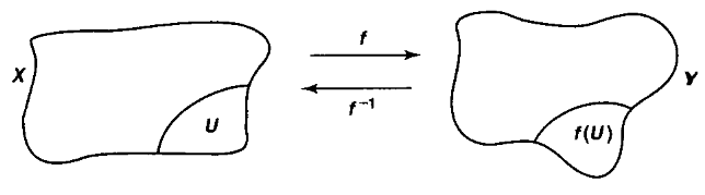
graphics grabbed from Munkres 75

We notationally indicate that a continuous function is a homeomorphism by the symbol “$\simeq$”.

$$f \;\colon\; (X,\tau_X) \overset{\simeq}{\longrightarrow} (Y,\tau_Y) \,.$$

If there is some, possibly unspecified, homeomorphism between topological spaces $(X,\tau_X)$ and $(Y,\tau_Y)$, then we also write

$$(X,\tau_X) \,\simeq\, (Y,\tau_Y)$$

and say that the two topological spaces are homeomorphic.

A property/predicate $P$ of topological spaces which is invariant under homeomorphism in that

$$\left( (X, \tau_X) \, \simeq \, (Y,\tau_Y) \right) \;\Rightarrow\; \left( P(X,\tau_X) \,\Leftrightarrow\, P(Y,\tau_Y) \right)$$

is called a topological property or topological invariant.

Remark

(notation for homeomorphisms)

Beware the following notation:

1. In topology the notation $f^{-1}$ generally refers to the pre-image function of a given function $f$, while if $f$ is a homeomorphism (def. ), it is also used for the inverse function of $f$. This abuse of notation is convenient: If $f$ happens to be a homeomorphism, then the pre-image of a subsets under $f$ is its image under the inverse function $f^{-1}$.

2. Many authors strictly distinguish the symbols “$\cong$” and “$\simeq$” and use the former to denote homeomorphisms and the latter to refer to homotopy equivalences (which we consider in part 2). We use either symbol (but mostly “$\simeq$”) for “isomorphism” in whatever the ambient category may be and try to make that context always unambiguously explicit.

Remark

If $f \colon (X, \tau_X) \to (Y, \tau_Y)$ is a homeomorphism (def. ) with inverse continuous function $g$, then

1. also $g$ is a homeomophism, with inverse continuous function $f$;

2. the underlying function of sets $f \colon X \to Y$ of a homeomorphism $f$ is necessarily a bijection, with inverse bijection $g$.

But beware that not every continuous function which is bijective on underlying sets is a homeomorphism. While an inverse function $g$ will exists on the level of functions of sets, this inverse may fail to be continuous:

Counter Example

Consider the continuous function

$$\array{ [0,2\pi) &\longrightarrow& S^1 \subset \mathbb{R}^2 \\ t &\mapsto& (cos(t), sin(t)) }$$

from the half-open interval (def. ) to the unit circle $S^1 \coloneqq S_0(1) \subset \mathbb{R}^2$ (def. ), regarded as a topological subspace (example ) of the Euclidean plane (example ).

The underlying function of sets of $f$ is a bijection. The inverse function of sets however fails to be continuous at $(1,0) \in S^1 \subset \mathbb{R}^2$. Hence this $f$ is not a homeomorphism.

Indeed, below we see that the two topological spaces $[0,2\pi)$ and $S^1$ are distinguished by topological invariants, meaning that they cannot be homeomorphic via any (other) choice of homeomorphism. For example $S^1$ is a compact topological space (def. ) while $[0,2\pi)$ is not, and $S^1$ has a non-trivial fundamental group, while that of $[0,2\pi)$ is trivial (this prop.).

Below in example we discuss a practical criterion under which continuous bijections are homeomorphisms after all. But immediate from the definitions is the following characterization:

Proposition

(homeomorphisms are the continuous and open bijections)

Let $f \;\colon\; (X, \tau_X) \longrightarrow (Y,\tau_Y)$ be a continuous function between topological spaces (def. ). Then the following are equivalence:

1. $f$ is a homeomorphism;

2. $f$ is a bijection and an open map (def. );

3. $f$ is a bijection and a closed map (def. ).

Proof

It is clear from the definition that a homeomorphism in particular has to be a bijection. The condition that the inverse function $Y \leftarrow X \colon g$ be continuous means that the pre-image function of $g$ sends open subsets to open subsets. But by $g$ being the inverse to $f$, that pre-image function is equal to $f$, regarded as a function on subsets:

$$g^{-1} = f \;\colon\; P(X) \to P(Y) \,.$$

Hence $g^{-1}$ sends opens to opens precisely if $f$ does, which is the case precisely if $f$ is an open map, by definition. This shows the equivalence of the first two items. The equivalence between the first and the third follows similarly via prop. .

$\,$

Now we consider some actual examples of homeomorphisms:

Example

(concrete point homeomorphic to abstract point space)

Let $(X,\tau_X)$ be a non-empty topological space, and let $x \in X$ be any point. Regard the corresponding singleton subset $\{x\} \subset X$ as equipped with its subspace topology $\tau_{\{x\}}$ (example ). Then this is homeomorphic (def. ) to the abstract point space from example :

$$(\{x\}, \tau_{\{x\}} ) \,\simeq\, \ast \,.$$

Example

(open interval homeomorphic to the real line)

Regard the real line as the 1-dimensional Euclidean space (example ) with its metric topology (example ).

Then the open interval $(-1,1) \subset \mathbb{R}$ (def. ) regarded with its subspace topology (example ) is homeomorphic (def.) to all of the real line

$$(-1,1) \,\simeq\, \mathbb{R}^1 \,.$$

An inverse pair of continuous functions is for instance given (via example ) by

$$\array{ f &\colon& \mathbb{R}^1 &\longrightarrow& (-1,+1) \\ && x &\mapsto& \frac{x}{\sqrt{1+ x^2}} }$$

and

$$\array{ g &\colon& (-1,+1) &\longrightarrow& \mathbb{R}^1 \\ && x &\mapsto& \frac{x}{\sqrt{1 - x^2}} } \,.$$

But there are many other choices for $f$ and $g$ that yield a homeomorphism.

Similarly, for all $a \lt b \in \mathbb{R}$

1. the open intervals $(a,b) \subset \mathbb{R}$ (example ) equipped with their subspace topology are all homeomorphic to each other,

2. the closed intervals $[a,b]$ are all homeomorphic to each other,

3. the half-open intervals of the form $[a,b)$ are all homeomorphic to each other;

4. the half-open intervals of the form $(a,b]$ are all homeomorphic to each other.

Generally, every open ball in $\mathbb{R}^n$ (def. ) is homeomorphic to all of $\mathbb{R}^n$:

$$\left( B^\circ_0(\epsilon) \subset \mathbb{R}^n \right) \,\simeq\, \mathbb{R}^n \,.$$

While mostly the interest in a given homeomorphism is in it being non-obvious from the definitions, many homeomorphisms that appear in practice exhibit “obvious re-identifications” for which it is of interest to leave them consistently implicit:

Example

(homeomorphisms between iterated product spaces)

Let $(X,\tau_X)$, $(Y,\tau_Y)$ and $(Z, \tau_Z)$ be topological spaces.

Then:

1. There is an evident homeomorphism between the two ways of bracketing the three factors when forming their product topological space (def. ), called the associator:

   $$\alpha_{X,Y,Z} \;\colon\; \left( (X, \tau_X) \times (Y, \tau_Y) \right) \times (Z, \tau_Z) \overset{\phantom{AA}\simeq\phantom{AA}}{\longrightarrow} (X,\tau_X) \times \left( (Y,\tau_Y) \times (Z, \tau_Z) \right) \,.$$

2. There are evident homeomorphism between $(X,\tau)$ and its product topological space (def. ) with the point space $\ast$ (example ), called the left and right unitors:

   $$\lambda_X \;\colon\; \ast \times (X, \tau_X) \overset{\phantom{AA}\simeq\phantom{AA}}{\longrightarrow} (X,\tau_X)$$

   and

   $$\rho_X \;\colon\; (X, \tau_X) \times \ast \overset{\phantom{AA}\simeq\phantom{AA}}{\longrightarrow} (X, \tau_X) \,.$$

3. There is an evident homeomorphism between the results of the two orders in which to form their product topological spaces (def. ), called the braiding:

   $$\beta_{X,Y} \;\colon\; (X,\tau_X) \times (Y,\tau_Y) \overset{\phantom{AA}\simeq\phantom{AA}}{\longrightarrow} (Y,\tau_Y) \times (X, \tau_X) \,.$$

Moreover, all these homeomorphisms are compatible with each other, in that they make the following diagrams commute (recall remark ):

1. (triangle identity)

   $$\array{ & (X \times \ast ) \times Y &\stackrel{\alpha_{X,\ast,Y}}{\longrightarrow} & X \times (\ast \times Y) \\ & {}_{\rho_x \times id_Y}\searrow && \swarrow_{id_X \times \lambda_Y} & \\ && X \times Y }$$

2. (pentagon identity)

   $$\array{ && (W \times X) \times (Y \times Z) \\ & {}^{\mathllap{\alpha_{W \times X, Y, Z}}}\nearrow && \searrow^{\mathrlap{\alpha_{W,X,Y \times Z}}} \\ ((W \times X ) \times Y) \times Z && && (W \times (X \times (Y \times Z))) \\ {}^{\mathllap{\alpha_{W,X,Y}} \times id_Z }\downarrow && && \uparrow^{\mathrlap{ id_W \times \alpha_{X,Y,Z} }} \\ (W \times (X \times Y)) \times Z && \underset{\alpha_{W,X \times Y, Z}}{\longrightarrow} && W \times ( (X \times Y) \times Z ) }$$

3. (hexagon identities)

   $$\array{ (X \times Y) \times Z &\stackrel{\alpha_{X,Y,Z}}{\longrightarrow}& X \times (Y \times Z) &\stackrel{\beta_{X,Y \times Z}}{\longrightarrow}& (Y \times Z) \times X \\ \downarrow^{\beta_{X,Y} \times id_Z} &&&& \downarrow^{\alpha_{Y,Z,X}} \\ (Y \times X) \times Z &\stackrel{\alpha_{Y,X,Z}}{\longrightarrow}& Y \times (X \times Z) &\stackrel{id_Y \times \beta_{X,Y}}{\longrightarrow}& Y \times (Z \times X) }$$

   and

   $$\array{ X \times (Y \times Z) &\stackrel{\alpha^{inv}_{X,Y,Z}}{\longrightarrow}& (X \times Y) \times Z &\stackrel{\beta_{X \times Y, Z}}{\longrightarrow}& Z \times (X \times Y) \\ \downarrow^{id_X \times \beta_{Y,Z}} &&&& \downarrow^{\alpha^{inv}_{Z,X,Y}} \\ X \times (Z \times Y) &\stackrel{\alpha^{inv}_{X,Z,Y}}{\longrightarrow}& (X \times Z) \times Y &\stackrel{\beta_{X,Z} \times id}{\longrightarrow}& (Z \times X) \times Y } \,,$$

4. (symmetry)

   $$\beta_{Y,X} \circ \beta_{X,Y} \;=\; id \;\colon\; (X_1 \times X_2 \tau_{X_1 \times X_2}) \to (X_1 \times X_2 \tau_{X_1 \times X_2}) \,.$$

In the language of category theory (remark ), all this is summarized by saying that the the functorial construction $(-) \times (-)$ of product topological spaces (example ) gives the category Top of topological spaces the structure of a monoidal category which moreover is symmetrically braided.

From this, a basic result of category theory, the MacLane coherence theorem, guarantees that there is no essential ambiguity re-backeting arbitrary iterations of the binary product topological space construction, as long as the above homeomorphisms are understood.

Accordingly, we may write

$$(X_1, \tau_1) \times (X_2, \tau_2) \times \cdots \times (X_n, \tau_n)$$

for iterated product topological spaces without putting parenthesis.

$\,$

The following are a sequence of examples all of the form that an abstractly constructed topological space is homeomorphic to a certain subspace of a Euclidean space. These examples are going to be useful in further developments below, for example in the proof below of the Heine-Borel theorem (prop. ).

• Products of intervals are homeomorphic to hypercubes (example ).

• The closed interval glued at its endpoints is homeomorphic to the circle (example ).

• The cylinder, the Möbius strip and the torus are all homeomorphic to quotients of the square (example ).

Example

(product of closed intervals homeomorphic to hypercubes)

Let $n \in \mathbb{N}$, and let $[a_i, b_i] \subset \mathbb{R}$ for $i \in \{1, \cdots, n\}$ be $n$ closed intervals in the real line (example ), regarded as topological subspaces of the 1-dimensional Euclidean space (example ) with its metric topology (example ). Then the product topological space (def. , example ) of all these intervals is homeomorphic (def. ) to the corresponding topological subspace of the $n$-dimensional Euclidean space (example ):

$$[a_1, b_1] \times [a_2, b_2] \times \cdots \times [a_n, b_n] \;\simeq\; \left\{ \vec x \in \mathbb{R}^n \,\vert\, \underset{i}{\forall} (a_i \leq x_i \leq b_i) \right\} \subset \mathbb{R}^n \,.$$

Similarly for open intervals:

$$(a_1, b_1) \times (a_2, b_2) \times \cdots \times (a_n, b_n) \;\simeq\; \left\{ \vec x \in \mathbb{R}^n \,\vert\, \underset{i}{\forall} (a_i \lt x_i \lt b_i) \right\} \subset \mathbb{R}^n \,.$$

Proof

There is a canonical bijection between the underlying sets. It remains to see that this, as well and its inverse, are continuous functions. For this it is sufficient to see that under this bijection the defining basis (def. ) for the product topology is also a basis for the subspace topology. But this is immediate from lemma .

Example

(closed interval glued at endpoints homeomorphic circle)

As topological spaces, the closed interval $[0,1]$ (def. ) with its two endpoints identified is homeomorphic (def. ) to the standard circle:

$$[0,1]_{/(0 \sim 1)} \;\; \simeq \;\; S^1 \,.$$

More in detail: let

$$S^1 \hookrightarrow \mathbb{R}^2$$

be the unit circle in the plane

$$S^1 = \{(x,y) \in \mathbb{R}^2, x^2 + y^2 = 1\}$$

equipped with the subspace topology (example ) of the plane $\mathbb{R}^2$, which is itself equipped with its standard metric topology (example ).

Moreover, let

$$[0,1]_{/(0 \sim 1)}$$

be the quotient topological space (example ) obtained from the interval $[0,1] \subset \mathbb{R}^1$ with its subspace topology by applying the equivalence relation which identifies the two endpoints (and nothing else).

Consider then the function

$$f \;\colon\; [0,1] \longrightarrow S^1$$

given by

$$t \mapsto (cos(2\pi t), sin(2\pi t)) \,.$$

This has the property that $f(0) = f(1)$, so that it descends to the quotient topological space

$$\array{ [0,1] &\overset{}{\longrightarrow}& [0,1]_{/(0 \sim 1)} \\ & {}_{\mathllap{f}}\searrow & \downarrow^{\mathrlap{\tilde f}} \\ && S^1 } \,.$$

We claim that $\tilde f$ is a homeomorphism (definition ).

First of all it is immediate that $\tilde f$ is a continuous function. This follows immediately from the fact that $f$ is a continuous function and by definition of the quotient topology (example ).

So we need to check that $\tilde f$ has a continuous inverse function. Clearly the restriction of $f$ itself to the open interval $(0,1)$ has a continuous inverse. It fails to have a continuous inverse on $[0,1)$ and on $(0,1]$ and fails to have an inverse at all on [0,1], due to the fact that $f(0) = f(1)$. But the relation quotiented out in $[0,1]_{/(0 \sim 1)}$ is exactly such as to fix this failure.

Example

(cylinder, Möbius strip and torus homeomorphic to quotients of the square)

The square $[0,1]^2$ with two of its sides identified is the cylinder, and with also the other two sides identified is the torus:

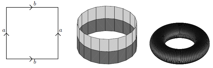
If the sides are identified with opposite orientation, the result is the Möbius strip:

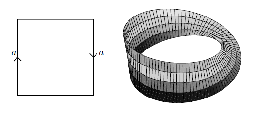
graphics grabbed from Lawson 03

Example

(stereographic projection)

For $n \in \mathbb{N}$ then there is a homeomorphism (def. ) between the n-sphere $S^n$ (example ) with one point $p \in S^n$ removed and the $n$-dimensional Euclidean space $\mathbb{R}^n$ (example ) with its metric topology (example ):

$$S^n \setminus \{p\} \overset{\phantom{AA}\simeq\phantom{AA}}{\longrightarrow} \mathbb{R}^n \,.$$

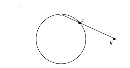
This homeomorphism is given by “stereographic projection”: One thinks of both the $n$-sphere as well as the Euclidean space $\mathbb{R}^n$ as topological subspaces (example ) of $\mathbb{R}^{n+1}$ in the standard way (example ), such that they intersect in the equator of the $n$-sphere. For $p \in S^n$ one of the corresponding poles, then the homeomorphism is the function which sends a point $x \in S^{n}\setminus \{p\}$ along the line connecting it with $p$ to the point $y$ where this line intersects the equatorial plane.

In the canonical ambient coordinates this stereographic projection is given as follows:

$$\array{ \mathbb{R}^{n+1} \supset \;\;\; & S^n \setminus (1,0, \cdots, 0) &\overset{\phantom{AA} \simeq \phantom{AA}}{\longrightarrow}& \mathbb{R}^{n} & \;\;\; \subset \mathbb{R}^{n+1} \\ & (x_1, x_2, \cdots, x_{n+1}) &\overset{\phantom{AAAA}}{\mapsto}& \frac{1}{1 - x_1} \left( 0 , x_2, \cdots, x_{n+1} \right) } \,.$$

Proof

First consider more generally the stereographic projection

$$\sigma \;\colon\; \mathbb{R}^{n+1} \backslash (1,0,\cdots, 0) \longrightarrow \mathbb{R}^n = \{x \in \mathbb{R}^{n.1} \,\vert\, x_1 = 0 \}$$

of the entire ambient space minus the point $p$ onto the equatorial plane, still given by mapping a point $x$ to the unique point $y$ on the equatorial hyperplane such that the points $p$, $x$ any $y$ sit on the same straight line.

This condition means that there exists $d \in \mathbb{R}$ such that

$$p + d(x-p) = y \,.$$

Since the only condition on $y$ is that $y_1 = 0$ this implies that

$$p_1 + d(x_1-p_1) = 0 \,.$$

This equation has a unique solution for $d$ given by

$$d = \frac{1}{1 - x_1}$$

and hence it follow that

$$\sigma(x_1, x_2, \cdots, x_{n+1}) = \frac{1}{1-x_1}(0,x_2, \cdots, x_n) \,$$

Since rational functions are continuous (example ), this function $\sigma$ is continuous and since the topology on $S^n\backslash p$ is the subspace topology under the canonical embedding $S^n \backslash p \subset \mathbb{R}^{n+1} \backslash p$ it follows that the restriction

$$\sigma\vert_{S^n \backslash p} \;\colon\; S^n\backslash p \longrightarrow \mathbb{R}^n$$

is itself a continuous function (because its pre-images are the restrictions of the pre-images of $\sigma$ to $S^n\backslash p$).

To see that $\sigma \vert_{S^n \backslash p}$ is a bijection of the underlying sets we need to show that for every

$$(0, y_2, \cdots, y_{n+1})$$

there is a unique $(x_1, \cdots , x_{n+1})$ satisfying

1. $(x_1, \cdots, x_{n+1}) \in S^{n} \backslash \{p\}$, hence

   1. $x_1 \lt 1$;

   2. $\underoverset{i = 1}{n+1}{\sum} (x_i)^2 = 1$;

2. $\underset{i \in \{2, \cdots, n+1\}}{\forall} \left(y_i = \frac{x_i}{1-x_1} \right)$.

The last condition uniquely fixes the $x_{i \geq 2}$ in terms of the given $y_{i \geq 2}$ and the remaining $x_1$, as

$$x_{i \geq 2} = y_i \cdot (1-x_1) \,.$$

With this, the second condition says that

$$(x_1)^2 + (1-x_1)^2 \underset{r^2}{\underbrace{\underoverset{i = 2}{n+1}{\sum}(y_i)^2}} = 1$$

hence equivalently that

$$(r^2 + 1) (x_1)^2 - (2 r^2) x_1 + (r^2 - 1) = 0 \,.$$

By the quadratic formula the solutions of this equation are

$$\begin{aligned} x_1 & = \frac { 2 r^2 \pm \sqrt{ 4 r^4 - 4 (r^4 - 1) } } { 2 (r^2 + 1) } \\ & = \frac { 2 r^2 \pm 2 } { 2 r^2 + 2 } \end{aligned} \,.$$

The solution $\frac{ 2 r^2 + 2 }{ 2 r^2 + 2 } = 1$ violates the first condition above, while the solution $\frac{ 2 r^2 - 2 }{ 2 r^2 + 2 } \lt 1$ satisfies it.

Therefore we have a unique solution, given by

$$\left( \sigma\vert_{S^n \backslash \{p\}} \right)^{-1}(0,y_2, \cdots, y_{n+1}) \;=\; \left( \frac{2 r^2 - 2}{2 r^2 +2} , \left( 1- \frac{2 r^2 - 2}{2 r^2 +2} \right) y_2 , \cdots , \left( 1- \frac{2 r^2 - 2}{2 r^2 +2} \right) y_{n+1} \right)$$

In particular therefore also an inverse function to the stereographic projection exists and is a rational function, hence continuous by example . So we have exhibited a homeomorphism as required.

$\,$

Important examples of pairs of spaces that are not homeomorphic include the following:

Theorem

(topological invariance of dimension)

For $n_1, n_2 \in \mathbb{N}$ but $n_1 \neq n_2$, then the Euclidean spaces $\mathbb{R}^{n_1}$ and $\mathbb{R}^{n_2}$ (example , example ) are not homeomorphic.

More generally, an open subset in $\mathbb{R}^{n_1}$ is never homeomorphic to an open subset in $\mathbb{R}^{n_2}$ if $n_1 \neq n_2$.

The proofs of theorem are not elementary, in contrast to how obvious the statement seems to be intuitively. One approach is to use tools from algebraic topology: One assigns topological invariants to topological spaces, notably classes in ordinary cohomology or in topological K-theory), quantities that are invariant under homeomorphism, and then shows that these classes coincide for $\mathbb{R}^{n_1} - \{0\}$ and for $\mathbb{R}^{n_2} - \{0\}$ precisely only if $n_1 = n_2$.

One indication that topological invariance of dimension is not an elementary consequence of the axioms of topological spaces is that a related “intuitively obvious” statement is in fact false: One might think that there is no surjective continuous function $\mathbb{R}^{n_1} \to \mathbb{R}^{n_2}$ if $n_1 \lt n_2$. But there are: these are called the Peano curves.

$\,$

Separation axioms

The plain definition of topological space (above) happens to admit examples where distinct points or distinct subsets of the underlying set appear as more-or-less unseparable as seen by the topology on that set.

The extreme class of examples of topological spaces in which the open subsets do not distinguish distinct underlying points, or in fact any distinct subsets, are the codiscrete spaces (example ). This does occur in practice:

Example

(real numbers quotiented by rational numbers)

Consider the real line $\mathbb{R}$ regarded as the 1-dimensional Euclidean space (example ) with its metric topology (example ) and consider the equivalence relation $\sim$ on $\mathbb{R}$ which identifies two real numbers if they differ by a rational number:

$$\left( x \sim y \right) \;\Leftrightarrow\; \left( \underset{p/q \in \mathbb{Q} \subset \mathbb{R}}{\exists} \left( x = y + p/q \right) \right) \,.$$

Then the quotient topological space (def. )

$$\mathbb{R}/\mathbb{Q} \;\coloneqq\; \mathbb{R}/\sim$$

is a codiscrete topological space (def. ), hence its topology does not distinguish any distinct proper subsets.

Here are some less extreme examples:

Example

(open neighbourhoods in the Sierpinski space)

Consider the Sierpinski space from example , whose underlying set consists of two points $\{0,1\}$, and whose open subsets form the set $\tau = \{ \emptyset, \{1\}, \{0,1\} \}$. This means that the only (open) neighbourhood of the point $\{0\}$ is the entire space. Incidentally, also the topological closure of $\{0\}$ (def. ) is the entire space.

Example

(line with two origins)

Consider the disjoint union space $\mathbb{R} \sqcup \mathbb{R}$ (example ) of two copies of the real line $\mathbb{R}$ regarded as the 1-dimensional Euclidean space (example ) with its metric topology (example ), which is equivalently the product topological space (example ) of $\mathbb{R}$ with the discrete topological space on the 2-element set (example ):

$$\mathbb{R} \sqcup \mathbb{R} \;\simeq\; \mathbb{R} \times Disc(\{0,1\})$$

Moreover, consider the equivalence relation on the underlying set which identifies every point $x_i$ in the $i$th copy of $\mathbb{R}$ with the corresponding point in the other, the $(1-i)$th copy, except when $x = 0$:

$$\left( x_i \sim y_j \right) \;\Leftrightarrow\; \left( \left( x = y \right) \,\text{and}\, \left( \left( x \neq 0 \right) \,\text{or}\, \left( i = j \right) \right) \right) \,.$$

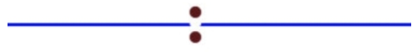
The quotient topological space by this equivalence relation (def. )

$$\left( \mathbb{R} \sqcup \mathbb{R} \right)/\sim$$

is called the line with two origins. These “two origins” are the points $0_0$ and $0_1$.

We claim that in this space every neighbourhood of $0_0$ intersects every neighbourhood of $0_1$.

Because, by definition of the quotient space topology, the open neighbourhoods of $0_i \in \left( \mathbb{R} \sqcup \mathbb{R} \right)/\sim$ are precisely those that contain subsets of the form

$$(-\epsilon, \epsilon)_i \;\coloneqq\; (-\epsilon,0) \cup \{0_i\} \cup (0,\epsilon) \,.$$

But this means that the “two origins” $0_0$ and $0_1$ may not be separated by neighbourhoods, since the intersection of $(-\epsilon, \epsilon)_0$ with $(-\epsilon, \epsilon)_i$ is always non-empty:

$$(-\epsilon, \epsilon)_0 \cap (-\epsilon, \epsilon)_1 \;=\; (-\epsilon, 0) \cup (0, \epsilon) \,.$$

In many applications one wants to exclude at least some such exotic examples of topological spaces from the discussion and instead concentrate on those examples for which the topology recognizes the separation of distinct points, or of more general disjoint subsets. The relevant conditions to be imposed on top of the plain axioms of a topological space are hence known as separation axioms which we discuss in the following.

These axioms are all of the form of saying that two subsets (of certain kinds) in the topological space are ‘separated’ from each other in one sense if they are ‘separated’ in a (generally) weaker sense. For example the weakest axiom (called $T_0$) demands that if two points are distinct as elements of the underlying set of points, then there exists at least one open subset that contains one but not the other.

In this fashion one may impose a hierarchy of stronger axioms. For example demanding that given two distinct points, then each of them is contained in some open subset not containing the other ($T_1$) or that such a pair of open subsets around two distinct points may in addition be chosen to be disjoint ($T_2$). Below in Tn-spaces we discuss the following hierarchy:

the main separation axioms

number	name	statement	reformulation
$T_0$	Kolmogorov	given two distinct points, at least one of them has an open neighbourhood not containing the other point	every irreducible closed subset is the closure of at most one point
$T_1$		given two distinct points, both have an open neighbourhood not containing the other point	all points are closed
$T_2$	Hausdorff	given two distinct points, they have disjoint open neighbourhoods	the diagonal is a closed map
$T_{\gt 2}$		$T_1$ and…	all points are closed and…
$T_3$	regular Hausdorff	…given a point and a closed subset not containing it, they have disjoint open neighbourhoods	…every neighbourhood of a point contains the closure of an open neighbourhood
$T_4$	normal Hausdorff	…given two disjoint closed subsets, they have disjoint open neighbourhoods	…every neighbourhood of a closed set also contains the closure of an open neighbourhood … every pair of disjoint closed subsets is separated by an Urysohn function

The condition, $T_2$, also called the Hausdorff condition is the most common among all separation axioms. Historically this axiom was originally taken as part of the definition of topological spaces, and it is still often (but by no means always) considered by default.

However, there are respectable areas of mathematics that involve topological spaces where the Hausdorff axiom fails, but a weaker axiom is still satisfied, called sobriety. This is the case notably in algebraic geometry (schemes are sober) and in computer science (Vickers 89). These sober topological spaces are singled out by the fact that they are entirely characterized by their sets of open subsets with their union and intersection structure (as in def. ) and may hence be understood independently from their underlying sets of points. This we discuss further below.

hierarchy of separation axioms
$\array{ &&&\text{metric space} \\ &&& \Downarrow \\ &&& \vdots \\ &&& \Downarrow \\ &&& T_4 = \text{normal Hausdorff} \\ &&& \Downarrow \\ &&& T_3 = \text{regular Hausdorff} \\ &&& \Downarrow \\ &&& T_2 = \text{Hausdorff} \\ && \swArrow && \seArrow \\ \, & T_1 && && \text{sober} & \, \\ && \seArrow && \swArrow \\ &&& T_0 = \text{Kolmogorov} \\ }$

All separation axioms are satisfied by metric spaces (example , example below), from whom the concept of topological space was originally abstracted above. Hence imposing some of them may also be understood as gauging just how far one allows topological spaces to generalize away from metric spaces

$T_n$ spaces

There are many variants of separation axioms. The classical ones are labeled $T_n$ (for German “Trennungsaxiom”) with $n \in \{0,1,2,3,4,5\}$ or higher. These we now introduce in def. and def. .

Definition

(the first three separation axioms)

Let $(X,\tau)$ be a topological space (def. ).

For $x \neq y \in X$ any two points in the underlying set of $X$ which are not equal as elements of this set, consider the following propositions:

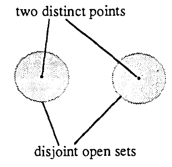
• (T0) There exists a neighbourhood of one of the two points which does not contain the other point.

• (T1) There exist neighbourhoods of both points which do not contain the other point.

• (T2) There exists neighbourhoods_ of both points which do not intersect each other.

graphics grabbed from Vickers 89

The topological space $X$ is called a $T_n$-topological space or just $T_n$-space, for short, if it satisfies condition $T_n$ above for all pairs of distinct points.

A $T_0$-topological space is also called a Kolmogorov space.

A $T_2$-topological space is also called a Hausdorff topological space.

For definiteness, we re-state these conditions formally. Write $x,y \in X$ for points in $X$, write $U_x, U_y \in \tau$ for open neighbourhoods of these points. Then:

• (T0) $\underset{x \neq y}{\forall} \left( \left( \underset{U_y}{\exists} \left( \{x\} \cap U_y = \emptyset \right) \right) \,\text{or}\, \left( \underset{U_x}{\exists} \left( U_x \cap \{y\} = \emptyset \right) \right) \right)$

• ((T1) $\underset{x \neq y}{\forall} \left(\underset{U_x,U_y}{\exists} \left(\left( \{x\} \cap U_y = \emptyset\right) \, \text{and} \, \left( U_x \cap \{y\} = \emptyset \right)\right) \right)$

• (T2) $\underset{x \neq y}{\forall} \left( \underset{U_x, U_y}{\exists} \left( U_x \cap U_y = \emptyset\right) \right)$

The following is evident but important:

Proposition

($T_n$ are topological properties of increasing strength)

The separation properties $T_n$ from def. are topological properties in that if two topological spaces are homeomorphic (def. ) then one of them satisfies $T_n$ precisely if the other does.

Moreover, these properties imply each other as

$$T2 \Rightarrow T1 \Rightarrow T0 \,.$$

Example

Examples of topological spaces that are not Hausdorff (def. ) include

1. the Sierpinski space (example ),

2. the line with two origins (example ),

3. the quotient topological space $\mathbb{R}/\mathbb{Q}$ (example ).

Example

(finite $T_1$-spaces are discrete)

For a finite topological space $(X,\tau)$, hence one for which the underlying set $X$ is a finite set, the following are equivalent:

1. $(X,\tau)$ is $T_1$ (def. );

2. $(X,\tau)$ is a discrete topological space (def. ).

Example

(metric spaces are Hausdorff)

Every metric space (def ), regarded as a topological space via its metric topology (example ) is a Hausdorff topological space (def. ).

Because for $x \neq y \in X$ two distinct points, then the distance $d(x,y)$ between them is positive number, by the non-degeneracy axiom in def. . Accordingly the open balls (def. )

$$B^\circ_x(d(x,y)) \supset \{x\} \phantom{AA} \text{and} \phantom{AA} B^\circ_y(d(x,y)) \supset \{y\}$$

are disjoint open neighbourhoods.

Example

(subspace of $T_n$-space is $T_n$)

Let $(X,\tau)$ be a topological space satisfying the $T_n$ separation axiom for some $n \in \{0,1,2\}$ according to def. . Then also every topological subspace $S \subset X$ (example ) satisfies $T_n$.

(Beware that this fails for some higher $n$ discussed below in def. . Open subspaces of normal spaces need not be normal.)

$\,$

Separation in terms of topological closures

The conditions $T_0$, $T_1$ and $T_2$ have the following equivalent formulation in terms of topological closures (def. ).

Proposition

($T_0$ in terms of topological closures)

A topological space $(X,\tau)$ is $T_0$ (def. ) precisely if the function $Cl(\{-\})$ that forms topological closures (def. ) of singleton subsets from the underlying set of $X$ to the set of irreducible closed subsets of $X$ (def. , which is well defined according to example ), is injective:

$$Cl(\{-\}) \;\colon\; X \overset{\phantom{AAA}}{\hookrightarrow} IrrClSub(X)$$

Proof

Assume first that $X$ is $T_0$. Then we need to show that if $x,y \in X$ are such that $Cl(\{x\}) = Cl(\{y\})$ then $x = y$. Hence assume that $Cl(\{x\}) = Cl(\{y\})$. Since the closure of a point is the complement of the union of the open subsets not containing the point (lemma ), this means that the union of open subsets that do not contain $x$ is the same as the union of open subsets that do not contain $y$:

$$\underset{ {U \subset X \, \text{open}} \atop { U \subset X\setminus \{x\} } }{\cup} \left( U \right) \;=\; \underset{ {U \subset X \, \text{open}} \atop { U \subset X\setminus \{y\} } }{\cup} \left( U \right)$$

But if the two points were distinct, $x \neq y$, then by $T_0$ one of the above unions would contain $x$ or $y$, while the other would not, in contradiction to the above equality. Hence we have a proof by contradiction.

Conversely, assume that $\left( Cl\{x\} = Cl\{y\}\right) \Rightarrow \left( x = y\right)$, and assume that $x \neq y$. Hence by contraposition $\mathrm{Cl}(\{x\}) \neq \mathrm{Cl}(\{y\})$. We need to show that there exists an open set which contains one of the two points, but not the other.

Assume there were no such open subset, hence that every open subset containing one of the two points would also contain then other. Then by lemma this would mean that $x \in \mathrm{Cl}(\{y\})$ and that $y \in \mathrm{Cl}(\{x\})$. But this would imply that $Cl(\{x\}) \subset \mathrm{Cl}(\{y\})$ and that $\mathrm{Cl}(\{y\}) \subset \mathrm{Cl}(\{x\})$, hence that $\mathrm{Cl}(\{x\}) = \mathrm{Cl}(\{y\})$. This is a proof by contradiction.

Proposition

($T_1$ in terms of topological closures)

A topological space $(X,\tau)$ is $T_1$ (def. ) precisely if all its points are closed points (def. ).

Proof

We have

$$\begin{aligned} \text{all points in}\, (X, \tau)\, \text{are closed} &\coloneqq\, \underset{x \in X}{\forall} \left( Cl(\{x\}) = \{x\} \right) \\ & \Leftrightarrow\, X \setminus \left( \underset{ { U \subset X\, \text{open} } \atop { x \notin U } }{\cup} \left( U \right) \right) \;=\; \{x\} \\ & \Leftrightarrow\, \left( \underset{ { U \subset X\, \text{open} } \atop { x \notin U } }{\cup} \left( U \right) \right) \;=\; X \setminus \{x\} \\ & \Leftrightarrow \underset{y \in Y}{\forall} \left( \left( \underset{ { U \subset X \, \text{open} } \atop { x \notin U } }{\exists} \left( y \in U \right) \right) \Leftrightarrow (y \neq x) \right) \\ & \Leftrightarrow\, (X,\tau)\, \text{is}\, T_1 \end{aligned} \,.$$

Here the first step is the reformulation of closure from lemma , the second is another application of the de Morgan law (prop. ), the third is the definition of union and complement, and the last one is manifestly by definition of $T_1$.

Proposition

($T_2$ in terms of topological closures)

A topological space $(X,\tau_X)$ is $T_2$=Hausdorff precisely if the image of the diagonal

$$\array{ X &\overset{\Delta_X}{\longrightarrow}& X \times X \\ x &\overset{\phantom{AAA}}{\mapsto}& (x,x) }$$

is a closed subset in the product topological space $(X \times X, \tau_{X \times X})$.

Proof

Observe that the Hausdorff condition is equivalently rephrased in terms of the product topology as: Every point $(x,y) \in X$ which is not on the diagonal has an open neighbourhood $U_{(x,y)} \times U_{(x,y)}$ which still does not intersect the diagonal, hence:

$$\begin{aligned} & (X,\tau)\,\text{Hausdorff} \\ \Leftrightarrow & \underset{(x,y) \in (X \times X) \setminus \Delta_X(X) }{\forall} \left( \underset{ { U_{(x,y)} \times V_{(x,y)} \in \tau_{X \times Y} } \atop { (x,y) \in U_{(x,y)} \times V_{(x,y)} } }{\exists} \left( U_{(x,y)} \times V_{(x,y)} \cap \Delta_X(X) = \emptyset \right) \right) \end{aligned}$$

Therefore if $X$ is Hausdorff, then the diagonal $\Delta_X(X) \subset X \times X$ is the complement of a union of such open sets, and hence is closed:

$$(X, \tau)\, \text{Hausdorff} \;\;\;\Rightarrow \;\;\; \Delta_X(X) = X \setminus \left( \underset{(x,y) \in (X \times X) \setminus \Delta_X(X)}{\cup} U_{(x,y)} \times V_{(x,y)} \right) \,.$$

Conversely, if the diagonal is closed, then (by lemma ) every point $(x,y) \in X \times X$ not on the diagonal, hence with $x \neq y$, has an open neighbourhood $U_{(x,y)} \times V_{(x,y)}$ still not intersecting the diagonal, hence so that $U_{(x,y)} \cap V_{(x,y)} = \emptyset$. Thus $(X,\tau)$ is Hausdorff.

$\,$

Further separation axioms

Clearly one may and does consider further variants of the separation axioms $T_0$, $T_1$ and $T_2$ from def. . Here we discuss two more:

Definition

Let $(X,\tau)$ be topological space (def. ).

Consider the following conditions

• (T3) The space $(X,\tau)$ is $T_1$ (def. ) and for $x \in X$ a point and $C \subset X$ a closed subset (def. ) not containing $x$, then there exist disjoint open neighbourhoods $U_x \supset \{x\}$ and $U_C \supset C$.

• (T4) The space $(X,\tau)$ is $T_1$ (def. ) and for $C_1, C_2 \subset X$ two disjoint closed subsets (def. ) then there exist disjoint open neighbourhoods $U_{C_i} \supset C_i$.

If $(X,\tau)$ satisfies $T_3$ it is said to be a $T_3$-space also called a regular Hausdorff topological space.

If $(X,\tau)$ satisfies $T_4$ it is to be a $T_4$-space also called a normal Hausdorff topological space.

Example

(metric spaces are normal Hausdorff)

Let $(X,d)$ be a metric space (def. ) regarded as a topological space via its metric topology (example ). Then this is a normal Hausdorff space (def. ).

Proof

By example metric spaces are $T_2$, hence in particular $T_1$. What we need to show is that given two disjoint closed subsets $C_1, C_2 \subset X$ then their exists disjoint open neighbourhoods $U_{C_1} \subset C_1$ and $U_{C_2} \supset C_2$.

Recall the function

$$d(S,-) \colon X \to \mathbb{R}$$

computing distances from a subset $S \subset X$ (example ). Then the unions of open balls (def. )

$$U_{C_1} \coloneqq \underset{x_1 \in C_1}{\cup} B^\circ_{x_1}( d(C_2,x_1)/2 )$$

and

$$U_{C_2} \coloneqq \underset{x_2 \in C_2}{\cup} B^\circ_{x_2}( d(C_1,x_2)/2 ) \,.$$

have the required properties.

Observe that:

Proposition

($T_n$ are topological properties of increasing strength)

The separation axioms from def. , def. are topological properties (def. ) which imply each other as

$$T_4 \Rightarrow T_3 \Rightarrow T_2 \Rightarrow T_1 \Rightarrow T_0 \,.$$

Proof

The implications

$$T_2 \Rightarrow T_1 \Rightarrow T_0$$

and

$$T_4 \Rightarrow T_3$$

are immediate from the definitions. The remaining implication $T_3 \Rightarrow T_2$ follows with prop. : This says that by assumption of $T_1$ then all points in $(X,\tau)$ are closed, and with this the condition $T_2$ is manifestly a special case of the condition for $T_3$.

Hence instead of saying “$X$ is $T_1$ and …” one could just as well phrase the conditions $T_3$ and $T_4$ as “$X$ is $T_2$ and …”, which would render the proof of prop. even more trivial.

The following shows that not every $T_2$-space/Hausdorff space is $T_3$/regular

Example

(K-topology)

Write

$$K \coloneqq \{1/n \,\vert\, n \in \mathbb{N}_{\geq 1}\} \subset \mathbb{R}$$

for the subset of natural fractions inside the real numbers.

Define a topological basis $\beta \subset P(\mathbb{R})$ on $\mathbb{R}$ consisting of all the open intervals as well as the complements of $K$ inside them:

$$\beta \;\coloneqq\; \left\{ (a,b), \,\vert\, a\lt b \in \mathbb{R} \right\} \,\cup\, \left\{ (a,b) \setminus K, \,\vert\, a\lt b \in \mathbb{R} \right\} \,.$$

The topology $\tau_{\beta} \subset P(\mathbb{R})$ which is generated from this topological basis is called the K-topology.

We may denote the resulting topological space by

$$\mathbb{R}_K \;\coloneqq\; ( \mathbb{R}, \tau_{\beta}\} \,.$$

This is a Hausdorff topological space (def. ) which is not a regular Hausdorff space, hence (by prop. ) in particular not a normal Hausdorff space (def. ).

$\,$

Further separation axioms in terms of topological closures

As before we have equivalent reformulations of the further separation axioms.

Proposition

($T_3$ in terms of topological closures)

A topological space $(X,\tau)$ is a regular Hausdorff space (def. ), precisely if all points are closed and for all points $x \in X$ with open neighbourhood $U \supset \{x\}$ there exists a smaller open neighbourhood $V \supset \{x\}$ whose topological closure $Cl(V)$ is still contained in $U$:

$$\{x\} \subset V \subset Cl(V) \subset U \,.$$

The proof of prop. is the direct specialization of the following proof for prop. to the case that $C = \{x\}$ (using that by $T_1$, which is part of the definition of $T_3$, the singleton subset is indeed closed, by prop. ).

Proposition

($T_4$ in terms of topological closures)

A topological space $(X,\tau)$ is normal Hausdorff space (def. ), precisely if all points are closed and for all closed subsets $C \subset X$ with open neighbourhood $U \supset C$ there exists a smaller open neighbourhood $V \supset C$ whose topological closure $Cl(V)$ is still contained in $U$:

$$C \subset V \subset Cl(V) \subset U \,.$$

Proof

In one direction, assume that $(X,\tau)$ is normal, and consider

$$C \subset U \,.$$

It follows that the complement of the open subset $U$ is closed and disjoint from $C$:

$$C \cap X \setminus U = \emptyset \,.$$

Therefore by assumption of normality of $(X,\tau)$, there exist open neighbourhoods with

$$V \supset C \,, \phantom{AA} W \supset X \setminus U \phantom{AA} \text{with} \phantom{AA} V \cap W = \emptyset \,.$$

But this means that

$$V \subset X \setminus W$$

and since the complement $X \setminus W$ of the open set $W$ is closed, it still contains the closure of $V$, so that we have

$$C \subset V \subset Cl(V) \subset X \setminus W \subset U$$

as required.

In the other direction, assume that for every open neighbourhood $U \supset C$ of a closed subset $C$ there exists a smaller open neighbourhood $V$ with

$$C \subset V \subset Cl(V) \subset U \,.$$

Consider disjoint closed subsets

$$C_1, C_2 \subset X \,, \phantom{AAA} C_1 \cap C_2 = \emptyset \,.$$

We need to produce disjoint open neighbourhoods for them.

From their disjointness it follows that

$$X \setminus C_2 \supset C_1$$

is an open neighbourhood. Hence by assumption there is an open neighbourhood $V$ with

$$C_1 \subset V \subset Cl(V) \subset X \setminus C_2 \,.$$

Thus

$$V \supset C_1 \,, \phantom{AAAA} X \setminus Cl(V) \supset C_2$$

are two disjoint open neighbourhoods, as required.

But the $T_4$/normality axiom has yet another equivalent reformulation, which is of a different nature, and will be important when we discuss paracompact topological spaces below:

The following concept of Urysohn functions is another approach of thinking about separation of subsets in a topological space, not in terms of their neighbourhoods, but in terms of continuous real-valued “indicator functions” that take different values on the subsets. This perspective will be useful when we consider paracompact topological spaces below.

But the Urysohn lemma (prop. below) implies that this concept of separation is in fact equivalent to that of normality of Hausdorff spaces.

Definition

(Urysohn function)

Let $(X,\tau)$ be a topological space, and let $A,B \subset X$ be disjoint closed subsets. Then an Urysohn function separating $A$ from $B$ is

• a continuous function $f \colon X \to [0,1]$

to the closed interval equipped with its Euclidean metric topology (example , example ), such that

• it takes the value 0 on $A$ and the value 1 on $B$:

  $$f(A) = \{0\} \phantom{AAA} \text{and} \phantom{AAA} f(B) = \{1\} \,.$$

Proposition

(Urysohn's lemma)

Let $X$ be a normal Hausdorff topological space (def. ), and let $A,B \subset X$ be two disjoint closed subsets of $X$. Then there exists an Urysohn function separating $A$ from $B$ (def. ).

Remark

Beware, the Urysohn function in prop. may take the values 0 or 1 even outside of the two subsets. The condition that the function takes value 0 or 1, respectively, precisely on the two subsets corresponds to “perfectly normal spaces”.

Proof

of Urysohn's lemma, prop.

Set

$$C_0 \coloneqq A \phantom{AAA} U_1 \coloneqq X \setminus B \,.$$

Since by assumption

$$A \cap B = \emptyset \,.$$

we have

$$C_0 \subset U_1 \,.$$

That $(X,\tau)$ is normal implies, by lemma , that every open neighbourhood $U \supset C$ of a closed subset $C$ contains a smaller neighbourhood $V$ together with its topological closure $Cl(V)$

$$U \subset V \subset Cl(V) \subset C \,.$$

Apply this fact successively to the above situation to obtain the following infinite sequence of nested open subsets $U_r$ and closed subsets $C_r$

$$\array{ C_0 && && && &\subset& && && && U_1 \\ C_0 && &\subset& && U_{1/2} &\subset& C_{1/2} && &\subset& && U_1 \\ C_0 &\subset& U_{1/4} &\subset& C_{1/4} &\subset& U_{1/2} &\subset& C_{1/2} &\subset& U_{3/4} &\subset& C_{3/4} &\subset& U_1 }$$

and so on, labeled by the dyadic rational numbers $\mathbb{Q}_{dy} \subset \mathbb{Q}$ within $(0,1]$

$$\{ U_{r} \subset X \}_{r \in (0,1] \cap \mathbb{Q}_{dy}}$$

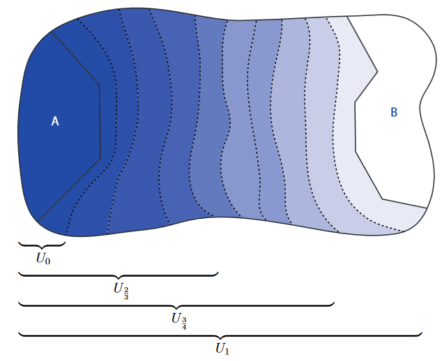
with the property

$$\underset{r_1 \lt r_2 \, \in (0,1] \cap \mathbb{Q}_{dy}}{\forall} \left( U_{r_1} \subset Cl(U_{r_1}) \subset U_{r_2} \right) \,.$$

Define then the function

$$f \;\colon\; X \longrightarrow [0,1]$$

to assign to a point $x \in X$ the infimum of the labels of those open subsets in this sequence that contain $x$:

$$f(x) \coloneqq \underset{U_r \supset \{x\}}{\lim} r$$

Here the limit is over the directed set of those $U_r$ that contain $x$, ordered by reverse inclusion.

This function clearly has the property that $f(A) = \{0\}$ and $f(B) = \{1\}$. It only remains to see that it is continuous.

To this end, first observe that

$$\array{ (\star) && \left( x \in Cl(U_r) \right) &\Rightarrow& \left( f(x) \leq r \right) \\ (\star\star) && \left( x \in U_r \right) &\Leftarrow& \left( f(x) \lt r \right) } \,.$$

Here it is immediate from the definition that $(x \in U_r) \Rightarrow (f(x) \leq r)$ and that $(f(x) \lt r) \Rightarrow (x \in U_r \subset Cl(U_r))$. For the remaining implication, it is sufficient to observe that

$$(x \in \partial U_r) \Rightarrow (f(x) = r) \,,$$

where $\partial U_r \coloneqq Cl(U_r) \setminus U_r$ is the boundary of $U_r$.

This holds because the dyadic numbers are dense in $\mathbb{R}$. (And this would fail if we stopped the above decomposition into $U_{a/2^n}$-s at some finite $n$.) Namely, in one direction, if $x \in \partial U_r$ then for every small positive real number $\epsilon$ there exists a dyadic rational number $r'$ with $r \lt r' \lt r + \epsilon$, and by construction $U_{r'} \supset Cl(U_r)$ hence $x \in U_{r'}$. This implies that $\underset{U_r \supset \{x\}}{\lim} = r$.

Now we claim that for all $\alpha \in [0,1]$ then

1. $f^{-1}(\,(\alpha, 1]\,) = \underset{r \gt \alpha}{\cup} \left( X \setminus Cl(U_r) \right)$

2. $f^{-1}(\,[0,\alpha)\,) = \underset{r \lt \alpha}{\cup} U_r$

Thereby $f^{-1}(\,(\alpha, 1]\,)$ and $f^{-1}(\,[0,\alpha)\,)$ are exhibited as unions of open subsets, and hence they are open.

Regarding the first point:

$$\begin{aligned} & x \in f^{-1}( \,(\alpha,1]\, ) \\ \Leftrightarrow\, & f(x) \gt \alpha \\ \Leftrightarrow\, & \underset{r \gt \alpha}{\exists} (f(x) \gt r) \\ \overset{(\star)}{\Rightarrow}\, & \underset{r \gt \alpha}{\exists} \left( x \notin Cl(U_r) \right) \\ \Leftrightarrow\, & x \in \underset{r \gt \alpha}{\cup} \left(X \setminus Cl(U_r)\right) \end{aligned}$$

and

$$\begin{aligned} & x \in \underset{r \gt \alpha}{\cup} \left(X \setminus Cl(U_r)\right) \\ \Leftrightarrow\, & \underset{r \gt \alpha}{\exists} \left( x \notin Cl(U_r) \right) \\ \Rightarrow\, & \underset{r \gt \alpha}{\exists} \left( x \notin U_r \right) \\ \overset{(\star \star)}{\Rightarrow}\, & \underset{r \gt \alpha}{\exists} \left( f(x) \geq r \right) \\ \Leftrightarrow\, & f(x) \gt \alpha \\ \Leftrightarrow\, & x \in f^{-1}(\, (\alpha,1] \,) \end{aligned} \,.$$

Regarding the second point:

$$\begin{aligned} & x \in f^{-1}(\, [0,\alpha) \,) \\ \Leftrightarrow\, & f(x) \lt \alpha \\ \Leftrightarrow\, & \underset{r \lt \alpha}{\exists}( f(x) \lt r ) \\ \overset{(\star \star)}{\Rightarrow}\, & \underset{r \lt \alpha}{\exists }( x \in U_r ) \\ \Leftrightarrow\, & x \in \underset{r \lt \alpha}{\cup} U_r \end{aligned}$$

and

$$\begin{aligned} & x \in \underset{r \lt \alpha}{\cup} U_r \\ \Leftrightarrow\, & \underset{r \lt \alpha}{\exists }( x \in U_r ) \\ \overset{}{\Rightarrow}\, & \underset{r \lt \alpha}{\exists }( x \in Cl(U_r) ) \\ \overset{(\star)}{\Rightarrow}\, & \underset{r \lt \alpha}{\exists }( f(x) \leq r ) \\ \Leftrightarrow\, & f(x) \lt \alpha \\ \Leftrightarrow\, & x \in f^{-1}(\, [0,\alpha) \,) \end{aligned} \,.$$

(In these derivations we repeatedly use that $(0,1] \cap \mathbb{Q}_{dy}$ is dense in $[0,1]$ (def. ), and we use the contrapositions of $(\star)$ and $(\star \star)$.)

Now since the subsets $\{ [0,\alpha), (\alpha,1]\}_{\alpha \in [0,1]}$ form a sub-base (def. ) for the Euclidean metric topology on $[0,1]$, it follows that all pre-images of $f$ are open, hence that $f$ is continuous.

As a corollary of Urysohn's lemma we obtain yet another equivalent reformulation of the normality of topological spaces, this one now of a rather different character than the re-formulations in terms of explicit topological closures considered above:

Proposition

(normality equivalent to existence of Urysohn functions)

A $T_1$-space (def. ) is normal (def. ) precisely if it admits Urysohn functions (def ) separating every pair of disjoint closed subsets.

Proof

In one direction this is the statement of the Urysohn lemma, prop. .

In the other direction, assume the existence of Urysohn functions (def. ) separating all disjoint closed subsets. Let $A, B \subset X$ be disjoint closed subsets, then we need to show that these have disjoint open neighbourhoods.

But let $f \colon X \to [0,1]$ be an Urysohn function with $f(A) = \{0\}$ and $f(B) = \{1\}$ then the pre-images

$$U_A \coloneqq f^{-1}([0,1/3) \phantom{AAA} U_B \coloneqq f^{-1}((2/3,1])$$

are disjoint open neighbourhoods as required.

$\,$

$T_n$ reflection

While the topological subspace construction preserves the $T_n$-property for $n \in \{0,1,2\}$ (example ) the construction of quotient topological spaces in general does not, as shown by examples and .

Further below we will see that, generally, among all universal constructions in the category Top of all topological spaces those that are limits preserve the $T_n$ property, while those that are colimits in general do not.

But at least for $T_0$, $T_1$ and $T_2$ there is a universal way, called reflection (prop. below), to approximate any topological space “from the left” by a $T_n$ topological spaces

Hence if one wishes to work within the full subcategory of the $T_n$-spaces among all topological space, then the correct way to construct quotients and other colimits (see below) is to first construct them as usual quotient topological spaces (example ), and then apply the $T_n$-reflection to the result.

Proposition

($T_n$-reflection)

Let $n \in \{0,1,2\}$. Then for every topological space $X$ there exists

1. a $T_n$-topological space $T_n X$

2. a continuous function

   $$t_n(X) \;\colon\; X \longrightarrow T_n X$$

   called the $T_n$-reflection of $X$,

which is the “closest approximation from the left” to $X$ by a $T_n$-topological space, in that for $Y$ any $T_n$-space, then continuous functions of the form

$$f \;\colon\; X \longrightarrow Y$$

are in bijection with continuous function of the form

$$\tilde f \;\colon\; T_n X \longrightarrow Y$$

and such that the bijection is constituted by

$$f = \tilde f \circ t_n(X) \;\colon\; X \overset{ t_n(X)}{\longrightarrow} T_n X \overset{\tilde f}{\longrightarrow} Y \phantom{AAAA}i.e.: \phantom{AAA} \array{ X && \overset{f}{\longrightarrow} && Y \\ & {}_{\mathllap{t_n(X)}}\searrow && \nearrow_{\mathrlap{\tilde f}} \\ && T_n X } \,.$$

• For $n = 0$ this is known as the Kolmogorov quotient construction (see prop. below).

• For $n = 2$ this is known as Hausdorff reflection or Hausdorffication or similar.

Moreover, the operation $T_n(-)$ extends to continuous functions $f \colon X \to Y$

$$(X \overset{f}{\to} Y) \;\mapsto\; (T_n X \overset{T_n f}{\to} T_n Y)$$

such as to preserve composition of functions as well as identity functions:

$$T_n g \circ T_n f = T_n(g \circ f) \phantom{AA} \,, \phantom{AA} T_n id_X = id_{T_n X} \,$$

Finally, the comparison map is compatible with this in that

$$t_n(Y) \circ f = T_n(f) \circ t_n(X) \phantom{AAAA} i.e.: \phantom{AAAA} \array{ X &\overset{f}{\longrightarrow}& Y \\ {}^{\mathllap{t_n(X)}}\downarrow && \downarrow^{\mathrlap{t_n(Y)}} \\ T_n X &\underset{T_n(f)}{\longrightarrow}& T_n Y } \,.$$

We prove this via a concrete construction of $T_n$-reflection in prop. below. But first we pause to comment on the bigger picture of the $T_n$-reflection:

Remark

(reflective subcategories)

In the language of category theory (remark ) the $T_n$-reflection of prop. says that

1. $T_n(-)$ is a functor $T_n \;\colon\; Top \longrightarrow Top_{T_n}$ from the category Top of topological spaces to the full subcategory $Top_{T_n} \overset{\iota}{\hookrightarrow} Top$ of Hausdorff topological spaces;

2. $t_n(X) \colon X \to T_n X$ is a natural transformation from the identity functor on Top to the functor $\iota \circ T_n$

3. $T_n$-topological spaces form a reflective subcategory of all topological spaces in that $T_n$ is left adjoint to the inclusion functor $\iota$; this situation is denoted as follows:

   $$Top_{T_n} \underoverset{\underset{\phantom{A}\iota\phantom{A}}{\hookrightarrow}}{\overset{\phantom{A}H\phantom{A}}{\longleftarrow}}{\bot} Top \,.$$

Generally, an adjunction between two functors

$$L \;\colon\; \mathcal{C} \leftrightarrow \mathcal{D} \;\colon\; R$$

is for all pairs of objects $c \in \mathcal{C}$, $d \in \mathcal{D}$ a bijection between sets of morphisms of the form

$$\left\{ L(c) \longrightarrow d \right\} \phantom{A} \leftrightarrow \phantom{A} \left\{ c \longrightarrow R(d) \right\} \,.$$

i.e.

$$Hom_{\mathcal{D}}(L(c), d) \underoverset{\phantom{AA}\simeq \phantom{AA}}{\phi_{c,d}}{\longrightarrow} Hom_{\mathcal{C}}(c, R(d))$$

and such that these bijections are “natural” in that they for all pairs of morphisms $f \colon c' \to c$ and $g \colon d \to d'$ then the folowing diagram commutes:

$$\array{ Hom_{\mathcal{D}}(L(c), d) &\underoverset{\phantom{AA}\simeq\phantom{AA}}{\phi_{c,d}}{\longrightarrow}& Hom_{\mathcal{C}}(c, R(d)) \\ {\mathllap{g \circ (-) \circ L(f)}}\downarrow && \downarrow{\mathrlap{ R(g) \circ (-) \circ f }} \\ Hom_{\mathcal{C}}(L(c'), d') &\underoverset{\phantom{AA}\simeq\phantom{AA}}{\phi_{c',d'}}{\longrightarrow}& Hom_{\mathcal{D}}(c', R(d')) } \,.$$

One calls the image under $\phi_{c,L(c)}$ of the identity morphism $id_{L(x)}$ the unit of the adjunction, written

$$\eta_x \;\colon\; c \longrightarrow R(L(c)) \,.$$

One may show that it follows that the image $\tilde f$ under $\phi_{c,d}$ of a general morphism $f \colon c \to d$ (called the adjunct of $f$) is given by this composite:

$$\tilde f \;\colon\; c \overset{\eta_c}{\longrightarrow} R(L(c)) \overset{R(f)}{\longrightarrow} R(d) \,.$$

In the case of the reflective subcategory inclusion $(T_n \dashv \iota)$ of the category of $T_n$-spaces into the category Top of all topological spaces this adjunction unit is precisely the $T_n$-reflection $t_n(X) \colon X \to \iota( T_n(X))$ (only that we originally left the re-embedding $\iota$ notationally implicit).

$\,$

There are various ways to see the existence and to construct the $T_n$-reflections. The following is the quickest way to see the existence, even though it leaves the actual construction rather implicit.

Proposition

($T_n$-reflection via explicit quotients)

Let $n \in \{0,1,2\}$. Let $(X,\tau)$ be a topological space and consider the equivalence relation $\sim$ on the underlying set $X$ for which $x_1 \sim x_2$ precisely if for every surjective continuous function $f \colon X \to Y$ into any $T_n$-topological space $Y$ (def. ) we have $f(x_1) = f(x_2)$:

$$(x_1 \sim x_2) \;\coloneqq\; \underset{ { Y \in Top_{T_n} } \atop { X \underoverset{\text{surjective}}{f}{\to} Y } }{\forall} \left( f(x) = f(y) \right) \,.$$

Then

1. the set of equivalence classes

   $$T_n X \coloneqq X /{\sim}$$

   equipped with the quotient topology (example ) is a $T_n$-topological space,

2. the quotient projection

   $$\array{ X & \overset{t_n(X)}{\longrightarrow} & X/{\sim} \\ x &\overset{\phantom{AAA}}{\mapsto}& [x] }$$

   exhibits the $T_n$-reflection of $X$, according to prop. .

Proof

First we observe that every continuous function $f \colon X \longrightarrow Y$ into a $T_n$-topological space $Y$ factors uniquely, via $t_n(X)$ through a continuous function $\tilde f$ (this makes use of the “universal property” of the quotient topology, which we dwell on a bit more below in example ):

$$f = \tilde f \circ t_n(X)$$

Clearly this continuous function $\tilde f$ is unique if it exists, because its underlying function of sets must be given by

$$\tilde f \colon [x] \mapsto f(x) \,.$$

First observe that this is indeed well defined as a function of underlying sets. To that end, factor $f$ through its image $f(X)$

$$f \;\colon\; X \longrightarrow f(X) \hookrightarrow Y$$

equipped with its subspace topology as a subspace of $Y$ (example ). By prop. also the image $f(X)$ is a $T_n$-topological space, since $Y$ is. This means that if two elements $x_1, x_2 \in X$ have the same equivalence class, then, by definition of the equivalence relation, they have the same image under all continuous surjective functions into a $T_n$-space, hence in particular they have the same image under $f \colon X \overset{\text{surjective}}{\longrightarrow} f(X) \hookrightarrow Y$:

$$\begin{aligned} ( [x_1] = [x_2]) & \Leftrightarrow\, (x_1 \sim x_2) \\ & \Rightarrow\, ( f(x_1) = f(x_2) ) \,. \end{aligned}$$

This shows that $\tilde f$ is well defined as a function between sets.

To see that $\tilde f$ is also continuous, consider $U \in Y$ an open subset. We need to show that the pre-image $\tilde f^{-1}(U)$ is open in $X/\sim$. But by definition of the quotient topology (example ), this is open precisely if its pre-image under the quotient projection $t_n(X)$ is open, hence precisely if

$$\begin{aligned} (t_n(X))^{-1} \left( \tilde f^{-1}\left(U\right) \right) & = \left( \tilde f \circ t_n(X) \right)^{-1}(U) \\ & = f^{-1}(U) \end{aligned}$$

is open in $X$. But this is the case by the assumption that $f$ is continuous. Hence $\tilde f$ is indeed the unique continuous function as required.

What remains to be seen is that $T_n X$ as constructed is indeed a $T_n$-topological space. Hence assume that $[x] \neq [y] \in T_n X$ are two distinct points. Depending on the value of $n$, need to produce open neighbourhoods around one or both of these points not containing the other point and possibly disjoint to each other.

Now by definition of $T_n X$ the assumption $[x] \neq [y]$ means that there exists a $T_n$-topological space $Y$ and a surjective continuous function $f \colon X \overset{surjective}{\longrightarrow} Y$ such that $f(x) \neq f(y) \in Y$:

$$( [x_1] \neq [x_2] ) \;\Leftrightarrow\; \underset{ { Y \in Top_{T_m} \atop { X \underoverset{\text{surjective}}{f}{\longrightarrow} Y } } }{\exists} \left( f(x_1) \neq f(x_2) \right) \,.$$

Accordingly, since $Y$ is $T_n$, there exist the respective kinds of neighbourhoods around $f(x_1)$ and $f(x_2)$ in $Y$. Moreover, by the previous statement there exists the continuous function $\tilde f \colon T_n X \to Y$ with $\tilde f([x_1]) = f(x_1)$ and $\tilde f([x_2]) = f(x_2)$. By the nature of continuous functions, the pre-images of these open neighbourhoods in $Y$ are still open in $X$ and still satisfy the required disjunction properties. Therefore $T_n X$ is a $T_n$-space.

Here are alternative constructions of the reflections:

Proposition

(Kolmogorov quotient)

Let $(X,\tau)$ be a topological space. Consider the relation on the underlying set by which $x_1 \sim x_2$ precisely if neither $x_i$ has an open neighbourhood not containing the other. This is an equivalence relation. The quotient topological space $X \to X/\sim$ by this equivalence relation (def. ) exhibits the $T_0$-reflection of $X$ according to prop. .

A more explicit construction of the Hausdorff quotient than given by prop. is rather more involved. The issue is that the relation “$x$ and $y$ are not separated by disjoint open neighbourhoods” is not transitive;

Proposition

(more explicit Hausdorff reflection)

For $(Y,\tau_Y)$ a topological space, write $r_Y \subset Y \times Y$ for the transitive closure of the relation given by the topological closure $Cl(\Delta_Y)$ of the image of the diagonal $\Delta_Y \colon Y \hookrightarrow Y \times Y$.

$$r_Y \coloneqq Trans(Cl(Delta_Y)) \,.$$

Now for $(X,\tau_X)$ a topological space, define by induction for each ordinal number $\alpha$ an equivalence relation $r^\alpha$ on $X$ as follows, where we write $q^\alpha \colon X \to H^\alpha(X)$ for the corresponding quotient topological space projection:

We start the induction with the trivial equivalence relation:

• $r^0_X \coloneqq \Delta_X$;

For a successor ordinal we set

• $r_X^{\alpha+1} \coloneqq \left\{ (a,b) \in X \times X \,\vert\, (q^\alpha(a), q^\alpha(b)) \in r_{H^\alpha(X)} \right\}$

and for a limit ordinal $\alpha$ we set

• $r_X^\alpha \coloneqq \underset{\beta \lt \alpha}{\cup} r_X^\beta$.

Then:

1. there exists an ordinal $\alpha$ such that $r_X^\alpha = r_X^{\alpha+1}$

2. for this $\alpha$ then $H^\alpha(X) = H(X)$ is the Hausdorff reflection from prop. .

A detailed proof is spelled out in (vanMunster 14, section 4).

Example

(Hausdorff reflection of the line with two origins)

The Hausdorff reflection ($T_2$-reflection, prop. )

$$T_2 \;\colon\; Top \longrightarrow Top_{Haus}$$

of the line with two origins from example is the real line itself:

$$T_2\left( \left( \mathbb{R} \sqcup \mathbb{R} \right)/\sim \right) \;\simeq\; \mathbb{R} \,.$$

$\,$

Sober spaces

While the original formulation of the separation axioms $T_n$ from def. and def. clearly does follow some kind of pattern, its equivalent reformulation in terms of closure conditions in prop. , prop. , prop , prop. and prop. suggests rather different patterns. Therefore it is worthwhile to also consider separation-like axioms that are not among the original list.

In particular, the alternative characterization of the $T_0$-condition in prop. immediately suggests the following strengthening, different from the $T_1$-condition (see example below):

Definition

(sober topological space)

A topological space $(X,\tau)$ is called a sober topological space precisely if every irreducible closed subspace (def. ) is the topological closure (def. ) of a unique point, hence precisely if the function

$$Cl(\{-\}) \;\colon\; X \longrightarrow IrrClSub(X)$$

from the underlying set of $X$ to the set of irreducible closed subsets of $X$ (def. , well defined according to example ) is bijective.

Proposition

(sober implies $T_0$)

Every sober topological space (def. ) is $T_0$ (def. ).

Proof

By prop. .

Proposition

(Hausdorff spaces are sober)

Every Hausdorff topological space (def. ) is a sober topological space (def. ).

More specifically, in a Hausdorff topological space the irreducible closed subspaces (def. ) are precisely the singleton subspaces (def. ).

Hence, by example , in particular every metric space with its metric topology (example ) is sober.

Proof

The second statement clearly implies the first. To see the second statement, suppose that $F$ is an irreducible closed subspace which contained two distinct points $x \neq y$. Then by the Hausdorff property there would be disjoint neighbourhoods $U_x, U_y$, and hence it would follow that the relative complements $F \setminus U_x$ and $F \setminus U_y$ were distinct closed proper subsets of $F$ with

$$F = (F \setminus U_x) \cup (F \setminus U_y)$$

in contradiction to the assumption that $F$ is irreducible.

This proves by contradiction that every irreducible closed subset is a singleton. Conversely, generally the topological closure of every singleton is irreducible closed, by example .

By prop. and prop. we have the implications on the right of the following diagram:

separation axioms
$\array{\\ &&& T_2 = \text{Hausdorff} \\ && \swArrow && \seArrow \\ \, & T_1 && && \text{sober} & \, \\ && \seArrow && \swArrow \\ &&& T_0 = \text{Kolmogorov} \\ }$

But there there is no implication betwee $T_1$ and sobriety:

Proposition

The intersection of the classes of sober topological spaces (def. ) and $T_1$-topological spaces (def. ) is not empty, but neither class is contained within the other.

That the intersection is not empty follows from prop. . That neither class is contained in the other is shown by the following counter-examples:

Example

($T_1$ neither implies nor is implied by sobriety)

• The Sierpinski space (def. ) is sober, but not $T_1$.

• The cofinite topology (example ) on a non-finite set is $T_1$ but not sober.

Finally, sobriety is indeed strictly weaker that Hausdorffness:

Example

(schemes are sober but in general not Hausdorff)

The Zariski topology on an affine space (example ) or more generally on the prime spectrum of a commutative ring (example ) is

1. sober (def );

2. in general not Hausdorff (def. ).

For details see at Zariski topology this prop and this example.

Frames of opens

What makes the concept of sober topological spaces special is that for them the concept of continuous functions may be expressed entirely in terms of the relations between their open subsets, disregarding the underlying set of points of which these opens are in fact subsets.

Recall from example that for every continuous function $f \colon (X, \tau_X) \to (Y, \tau_Y)$ the pre-image function $f^{-1} \colon \tau_Y \to \tau_X$ is a frame homomorphism (def. ).

For sober topological spaces the converse holds:

Proposition

If $(X,\tau_X)$ and $(Y,\tau_Y)$ are sober topological spaces (def. ), then for every frame homomorphism (def. )

$$\tau_X \longleftarrow \tau_Y \;\colon\; \phi$$

there is a unique continuous function $f \colon X \to Y$ such that $\phi$ is the function of forming pre-images under $f$:

$$\phi = f^{-1} \,.$$

Proof

We first consider the special case of frame homomorphisms of the form

$$\tau_\ast \longleftarrow \tau_X \;\colon\; \phi$$

and show that these are in bijection to the underlying set $X$, identified with the continuous functions $\ast \to (X,\tau)$ via example .

By prop. , the frame homomorphisms $\phi \colon \tau_X \to \tau_\ast$ are identified with the irreducible closed subspaces $X \setminus U_\emptyset(\phi)$ of $(X,\tau_X)$. Therefore by assumption of sobriety of $(X,\tau)$ there is a unique point $x \in X$ with $X \setminus U_{\emptyset} = Cl(\{x\})$. In particular this means that for $U_x$ an open neighbourhood of $x$, then $U_x$ is not a subset of $U_\emptyset(\phi)$, and so it follows that $\phi(U_x) = \{1\}$. In conclusion we have found a unique $x \in X$ such that

$$\phi \;\colon\; U \mapsto \left\{ \array{ \{1\} & \vert \,\text{if}\, x \in U \\ \emptyset & \vert \, \text{otherwise} } \right. \,.$$

This is precisely the inverse image function of the continuous function $\ast \to X$ which sends $1 \mapsto x$.

Hence this establishes the bijection between frame homomorphisms of the form $\tau_\ast \longleftarrow \tau_X$ and continuous functions of the form $\ast \to (X,\tau)$.

With this it follows that a general frame homomorphism of the form $\tau_X \overset{\phi}{\longleftarrow} \tau_Y$ defines a function of sets $X \overset{f}{\longrightarrow} Y$ by composition:

$$\array{ X &\overset{f}{\longrightarrow}& Y \\ (\tau_\ast \leftarrow \tau_X) &\mapsto& (\tau_\ast \leftarrow \tau_X \overset{\phi}{\longleftarrow} \tau_Y) } \,.$$

By the previous analysis, an element $U_Y \in \tau_Y$ is sent to $\{1\}$ under this composite precisely if the corresponding point $\ast \to X \overset{f}{\longrightarrow} Y$ is in $U_Y$, and similarly for an element $U_X \in \tau_X$. It follows that $\phi(U_Y) \in \tau_X$ is precisely that subset of points in $X$ which are sent by $f$ to elements of $U_Y$, hence that $\phi = f^{-1}$ is the pre-image function of $f$. Since $\phi$ by definition sends open subsets of $Y$ to open subsets of $X$, it follows that $f$ is indeed a continuous function. This proves the claim in generality.

Remark

(locales)

Proposition is often stated as saying that sober topological spaces are equivalently the “locales with enough points” (Johnstone 82, II 1.). Here “locale” refers to a concept akin to topological spaces where one considers just a “frame of open subsets” $\tau_X$, without requiring that its elements be actual subsets of some ambient set. The natural notion of homomorphism between such generalized topological spaces are clearly the frame homomorphisms $\tau_X \leftarrow \tau_Y$ from def. .

From this perspective, prop. says that sober topological spaces $(X, \tau_X)$ are entirely characterized by their frames of opens $\tau_X$ and just so happen to “have enough points” such that these are actual open subsets of some ambient set, namely of $X$.

Sober reflection

We saw above in prop. that every $T_n$-topological space for $n \in \{0,1,2\}$ has a “best approximation from the left” by a $T_n$-topological space (for $n = 2$: “Hausdorff reflection”). We now discuss the analogous statement for sober topological spaces.

Recall again the point topological space $\ast \coloneqq ( \{1\}, \tau_\ast = \left\{ \emptyset, \{1\}\right\} )$ (example ).

Definition

(sober reflection)

Let $(X,\tau)$ be a topological space.

Define $S X$ to be the set

$$S X \coloneqq FrameHom( \tau_X, \tau_\ast )$$

of frame homomorphisms (def. ) from the frame of opens of $X$ to that of the point. Define a topology $\tau_{S X} \subset P(S X)$ on this set by declaring it to have one element $\tilde U$ for each element $U \in \tau_X$ and given by

$$\tilde U \;\coloneqq\; \left\{ \phi \in S X \,\vert\, \phi(U) = \{1\} \right\} \,.$$

Consider the function

$$\array{ X &\overset{s_X}{\longrightarrow}& S X \\ x &\mapsto& (const_x)^{-1} }$$

which sends an element $x \in X$ to the function which assigns inverse images of the constant function $const_x \;\colon\; \{1\} \to X$ on that element.

We are going to call this function the sober reflection of $X$.

Lemma

(sober reflection is well defined)

The construction $(S X, \tau_{S X})$ in def. is a topological space, and the function $s_X \colon X \to S X$ is a continuous function

$$s_X \colon (X, \tau_X) \longrightarrow (S X, \tau_{S X})$$

Proof

To see that $\tau_{S X} \subset P(S X)$ is closed under arbitrary unions and finite intersections, observe that the function

$$\array{ \tau_X &\overset{\widetilde{(-)}}{\longrightarrow}& \tau_{S X} \\ U &\mapsto& \tilde U }$$

in fact preserves arbitrary unions and finite intersections. With this the statement follows by the fact that $\tau_X$ is closed under these operations.

To see that $\widetilde{(-)}$ indeed preserves unions, observe that (e.g. Johnstone 82, II 1.3 Lemma)

$$\begin{aligned} p \in \underset{i \in I}{\cup} \widetilde{U_i} \; & \Leftrightarrow \underset{i \in I}{\exists} p(U_i) = \{1\} \\ & \Leftrightarrow \underset{i \in I}{\cup} p(U_i) = \{1\} \\ & \Leftrightarrow p\left(\underset{i \in I}{\cup} U_i\right) = \{1\} \\ & \Leftrightarrow p \in \widetilde{ \underset{i \in I}{\cup} U_i } \end{aligned} \,,$$

where we used that the frame homomorphism $p \colon \tau_X \to \tau_\ast$ preserves unions. Similarly for intersections, now with $I$ a finite set:

$$\begin{aligned} p \in \underset{i \in I}{\cap} \widetilde{U_i} \; & \Leftrightarrow \underset{i \in I}{\forall} p(U_i) = \{1\} \\ & \Leftrightarrow \underset{i \in I}{\cap} p(U_i) = \{1\} \\ & \Leftrightarrow p\left(\underset{i \in I}{\cap} U_i\right) = \{1\} \\ & \Leftrightarrow p \in \widetilde{ \underset{i \in I}{\cap} U_i } \end{aligned} \,,$$

where we used that the frame homomorphism $p$ preserves finite intersections.

To see that $s_X$ is continuous, observe that $s_X^{-1}(\tilde U) = U$, by construction.

Lemma

(sober reflection detects $T_0$ and sobriety)

For $(X, \tau_X)$ a topological space, the function $s_X \colon X \to S X$ from def. is

1. an injection precisely if $(X,\tau_X)$ is $T_0$ (def. );

2. a bijection precisely if $(X,\tau_Y)$ is sober (def. ), in which case $s_X$ is in fact a homeomorphism (def. ).

Proof

By lemma there is an identification $S X \simeq IrrClSub(X)$ and via this $s_X$ is identified with the map $x \mapsto Cl(\{x\})$.

Hence the second statement follows by definition, and the first statement by prop. .

That in the second case $s_X$ is in fact a homeomorphism follows from the definition of the opens $\tilde U$: they are identified with the opens $U$ in this case (…expand…).

Lemma

(soberification lands in sober spaces, e.g. Johnstone 82, lemma II 1.7)

For $(X,\tau)$ a topological space, then the topological space $(S X, \tau_{S X})$ from def. , lemma is sober.

Proof

Let $S X \setminus \tilde U$ be an irreducible closed subspace of $(S X, \tau_{S X})$. We need to show that it is the topological closure of a unique element $\phi \in S X$.

Observe first that also $X \setminus U$ is irreducible.

To see this use prop. , saying that irreducibility of $X \setminus U$ is equivalent to $U_1 \cap U_2 \subset U \Rightarrow (U_1 \subset U) or (U_2 \subset U)$. But if $U_1 \cap U_2 \subset U$ then also $\tilde U_1 \cap \tilde U_2 \subset \tilde U$ (as in the proof of lemma ) and hence by assumption on $\tilde U$ it follows that $\tilde U_1 \subset \tilde U$ or $\tilde U_2 \subset \tilde U$. By lemma this in turn implies $U_1 \subset U$ or $U_2 \subset U$. In conclusion, this shows that also $X \setminus U$ is irreducible .

By lemma this irreducible closed subspace corresponds to a point $p \in S X$. By that same lemma, this frame homomorphism $p \colon \tau_X \to \tau_\ast$ takes the value $\emptyset$ on all those opens which are inside $U$. This means that the topological closure of this point is just $S X \setminus \tilde U$.

This shows that there exists at least one point of which $X \setminus \tilde U$ is the topological closure. It remains to see that there is no other such point.

So let $p_1 \neq p_2 \in S X$ be two distinct points. This means that there exists $U \in \tau_X$ with $p_1(U) \neq p_2(U)$. Equivalently this says that $\tilde U$ contains one of the two points, but not the other. This means that $(S X, \tau_{S X})$ is T0. By prop. this is equivalent to there being no two points with the same topological closure.

Proposition

(unique factorization through soberification)

For $(X, \tau_X)$ any topological space, for $(Y,\tau_Y^{sob})$ a sober topological space, and for $f \colon (X, \tau_X) \longrightarrow (Y, \tau_Y)$ a continuous function, then it factors uniquely through the soberification $s_X \colon (X, \tau_X) \longrightarrow (S X, \tau_{S X})$ from def. , lemma

$$\array{ (X, \tau_X) &\overset{f}{\longrightarrow}& (Y, \tau_Y^{sob}) \\ {}^{\mathllap{s_X}}\downarrow & \nearrow_{\exists !} \\ (S X , \tau_{S X}) } \,.$$

Proof

By the construction in def. , we find that the outer part of the following square commutes:

$$\array{ (X, \tau_X) &\overset{f}{\longrightarrow}& (Y, \tau^{sob}_Y) \\ {}^{\mathllap{s_X}}\downarrow & \nearrow& \downarrow^{\mathrlap{s_{S X}}} \\ (S X, \tau_{S X}) &\underset{S f}{\longrightarrow}& (S S X, \tau_{S S X}) } \,.$$

By lemma and lemma , the right vertical morphism $s_{S X}$ is an isomorphism (a homeomorphism), hence has an inverse morphism. This defines the diagonal morphism, which is the desired factorization.

To see that this factorization is unique, consider two factorizations $\tilde f, \overline{f} \colon \colon (S X, \tau_{S X}) \to (Y, \tau_Y^{sob})$ and apply the soberification construction once more to the triangles

$$\array{ (X, \tau_X) &\overset{f}{\longrightarrow}& (Y, \tau_Y^{sob}) \\ {}^{\mathllap{s_X}}\downarrow & \nearrow_{ \tilde f, \overline{f}} \\ (S X , \tau_{S X}) } \phantom{AAA} \mapsto \phantom{AAA} \array{ (S X, \tau_{S X}) &\overset{S f}{\longrightarrow}& (Y, \tau_Y^{sob}) \\ {}^{\simeq}\downarrow & \nearrow_{ \tilde f, \overline{f}} \\ (S X , \tau_{S X}) } \,.$$

Here on the right we used again lemma to find that the vertical morphism is an isomorphism, and that $\tilde f$ and $\overline{f}$ do not change under soberification, as they already map between sober spaces. But now that the left vertical morphism is an isomorphism, the commutativity of this triangle for both $\tilde f$ and $\overline{f}$ implies that $\tilde f = \overline{f}$.

In summary we have found

Proposition

(sober reflection)

For every topological space $X$ there exists

1. a sober topological spaces $S X$;

2. a continuous function $s_X \colon X \longrightarrow S X$

such that …

As before for the $T_n$-reflection in remark , the statement of prop. may neatly be re-packaged:

Remark

(sober topological spaces are a reflective subcategory)

In the language of category theory (remark ) and in terms of the concept of adjoint functors (remark ), proposition simply says that sober topological spaces form a reflective subcategory $Top_{sob}$ of the category Top of all topological spaces

$$Top_{sob} \underoverset {\underset{}{\hookrightarrow}} {\overset{s}{\longleftarrow}} {\bot} Top \,.$$

$\,$

Universal constructions

We have seen above various construction principles for topological spaces above, such as topological subspaces and topological quotient spaces. It turns out that these constructions enjoy certain “universal properties” which allow us to find continuous functions into or out of these spaces, respectively (examples , example and below).

Since this is useful for handling topological spaces (we secretly used the universal property of the quotient space construction already in the proof of prop. ), we next consider, in def. below, more general “universal constructions” of topological spaces, called limits and colimits of topological spaces (and to be distinguished from limits in topological spaces, in the sense of convergence of sequences as in def. ).

Moreover, we have seen above that the quotient space construction in general does not preserve the $T_n$-separation property or sobriety property of topological spaces, while the topological subspace construction does. The same turns out to be true for the more general “colimiting” and “limiting” universal constructions. But we have also seen that we may universally “reflect” any topological space to becomes a $T_n$-space or sober space. The remaining question then is whether this reflection breaks the desired universal property. We discuss that this is not the case, that instead the universal construction in all topological spaces followed by these reflections gives the correct universal constructions in $T_n$-separated and sober topological spaces, respectively (remark below).

After these general considerations, we finally discuss a list of examples of universal constructions in topological spaces.

$\,$

To motivate the following generalizations, first observe the universal properties enjoyed by the basic construction principles of topological spaces from above

Example

(universal property of binary product topological space)

Let $X_1, X_2$ be topological spaces. Consider their product topological space $X_1 \times X_2$ from example . By example the two projections out of the product space are continuous functions

$$\array{ X_1 &\overset{pr_1}{\longleftarrow}& X_1 \times X_2 &\overset{pr_2}{\longrightarrow}& X_2 } \,.$$

Now let $Y$ be any other topological space. Then, by composition, every continuous function $Y \to X_1 \times X_2$ into the product space yields two continuous component functions $f_1$ and $f_2$:

$$\array{ && Y \\ & {}^{\mathllap{f_1}}\swarrow & \downarrow & \searrow^{\mathrlap{f_2}} \\ X_1 &\underset{pr_1}{\longleftarrow}& X_1 \times X_2 &\underset{pr_2}{\longrightarrow}& X_2 } \,.$$

But in fact these two components completely characterize the function into the product: There is a (natural) bijection between continuous functions into the product space and pairs of continuous functions into the two factor spaces:

$$\array{ & \left\{ Y \longrightarrow X_1 \times X_2 \right\} &\simeq& \left\{ \left( \array{ Y \longrightarrow X_1, \\ Y \longrightarrow X_2 } \right) \right\} \\ \text{i.e.:} & \\ & Hom(Y, X_1 \times X_2) &\simeq& Hom(Y,X_1) \times Hom(Y, X_2) } \,.$$

Example

(universal property of disjoint union spaces)

Let $X_1, X_2$ be topological spaces. Consider their disjoint union space $X_1 \sqcup X_2$ from example . By definition, the two inclusions into the disjoint union space are clearly continuous functions

$$\array{ X_1 &\overset{i_1}{\longrightarrow}& X_1 \sqcup X_2 &\overset{i_2}{\longleftarrow}& X_2 } \,.$$

Now let $Y$ be any other topological space. Then by composition a continuous function $X_1 \sqcup X_2 \longrightarrow Y$ out of the disjoint union space yields two continuous component functions $f_1$ and $f_2$:

$$\array{ X_1 &\overset{i_1}{\longleftarrow}& X_1 \sqcup X_2 &\overset{i_2}{\longrightarrow}& X_2 \\ & {}_{\mathllap{f_1}}\searrow & \downarrow & \swarrow_{\mathrlap{f_2}} \\ && Y } \,.$$

But in fact these two components completely characterize the function out of the disjoint union: There is a (natural) bijection between continuous functions out of disjoint union spaces and pairs of continuous functions out of the two summand spaces:

(1)$$\array{ & \left\{ X_1 \sqcup X_2 \longrightarrow Y \right\} &\simeq& \left\{ \left( \array{ X_1 \longrightarrow Y, \\ X_2 \longrightarrow Y } \right) \right\} \\ \text{i.e.:} \\ & Hom(X_1 \sqcup X_2, Y) &\simeq& Hom(X_1, Y) \times Hom(X_2, Y) } \,.$$

Example

(universal property of quotient topological spaces)

Let $X$ be a topological space, and let $\sim$ be an equivalence relation on its underlying set. Then the corresponding quotient topological space $X/\sim$ together with the corresponding quotient continuous function $p \colon X \to X/\sim$ has the following universal property:

Given $f \colon X \longrightarrow Y$ any continuous function out of $X$ with the property that it respects the given equivalence relation, in that

$$(x_1 \sim x_2) \;\Rightarrow\; \left( f(x_1) = f(x_2) \right)$$

then there is a unique continuous function $\tilde f \colon X/\sim \longrightarrow Y$ such that

$$f = \tilde f\circ p \phantom{AAAA} i.e. \phantom{Aaaa} \array{ X &\overset{f}{\longrightarrow}& Y \\ {}^{\mathllap{p}}\downarrow & \nearrow_{\exists ! \tilde f} \\ X/\sim } \,.$$

(We already made use of this universal property in the construction of the $T_n$-reflection in the proof of prop. .)

Proof

First observe that there is a unique function $\tilde f$ as claimed on the level of functions of the underlying sets: In order for $f = \tilde f \circ p$ to hold, $\tilde f$ must send an equivalence class in $X/\sim$ to one of its members

$$\tilde f \;\colon\; [x] \mapsto x$$

and that this is well defined and independent of the choice of representative $x$ is guaranteed by the condition on $f$ above.

Hence it only remains to see that $\tilde f$ defined this way is continuous, hence that for $U \subset Y$ an open subset, then its pre-image $\tilde f^{-1}(U) \subset X/\sim$ is open in the quotient topology. By definition of the quotient topology (example ), this is the case precisely if its further pre-image under $p$ is open in $X$. But by the fact that $f = \tilde f \circ p$, this is the case by the continuity of $f$:

$$\begin{aligned} p^{-1} \left( \tilde f^{-1} \left( U \right) \right) & = \left( \tilde f \circ p \right)^{-1}(U) \\ & = f^{-1}(U) \end{aligned} \,.$$

This kind of example we now generalize.

$\,$

Limits and colimits

We consider now the general definition of free diagrams of topological spaces (def. below), their cones and co-cones (def. ) as well as limiting cones and colimiting cocones (def. below).

Then we use these concepts to see generally (remark below) why limits (such as product spaces and subspaces) of $T_{n \leq 2}$-spaces and of sober spaces are again $T_n$ or sober, respectively, and to see that the correct colimits (such as disjoint union spaces and quotient spaces) of $T_n$- or sober spaces are instead the $T_n$-reflection (prop. ) or sober reflection (prop. ), respectively, of these colimit constructions performed in the context of unconstrained topological spaces.

$\,$

Definition

(free diagram of sets/topological spaces)

A free diagram $X_\bullet$ of sets or of topological spaces is

1. an indexed set $\{ X_i \}_{i \in I}$ of sets or of topological spaces, respectively;

2. for every pair $(i,j) \in I \times I$ of labels, a set $\{ X_i \overset{ f_\alpha }{\longrightarrow} X_j\}_{\alpha \in I_{i,j}}$ of functions of continuous functions, respectively, between these.

$\,$

Here is a list of basic and important examples of free diagrams

• discrete diagrams and the empty diagram (example );

• pairs of parallel morphisms (example );

• span and cospan diagram (example );

• tower and cotower diagram (example ).

Example

(discrete diagram and empty diagram)

Let $I$ be any set, and for each $(i,j) \in I \times I$ let $I_{i,j} = \emptyset$ be the empty set.

The corresponding free diagrams (def. ) are simply a set of sets/topological spaces with no specified (continuous) functions between them. This is called a discrete diagram.

For example for $I = \{1,2,3\}$ the set with 3-elements, then such a diagram looks like this:

$$X_1 \phantom{AAA} X_2 \phantom{AAA} X_3 \,.$$

Notice that here the index set may be empty set, $I = \emptyset$, in which case the corresponding diagram consists of no data. This is also called the empty diagram.

Definition

(parallel morphisms diagram)

Let $I = \{a, b\}$ be the set with two elements, and consider the sets

$$I_{i,j} \;\coloneqq\; \left\{ \array{ \{ 1,2 \} & \vert & (i = a) \,\text{and}\, (j = b) \\ \emptyset & \vert & \text{otherwise} } \right\} \,.$$

The corresponding free diagrams (def. ) are called pairs of parallel morphisms. They may be depicted like so:

$$X_a \underoverset {\underset{f_2}{\longrightarrow}} {\overset{f_1}{\longrightarrow}} {\phantom{AAAAA}} X_b \,.$$

Example

(span and cospan diagram)

Let $I = \{a,b,c\}$ the set with three elements, and set

$$I_{i ,j} = \left\{ \array{ \{f_1\} & \vert & (i = c) \,\text{and}\, (j = a) \\ \{f_2\} & \vert & (i = c) \,\text{and}\, (j = b) \\ \emptyset & \vert & \text{otherwise} } \right.$$

The corresponding free diagrams (def. ) look like so:

$$\array{ && X_c \\ & {}^{\mathllap{f_1}}\swarrow && \searrow^{\mathrlap{f_2}} \\ X_a && && X_b } \,.$$

These are called span diagrams.

Similarly, there is the cospan diagram of the form

$$\array{ && X_c \\ & {}^{\mathllap{f_1}}\nearrow && \nwarrow^{\mathrlap{f_2}} \\ X_a && && X_b } \,.$$

Example

(tower diagram)

Let $I = \mathbb{N}$ be the set of natural numbers and consider

$$I_{i,j} \;\coloneqq\; \left\{ \array{ \{f_{i,j}\} & \vert & j = i+1 \\ \emptyset & \vert & \text{otherwise} } \right.$$

The corresponding free diagrams (def. ) are called tower diagrams. They look as follows:

$$X_0 \overset{\phantom{A}f_{0,1} \phantom{A} }{\longrightarrow} X_1 \overset{\phantom{A} f_{1,2} \phantom{A} }{\longrightarrow} X_2 \overset{\phantom{A} f_{2,3} \phantom{A} }{\longrightarrow} X_3 \overset{}{\longrightarrow} \cdots \,.$$

Similarly there are co-tower diagram

$$X_0 \overset{\phantom{A} f_{0,1} \phantom{A} }{\longleftarrow} X_1 \overset{\phantom{A} f_{1,2} \phantom{A}}{\longleftarrow} X_2 \overset{\phantom{A} f_{2,3} \phantom{A}}{\longleftarrow} X_3 \overset{}{\longleftarrow} \cdots \,.$$

$\,$

Definition

(cone over a free diagram)

Consider a free diagram of sets or of topological spaces (def. )

$$X_\bullet \,=\, \left\{ X_i \overset{f_\alpha}{\longrightarrow} X_j \right\}_{i,j \in I, \alpha \in I_{i,j}} \,.$$

Then

1. a cone over this diagram is

   1. a set or topological space $\tilde X$ (called the tip of the cone);

   2. for each $i \in I$ a function or continuous function $\tilde X \overset{p_i}{\longrightarrow} X_i$

   such that

   • for all $(i,j) \in I \times I$ and all $\alpha \in I_{i,j}$ then the condition

     $$f_{\alpha} \circ p_i = p_j$$

     holds, which we depict as follows:

     $$\array{ && \tilde X \\ & {}^{\mathllap{p_i}}\swarrow && \searrow^{\mathrlap{p_j}} \\ X_i && \underset{f_\alpha}{\longrightarrow} && X_j }$$

2. a co-cone over this diagram is

   1. a set or topological space $\tilde X$ (called the tip of the co-cone);

   2. for each $i \in I$ a function or continuous function $q_i \colon X_i \longrightarrow \tilde X$;

   such that

   • for all $(i,j) \in I \times I$ and all $\alpha \in I_{i,j}$ then the condition

     $$q_j \circ f_{\alpha} = q_i$$

     holds, which we depict as follows:

     $$\array{ X_i && \overset{f_\alpha}{\longrightarrow} && X_j \\ & {}_{\mathllap{q_i}}\searrow && \swarrow_{\mathrlap{q_j}} \\ && \tilde X } \,.$$

Example

(solutions to equations are cones)

Let $f,g \colon \mathbb{R} \to \mathbb{R}$ be two functions from the real numbers to themselves, and consider the corresponding parallel morphism diagram of sets (example ):

$$\mathbb{R} \underoverset {\underset{f_2}{\longrightarrow}} {\overset{f_1}{\longrightarrow}} {\phantom{AAAAA}} \mathbb{R} \,.$$

Then a cone (def. ) over this free diagram with tip the singleton set $\ast$ is a solution to the equation $f(x) = g(x)$

$$\array{ && \ast \\ & {}^{\mathllap{const_x}}\swarrow && \searrow^{\mathrlap{const_y}} \\ \mathbb{R} && \underoverset {\underset{f_2}{\longrightarrow}} {\overset{f_1}{\longrightarrow}} {\phantom{AAAAA}} && \mathbb{R} } \,.$$

Namely the components of the cone are two functions of the form

$$cont_x, const_y \;\colon\; \ast \to \mathbb{R}$$

hence equivalently two real numbers, and the conditions on these are

$$f_1 \circ const_x = const_y \phantom{AAAA} f_2 \circ const_x = const_y \,.$$

Definition

(limiting cone over a diagram)

Consider a free diagram of sets or of topological spaces (def. ):

$$\left\{ X_i \overset{f_\alpha}{\longrightarrow} X_j \right\}_{i,j \in I, \alpha \in I_{i,j}} \,.$$

Then

1. its limiting cone (or just limit for short, also “inverse limit”, for historical reasons) is the cone

   $$\left\{ \array{ && \underset{\longleftarrow}{\lim}_k X_k \\ & {}^{\mathllap{p_i}}\swarrow && \searrow^{\mathrlap{p_j}} \\ X_i && \underset{f_\alpha}{\longrightarrow} && X_j } \right\}$$

   over this diagram (def. ) which is universal among all possible cones, in that for

   $$\left\{ \array{ && \tilde X \\ & {}^{\mathllap{p'_i}}\swarrow && \searrow^{\mathrlap{p'_j}} \\ X_i && \underset{f_\alpha}{\longrightarrow} && X_j } \right\}$$

   any other cone, then there is a unique function or continuous function, respectively

   $$\phi \;\colon\; \tilde X \overset{}{\longrightarrow} \underset{\longrightarrow}{\lim}_i X_i$$

   that factors the given cone through the limiting cone, in that for all $i \in I$ then

   $$p'_i = p_i \circ \phi$$

   which we depict as follows:

   $$\array{ \tilde X \\ {}^{\mathllap{ \exists !\, \phi}}\downarrow & \searrow^{\mathrlap{p'_i}} \\ \underset{\longrightarrow}{\lim}_i X_i &\underset{p_i}{\longrightarrow}& X_i }$$

2. its colimiting cocone (or just colimit for short, also “direct limit”, for historical reasons) is the cocone

   $$\left\{ \array{ X_i && \overset{f_\alpha}{\longrightarrow} && X_j \\ & {}^{\mathllap{q_i}}\searrow && \swarrow^{\mathrlap{q_j}} \\ \\ && \underset{\longrightarrow}{\lim}_i X_i } \right\}$$

   under this diagram (def. ) which is universal among all possible co-cones, in that it has the property that for

   $$\left\{ \array{ X_i && \overset{f_\alpha}{\longrightarrow} && X_j \\ & {}^{\mathllap{q'_i}}\searrow && \swarrow_{\mathrlap{q'_j}} \\ && \tilde X } \right\}$$

   any other cocone, then there is a unique function or continuous function, respectively

   $$\phi \;\colon\; \underset{\longrightarrow}{\lim}_i X_i \overset{}{\longrightarrow} \tilde X$$

   that factors the given co-cone through the co-limiting cocone, in that for all $i \in I$ then

   $$q'_i = \phi \circ q_i$$

   which we depict as follows:

   $$\array{ X_i &\overset{q_i}{\longrightarrow}& \underset{\longrightarrow}{\lim}_i X_i \\ & {}_{q'_i}\searrow & \downarrow^{\mathrlap{\exists ! \phi}} \\ && \tilde X }$$

$\,$

We now briefly mention the names and comment on the general nature of the limits and colimits over the free diagrams from the list of examples above. Further below we discuss examples in more detail.

shapes of free diagrams and the names of their limits/colimits

free diagram	limit/colimit
empty diagram	terminal object/initial object
discrete diagram	product/coproduct
parallel morphisms	equalizer/coequalizer
span/cospan	pullback,fiber product/pushout
tower/cotower	sequential limit/sequential colimit

Example

(initial object and terminal object)

Consider the empty diagram (def. ).

1. A cone over the empty diagram is just an object $X$, with no further structure or condition. The universal property of the limit “$\top$” over the empty diagram is hence that for every object $X$, there is a unique map of the form $X \to \top$, with no further condition. Such an object $\top$ is called a terminal object.

2. A co-cone over the empty diagram is just an object $X$, with no further structure or condition. The universal property of the colimit “$\bot$” over the empty diagram is hence that for every object $X$, there is a unique map of the form $\bot \to X$. Such an object $\bot$ is called an initial object.

Example

(Cartesian product and coproduct)

Let $\{X_i\}_{i \in I}$ be a discrete diagram (example ), i.e. just a set of objects.

1. The limit over this diagram is called the Cartesian product, denoted $\underset{i \in I}{\prod} X_i$;

2. The colimit over this diagram is called the coproduct, denoted $\underset{i \in I}{\coprod} X_i$.

Example

(equalizer)

Let

$$X_1 \underoverset {\underset{\phantom{AA}f_2\phantom{AA}}{\longrightarrow}} {\overset{\phantom{AA}f_1\phantom{AA}}{\longrightarrow}} {} X_2$$

be a free diagram of the shape “pair of parallel morphisms” (example ).

A limit over this diagram according to def. is also called the equalizer of the maps $f_1$ and $f_2$. This is a set or topological space $eq(f_1,f_2)$ equipped with a map $eq(f_1,f_2) \overset{p_1}{\longrightarrow} X_1$, so that $f_1 \circ p_1 = f_2 \circ p_1$ and such that if $Y \to X_1$ is any other map with this property

$$\array{ && Y \\ && \downarrow & \searrow \\ eq(f_1,f_2) &\overset{p_1}{\longrightarrow}& X_1 & \underoverset {\underset{\phantom{AA}f_2\phantom{AA}}{\longrightarrow}} {\overset{\phantom{AA}f_1\phantom{AA}}{\longrightarrow}} {} & X_2 }$$

then there is a unique factorization through the equalizer:

$$\array{ && Y \\ &{}^{\mathllap{\exists !}}\swarrow& \downarrow & \searrow \\ eq(f_1,f_2) &\overset{p_1}{\longrightarrow}& X_1 & \underoverset {\underset{f_2}{\longrightarrow}} {\overset{f_1}{\longrightarrow}} {} & X_2 } \,.$$

In example we have seen that a cone over such a pair of parallel morphisms is a solution to the equation $f_1(x) = f_2(x)$.

The equalizer above is the space of all solutions of this equation.

Example

(pullback/fiber product and coproduct)

Consider a cospan diagram (example )

$$\array{ && Y \\ && \downarrow^{\mathrlap{f}} \\ X &\underset{g}{\longrightarrow}& Z } \,.$$

The limit over this diagram is also called the fiber product of $X$ with $Y$ over $Z$, and denoted $X \underset{Z}{\times}Y$. Thought of as equipped with the projection map to $X$, this is also called the pullback of $f$ along $g$

$$\array{ X \underset{Z}{\times} Y &\longrightarrow& Y \\ \downarrow &(pb)& \downarrow^{\mathrlap{f}} \\ X &\underset{g}{\longrightarrow}& Z } \,.$$

Dually, consider a span diagram (example )

$$\array{ Z &\overset{g}{\longrightarrow}& Y \\ {}^{\mathllap{f}}\downarrow \\ X }$$

The colimit over this diagram is also called the pushout of $f$ along $g$, denoted $X \underset{Z}{\sqcup}Y$:

$$\array{ Z &\overset{g}{\longrightarrow}& Y \\ {}^{\mathllap{f}}\downarrow &(po)& \downarrow \\ X &\longrightarrow& X \underset{Z}{\sqcup} Y }$$

$\,$

Often the defining universal property of a limit/colimit construction is all that one wants to know. But sometimes it is useful to have an explicit description of the limits/colimits, not the least because this proves that these actually exist. Here is the explicit description of the (co-)limiting cone over a diagram of sets:

Proposition

(limits and colimits of sets)

Let

$$\left\{ X_i \overset{f_\alpha}{\longrightarrow} X_j \right\}_{i,j \in I, \alpha \in I_{i,j}}$$

be a free diagram of sets (def. ). Then

1. its limit cone (def. ) is given by the following subset of the Cartesian product $\underset{i \in I}{\prod} X_i$ of all the sets $X_i$ appearing in the diagram

   $$\underset{\longleftarrow}{\lim}_i X_i \,\overset{\phantom{AAA}}{\hookrightarrow}\, \underset{i \in I}{\prod} X_i$$

   on those tuples of elements which match the graphs of the functions appearing in the diagram:

   $$\underset{\longleftarrow}{\lim}_{i} X_i \;\simeq\; \left\{ (x_i)_{i \in I} \,\vert\, \underset{ {i,j \in I} \atop { \alpha \in I_{i,j} } }{\forall} \left( f_{\alpha}(x_i) = x_j \right) \right\}$$

   and the projection functions are $p_i \colon (x_j)_{j \in I} \mapsto x_i$.

2. its colimiting co-cone (def. ) is given by the quotient set of the disjoint union $\underset{i \in I}{\sqcup} X_i$ of all the sets $X_i$ appearing in the diagram

   $$\underset{i \in I}{\sqcup} X_i \,\overset{\phantom{AAA}}{\longrightarrow}\, \underset{\longrightarrow}{\lim}_{i \in I} X_i$$

   with respect to the equivalence relation which is generated from the graphs of the functions in the diagram:

   $$\underset{\longrightarrow}{\lim}_i X_i \;\simeq\; \left( \underset{i \in I}{\sqcup} X_i \right)/ \left( (x \sim x') \Leftrightarrow \left( \underset{ {i,j \in I} \atop { \alpha \in I_{i,j} } }{\exists} \left( f_\alpha(x) = x' \right) \right) \right)$$

   and the injection functions are the evident maps to equivalence classes:

   $$q_i \;\colon\; x_i \mapsto [x_i] \,.$$

Proof

We discuss the proof of the first case. The second is directly analogous.

First observe that indeed, by construction, the projection maps $p_i$ as given do make a cone over the free diagram, by the very nature of the relation that is imposed on the tuples:

$$\array{ && \left\{ (x_k)_{k \in I} \,\vert\, \underset{ {i,j \in I} \atop { \alpha \in I_{i,j} } }{\forall} \left( f_{\alpha}(x_i) = x_j \right) \right\} \\ & {}^{\mathllap{p_i}}\swarrow && \searrow^{\mathrlap{p_j}} \\ X_i && \underset{f_\alpha}{\longrightarrow} && X_j } \,.$$

We need to show that this is universal, in that every other cone over the free diagram factors universally through this one. First consider the case that the tip of a given cone is a singleton:

$$\array{ && \ast \\ & {}^{\mathllap{p'_i}}\swarrow && \searrow^{\mathrlap{p'_j}} \\ X_i && \underset{f_\alpha}{\longrightarrow} && X_j } \phantom{AAAAA} = \phantom{AAAAA} \array{ && \ast \\ & {}^{\mathllap{const_{x'_i}}}\swarrow && \searrow^{\mathrlap{const_{x'_j}}} \\ X_i && \underset{f_\alpha}{\longrightarrow} && X_j } \,.$$

As shown on the right, the data in such a cone is equivalently: for each $i \in I$ an element $x'_i \in X_i$, such that for all $i, j \in I$ and $\alpha \in I_{i,j}$ then $f_\alpha(x'_i) = x'_j$. But this is precisely the relation used in the construction of the limit above and hence there is a unique map

$$\ast \overset{(x'_i)_{i \in I}}{\longrightarrow} \left\{ (x_k)_{k \in I} \,\vert\, \underset{ {i,j \in I} \atop { \alpha \in I_{i,j} } }{\forall} \left( f_{\alpha}(x_i) = x_j \right) \right\}$$

such that for all $i \in I$ we have

$$\array{ \ast \\ \downarrow & \searrow^{\mathrlap{p'_i}} \\ \left\{ (x_k)_{k \in I} \,\vert\, \underset{ {i,j \in I} \atop { \alpha \in I_{i,j} } }{\forall} \left( f_{\alpha}(x_i) = x_j \right) \right\} &\underset{p_i}{\longrightarrow}& X_i }$$

namely that map is the one that picks the element $(x'_i)_{i \in I}$.

This shows that every cone with tip a singleton factors uniquely through the claimed limiting cone. But then for a cone with tip an arbitrary set $Y$, this same argument applies to all the single elements of $Y$.

It will turn out below in prop. that limits and colimits of diagrams of topological spaces are computed by first applying prop. to the underlying diagram of underlying sets, and then equipping the result with a topology as follows:

Definition

(initial topology and final topology)

Let $\{(X_i, \tau_i)\}_{i \in I}$ be a set of topological spaces, and let $S$ be a bare set. Then

• For

  $$\{S \overset{\phantom{AA}p_i\phantom{AA}}{\longrightarrow} X_i \}_{i \in I}$$

  a set of functions out of $S$, the initial topology $\tau_{initial}(\{p_i\}_{i \in I})$ is the coarsest topology on $S$ (def. ) such that all $f_i \colon (S,\tau_{initial}(\{p_i\}_{i \in I})) \longrightarrow X_i$ are continuous.

  By lemma this is equivalently the topology whose open subsets are the unions of finite intersections of the preimages of the open subsets of the component spaces under the projection maps, hence the topology generated from the sub-base

  $$\beta_{ini}(\{p_i\} ) = \left\{ p_i^{-1}(U_i) \;\vert\; i \in I,\, U_i \subset X_i \, \text{open} \right\} \,.$$

• For

  $$\{X_i \overset{\phantom{AA}f_i\phantom{AA}}{\longrightarrow} S\}_{i \in I}$$

  a set of functions into $S$, the final topology $\tau_{final}(\{f_i\}_{i \in I})$ is the finest topology on $S$ (def. ) such that all $q_i \colon X_i \longrightarrow (S,\tau_{final}(\{f_i\}_{i \in I}))$ are continuous.

  Hence a subset $U \subset S$ is open in the final topology precisely if for all $i \in I$ then the pre-image $q_i^{-1}(U) \subset X_i$ is open.

Beware a variation of synonyms that is in use:

$\,$ limit topology $\,$	$\,$ colimit topology $\,$
$\,$ initial topology$\,$	$\,$ final topology $\,$
$\,$ weak topology $\,$	$\,$ strong topology $\,$
$\,$ coarse topology $\,$	$\,$ fine topology $\,$

We have already seen above simple examples of initial and final topologies:

Example

(subspace topology as an initial topology)

For $(X,\tau)$ a single topological space, and $q \colon S \hookrightarrow X$ a subset of its underlying set, then the initial topology $\tau_{intial}(p)$, def. , is the subspace topology from example , making

$$p \;\colon\; (S, \tau_{initial}(p)) \overset{\phantom{AA}}{\hookrightarrow} X$$

a topological subspace inclusion.

Example

(quotient topology as a final topology)

Conversely, for $(X,\tau)$ a topological space and for $q \colon X \longrightarrow S$ a surjective function out of its underlying set, then the final topology $\tau_{final}(q)$ on $S$, from def. , is the quotient topology from example , making $q$ a continuous function:

$$q \;\colon\; (X,\tau) \overset{}{\longrightarrow} (S, \tau_{final}(q)) \,.$$

Now we have all the ingredients to explicitly construct limits and colimits of diagrams of topological spaces:

Proposition

(limits and colimits of topological spaces)

Let

$$\left\{ (X_i, \tau_i) \overset{\phantom{AA}f_\alpha \phantom{AA}}{\longrightarrow} (X_j, \tau_j) \right\}_{i,j \in I, \alpha \in I_{i,j}}$$

be a free diagram of topological spaces (def. ).

1. The limit over this free diagram (def. ) is given by the topological space

   1. whose underlying set is the limit of the underlying sets according to prop. ;

   2. whose topology is the initial topology, def. , for the functions $p_i$ which are the limiting cone components:

   $$\array{ && \underset{\longleftarrow}{\lim}_{k \in I} X_k \\ & {}^{\mathllap{p_i}}\swarrow && \searrow^{\mathrlap{p_j}} \\ X_i && \underset{}{\longrightarrow} && X_j } \,.$$

   Hence

   $$\underset{\longleftarrow}{\lim}_{i \in I} (X_i, \tau_i) \;\simeq\; \left(\underset{\longleftarrow}{\lim}_{i \in I} X_i,\; \tau_{initial}\left(\{p_i\}_{i \in I} \right) \right)$$

2. The colimit over the free diagram (def. ) is the topological space

   1. whose underlying set is the colimit of sets of the underlying diagram of sets according to prop. ,

   2. whose topology is the final topology, def. for the component maps $\iota_i$ of the colimiting cocone

   $$\array{ X_i && \longrightarrow && X_j \\ & {}_{\mathllap{q_i}}\searrow && \swarrow_{\mathrlap{q_j}} \\ && \underset{\longrightarrow}{\lim}_{k \in I} X_k } \,.$$

   Hence

   $$\underset{\longrightarrow}{\lim}_{i \in I} (X_i, \tau_i) \;\simeq\; \left(\underset{\longrightarrow}{\lim}_{i \in I} X_i,\; \tau_{final}(\{q_i\}_{i \in I})\right)$$

(e.g. Bourbaki 71, section I.4)

Proof

We discuss the first case, the second is directly analogous:

Consider any cone over the given free diagram:

$$\array{ && (\tilde X,\tau_{\tilde X}) \\ & {}^{\mathllap{p'_i}}\swarrow && \searrow^{\mathrlap{p'_j}} \\ (X_i, \tau_i) && \underset{}{\longrightarrow} && (X_j, \tau_j) }$$

By the nature of the limiting cone of the underlying diagram of underlying sets, which always exists by prop. , there is a unique function of underlying sets of the form

$$\phi \;\colon\; \tilde X \longrightarrow \underset{\longleftarrow}{\lim}_{i \in I} S_i$$

satisfying the required conditions $p_i \circ \phi = p'_i$. Since this is already unique on the underlying sets, it is sufficient to show that this function is always continuous with respect to the initial topology.

Hence let $U \subset \underset{\longleftarrow}{\lim}_i X_i$ be in $\tau_{initial}( \{p_i\} )$. By def. , this means that $U$ is a union of finite intersections of subsets of the form $p_i^{-1}(U_i)$ with $U_i \subset X_i$ open. But since taking pre-images preserves unions and intersections (prop. ), and since unions and intersections of opens in $(\tilde X, \tau_{\tilde X})$ are again open, it is sufficient to consider $U$ of the form $U = p_i^{-1}(U_i)$. But then by the condition that $p_i \circ \phi = p'_i$ we find

$$\begin{aligned} \phi^{-1}\left( p_i^{-1}\left( U_i \right) \right) & = \left( p_i \circ \phi \right)^{-1}(U_i) \\ & = (p'_i)^{-1}\left( U_i \right) \,, \end{aligned}$$

and this is open by the assumption that $p'_i$ is continuous.

$\,$

We discuss a list of examples of (co-)limits of topological spaces in a moment below, but first we conclude with the main theoretical impact of the concept of topological (co-)limits for our our purposes.

Here is a key property of (co-)limits:

Proposition

(functions into a limit cone are the limit of the functions into the diagram)

Let $\{X_i \overset{f_\alpha}{\longrightarrow} X_j\}_{i,j \in I, \alpha \in I_{i,j}}$ be a free diagram (def. ) of sets or of topological spaces.

1. If the limit $\underset{\longleftarrow}{\lim}_i X_i \in \mathcal{C}$ exists (def. ), then the set of (continuous) function into this limiting object is the limit over the sets $Hom(-,-)$ of (continuous) functions (“homomorphisms”) into the components $X_i$:

   $$Hom\left(\,Y\,, \,\underset{\longleftarrow}{\lim}_i X_i \, \right) \;\simeq\; \underset{\longleftarrow}{\lim}_i \left( Hom\left(\,Y\,, \,X_i\, \right) \right) \,.$$

   Here on the right we have the limit over the free diagram of sets given by the operations $f_\alpha \circ (-)$ of post-composition with the maps in the original diagram:

   $$\left\{ Hom(Y,X_i) \overset{\phantom{A} f_\alpha \circ (-) \phantom{A} }{\longrightarrow} Hom(Y, X_j) \right\}_{i,j \in I, \alpha \in I_{i,j}} \,.$$

2. If the colimit $\underset{\longrightarrow}{\lim}_i X_i \in \mathcal{C}$ exists, then the set of (continuous) functions out of this colimiting object is the limit over the sets of morphisms out of the components of $X_i$:

   $$Hom\left(\,\underset{\longrightarrow}{\lim}_i X_i\,,\, Y\,\right) \;\simeq\; \underset{\longleftarrow}{\lim} \left( Hom\left(\, X_i\,, \,Y\, \right) \right) \,.$$

   Here on the right we have the colimit over the free diagram of sets given by the operations $(-) \circ f_\alpha$ of pre-composition with the original maps:

   $$\left\{ Hom(X_i, Y) \overset{\phantom{A} (-)\circ f_\alpha \phantom{A}}{\longrightarrow} Hom(X_j, Y) \right\}_{i,j \in I, \alpha \in I_{i,j}} \,.$$

Proof

We give the proof of the first statement. The proof of the second statement is directly analogous (just reverse the direction of all maps).

First observe that, by the very definition of limiting cones, maps out of some $Y$ into them are in natural bijection with the set $Cones\left(Y, \{X_i \overset{f_\alpha}{\to} X_j\} \right)$ of cones over the corresponding diagram with tip $Y$:

$$Hom\left( Y, \underset{\longleftarrow}{\lim}_{i} X_i \right) \;\simeq\; Cones\left( Y, \{X_i \overset{f_\alpha}{\to} X_j\} \right) \,.$$

Hence it remains to show that there is also a natural bijection like so:

$$Cones\left( Y, \{X_i \overset{f_\alpha}{\to} X_j\} \right) \;\simeq\; \underset{\longleftarrow}{\lim}_{i} \left( Hom(Y,X_i) \right) \,.$$

Now, again by the very definition of limiting cones, a single element in the limit on the right is equivalently a cone of the form

$$\left\{ \array{ && \ast \\ & {}^{\mathllap{const_{p_i}}}\swarrow && \searrow^{\mathrlap{const_{p_j}}} \\ Hom(Y,X_i) && \underset{f_\alpha \circ (-)}{\longrightarrow} && Hom(Y,X_j) } \right\} \,.$$

This is equivalently for each $i \in I$ a choice of map $p_i \colon Y \to X_i$ , such that for each $i,j \in I$ and $\alpha \in I_{i,j}$ we have $f_\alpha \circ p_i = p_j$. And indeed, this is precisely the characterization of an element in the set $Cones\left( Y, \{X_i \overset{f_\alpha}{\to} X_j\} \right)$.

Using this, we find the following:

Remark

(limits and colimits in categories of nice topological spaces)

Recall from remark the concept of adjoint functors

$$\mathcal{C} \underoverset {\underset{\phantom{A}R\phantom{A}}{\longrightarrow}} {\overset{\phantom{A}L\phantom{A}}{\longleftarrow}} {\bot} \mathcal{D}$$

witnessed by natural isomorphisms

$$Hom_{\mathcal{D}}\left( L(c),d \right) \simeq Hom_{\mathcal{C}}\left( c,R(d) \right) \,.$$

Then these adjoints preserve (co-)limits in that

1. the left adjoint functor $L$ preserve colimits (def. )

   in that for every diagram $\{X_i \overset{f_\alpha}{\to} X_j\}$ in $\mathcal{D}$ there is a natural isomorphism of the form

   $$L \left( \underset{\longrightarrow}{\lim}_i X_i \right) \;\simeq\; \underset{\longrightarrow}{\lim}_i L(X_i)$$

2. the right adjoint functor $R$ preserve limits (def. )

   in that for every diagram $\{X_i \overset{f_\alpha}{\to} X_j\}$ in $\mathcal{C}$ there is a natural isomorphism of the form

   $$R \left( \underset{\longleftarrow}{\lim}_i X_i \right) \;\simeq\; \underset{\longleftarrow}{\lim}_i R(X_i) \,.$$

This implies that if we have a reflective subcategory of topological spaces

$$Top_{nice} \underoverset {\underset{\phantom{AA}\iota\phantom{AA}}{\hookrightarrow}} {\overset{\phantom{AA}L\phantom{AA}}{\longleftarrow}} {\bot} Top$$

(such as with $T_{n \leq 2}$-spaces according to remark or with sober spaces according to remark )

then

1. limits in $Top_{nice}$ are computed as limits in $Top$;

2. colimits in $Top_{nice}$ are computed as the reflection $L$ of the colimit in $Top$.

For example let $\{(X_i, \tau_i) \overset{f_\alpha}{\to} (X_j, \tau_j) \}$ be a diagram of Hausdorff spaces, regarded as a diagram of general topological spaces. Then

1. not only is the limit of topological spaces $\underset{\longleftarrow}{\lim}_i (X_i, \tau_i)$ according to prop. again a Hausdorff space, but it also satisfies its universal property with respect to the category of Hausdorff spaces;

2. not only is the reflection $T_2 \left( \underset{\longrightarrow}{\lim}_i X_i \right)$ of the colimit as topological spaces a Hausdorff space (while the colimit as topological spaces in general is not), but this reflection does satisfy the universal property of a colimit with respect to the category of Hausdorff spaces.

Proof

First to see that right/left adjoint functors preserve limits/colimits: We discuss the case of the right adjoint functor preserving limits. The other case is directly analogous (just reverse the direction of all arrows).

So let $\underset{\longleftarrow}{\lim}_i X_i$ be the limit over some diagram $\left\{ X_i \overset{f_\alpha}{\to} X_j\right\}_{i,j \in I, \alpha \in I_{i,j}}$. To test what a right adjoint functor does to this, we may map any object $Y$ into it. Using prop. this yields

$$\begin{aligned} Hom(Y, R(\underset{\longleftarrow}{\lim}_i X_i)) & \simeq Hom(L(Y), \underset{\longleftarrow}{\lim}_i X_i) \\ & \simeq \underset{\longleftarrow}{\lim}_i Hom(L(Y), X_i) \\ & \simeq \underset{\longleftarrow}{\lim}_i Hom(Y, R(X_i)) \\ & \simeq Hom(Y, \underset{\longleftarrow}{\lim}_i R(Y_i)) \,. \end{aligned}$$

Since this is true for all $Y$, it follows that

$$R(\underset{\leftarrow}{\lim}_i X_i) \simeq \underset{\leftarrow}{\lim}_i R(X_i) \,.$$

Now to see that limits/colimits in the reflective subcategory are computed as claimed;

(…)

$\,$

Examples

We now discuss a list of examples of universal constructions of topological spaces as introduced in generality above.

examples of universal constructions of topological spaces:

$\phantom{AAAA}$limits	$\phantom{AAAA}$colimits
$\,$ point space$\,$	$\,$ empty space $\,$
$\,$ product topological space $\,$	$\,$ disjoint union topological space $\,$
$\,$ topological subspace $\,$	$\,$ quotient topological space $\,$
$\,$ fiber space $\,$	$\,$ space attachment $\,$
$\,$ mapping cocylinder, mapping cocone $\,$	$\,$ mapping cylinder, mapping cone, mapping telescope $\,$
	$\,$ cell complex, CW-complex $\,$

$\,$

Example

(empty space and point space as empty colimit and limit)

Consider the empty diagram (example ) as a diagram of topological spaces. By example the limit and colimit (def. ) over this type of diagram are the terminal object and initial object, respectively. Applied to topological spaces we find:

1. The limit of topological spaces over the empty diagram is the point space $\ast$ (example ).

2. The colimit of topological spaces over the empty diagram is the empty topological space $\emptyset$ (example ).

This is because for an empty diagram, the a (co-)cone is just a topological space, without any further data or properties, and it is universal precisely if there is a unique continuous function to (respectively from) this space to any other space $X$. This is the case for the point space (respectively empty space) by example :

$$\emptyset \overset{ \phantom{AA} \exists ! \phantom{AA} }{\longrightarrow} (X, \tau) \overset{\phantom{AA} \exists ! \phantom{AA}}{\longrightarrow} \ast \,.$$

Example

(binary product topological space and disjoint union space as limit and colimit)

Consider a discrete diagram consisting of two topological spaces $(X,\tau_X), (Y,\tau_Y)$ (example ). Generally, it limit and colimit is the product $X \times Y$ and coproduct $X \sqcup Y$, respectively (example ).

1. In topological space this product is the binary product topological space from example , by the universal property observed in example :

   $$(X,\tau_X) \times (Y, \tau_Y) \simeq (X \times Y, \tau_{X \times Y}) \,.$$

2. In topological spaces, this coproduct is the disjoint union space from example , by the universal property observed in example :

   $$(X, \tau_X) \sqcup (Y, \tau_Y) \simeq ( X \sqcup Y, \tau_{X \sqcup Y} ) \,.$$

So far these examples just reproduces simple constructions which we already considered. Now the first important application of the general concept of limits of diagrams of topological spaces is the following example of product spaces with an non-finite set of factors. It turns out that the correct topology on the underlying infinite Cartesian product of sets is not the naive generalization of the binary product topology, but instead is the corresponding weak topology, which in this case is called the Tychonoff topology:

Example

(general product topological spaces with Tychonoff topology)

Consider an arbitrary discrete diagram of topological spaces (def. ), hence a set $\{(X_i, \tau_i)\}_{i \in I}$ of topological spaces, indexed by any set $I$, not necessarily a finite set.

The limit over this diagram (a Cartesian product, example ) is called the product topological space of the spaces in the diagram, and denoted

$$\underset{i \in I}{\prod} (X_i, \tau_i) \,.$$

By prop. and prop. , the underlying set of this product space is just the Cartesian product of the underlying sets, hence the set of tuples $(x_i \in X_i)_{i \in I}$. This comes for each $i \in I$ with the projection map

$$\array{ \underset{j \in I}{\prod} X_j &\overset{pr_i}{\longrightarrow}& X_i \\ (x_j)_{j \in I} & \overset{\phantom{AA} \phantom{AA} }{\mapsto} & x_i } \,.$$

By prop. and def. , the topology on this set is the coarsest topology such that the pre-images $pr_i(U)$ of open subsets $U \subset X_i$ under these projection maps are open. Now one such pre-image is a Cartesian product of open subsets of the form

$$p_i^{-1}(U_i) \;=\; U_i \times \left( \underset{j \in I \setminus \{i\}}{\prod} X_j \right) \; \subset \; \underset{j \in I}{\prod} X_j \,.$$

The coarsest topology that contains these open subsets ist that generated by these subsets regarded as a sub-basis for the topology (def. ), hence the arbitrary unions of finite intersections of subsets of the above form.

Observe that a binary intersection of these generating open is (for $i \neq j$):

$$p_i^{-1}(U_i) \cap p_j^{-1}(U_j) \;\simeq\; U_i \times U_j \times \left( \underset{k \in I \setminus \{i.j\}}{\prod} X_k \right)$$

and generally for a finite subset $J \subset I$ then

$$\underset{j \in J \subset I}{\cap} p_i^{-1}(U_i) \;=\; \left( \underset{j \in J \subset I}{\prod} U_j \right) \times \left( \underset{i \in I\setminus J}{\prod} X_i \right) \,.$$

Therefore the open subsets of the product topology are unions of those of this form. Hence the product topology is equivalently that generated by these subsets when regarded as a basis for the topology (def. ).

This is also known as the Tychonoff topology.

Notice the subtlety: Naively we could have considered as open subsets the unions of products $\underset{i \in I}{\prod}U_i$ of open subsets of the factors, without the constraint that only finitely many of them differ from the corresponding total space. This also defines a topology, called the box topology. For a finite index set $I$ the box topology coincides with the product space (Tychonoff) topology, but for non-finite $I$ it is strictly finer (def. ).

Example

(Cantor space)

Write $Disc(\{0,1\})$ for the the discrete topological space with two points (example ). Write $\underset{n \in \mathbb{N}}{\prod} Disc(\{0,2\})$ for the product topological space (example ) of a countable set of copies of this discrete space with itself (i.e. thehight corresponding Cartesian product of sets $\underset{n \in \mathbb{N}}{\prod} \{0,1\}$ equipped with the Tychonoff topology induced from the discrete topology of $\{0,1\}$).

Notice that due to the nature of the Tychonoff topology, this product space is not itself discrete.

Consider the function

$$\array{ \underset{n \in \mathbb{N}}{\prod} &\overset{\kappa}{\longrightarrow}& [0,1] \\ (a_i)_{i \in \mathbb{N}} &\overset{\phantom{AAAA}}{\mapsto}& \underoverset{i = 0}{\infty}{\sum} \frac{2 a_i}{ 3^{i+1}} }$$

which sends an element in the product space, hence a sequence of binary digits, to the value of the power series as shown on the right.

One checks that this is a continuous function (from the product topology to the Euclidean metric topology on the closed interval). Moreover with its image $\kappa\left( \underset{n \in \mathbb{N}}{\prod} \{0,1\}\right) \subset [0,1]$ equipped with its subspace topology, then this is a homeomorphism onto its image:

$$\underset{n \in \mathbb{N}}{\prod} Disc(\{0,1\}) \overset{\phantom{AA}\simeq\phantom{AA}}{\longrightarrow} \kappa\left( \underset{n \in \mathbb{N}}{\prod} Disc(\{0,1\}) \right) \overset{\phantom{AAAA}}{\hookrightarrow} [0,1] \,.$$

This image is called the Cantor space.

Example

(equalizer of continuous functions)

The equalizer (example ) of two continuous functions $f, g \colon (X,\tau_X) \stackrel{\longrightarrow}{\longrightarrow} (Y,\tau_Y)$ is the equalizer of the underlying functions of sets

$$eq(f,g) \overset{\phantom{AA}}{\hookrightarrow} X \underoverset {\underset{\phantom{AA}g\phantom{AA}}{\longrightarrow}} {\overset{\phantom{AA}f\phantom{AA}}{\longrightarrow}} {} Y$$

(hence the largest subset of $Y$ on which both functions coincide) and equipped with the subspace topology from example .

Example

(coequalizer of continuous functions)

The coequalizer of two continuous functions $f, g \colon (X,\tau_X) \stackrel{\longrightarrow}{\longrightarrow} (Y,\tau_Y)$ is the coequalizer of the underlying functions of sets

$$X \underoverset {\underset{\phantom{AA}g\phantom{AA}}{\longrightarrow}} {\overset{\phantom{AA}f\phantom{AA}}{\longrightarrow}} {} Y \overset{\phantom{AA}}{\longrightarrow} coeq(f,g)$$

(hence the quotient set by the equivalence relation generated by the relation $f(x) \sim g(x)$ for all $x \in X$) and equipped with the quotient topology, example .

Example

(union of two open or two closed subspaces is pushout)

Let $X$ be a topological space and let $A,B \subset X$ be subspaces such that

1. $A,B \subset X$ are both open subsets or are both closed subsets;

2. they constitute a cover: $X = A \cup B$

Write $i_A \colon A \to X$ and $i_B \colon B \to X$ for the corresponding inclusion continuous functions.

Then the commuting square

$$\array{ A \cap B &\longrightarrow& A \\ \downarrow &(po)& \downarrow^{\mathrlap{i_A}} \\ B &\underset{i_B}{\longrightarrow}& X }$$

is a pushout square in Top (example ).

By the universal property of the pushout this means in particular that for $Y$ any topological space then a function of underlying sets

$$f \;\colon\; X \longrightarrow Y$$

is a continuous function as soon as its two restrictions

$$f\vert_A \;\colon\; A \longrightarrow Y \phantom{AAAA} f\vert_A \;\colon\; B \longrightarrow Y$$

are continuous.

More generally if $\{U_i \subset X\}_{i \in I}$ is a cover of $X$ by an arbitrary set of open subsets or by a finite set of closed subsets, then a function $f \colon X \to Y$ is continuous precisely if all its restrictions $f\vert_{U_i}$ for $i \in I$ are continuous.

Proof

By prop. the underlying diagram of underlying sets is clearly a pushout in Set. Therefore, by prop. , we need to show that the topology on $X$ is the final topology (def. ) induced by the set of functions $\{i_A, i_B\}$, hence that a subset $S \subset X$ is an open subset precisely if the pre-images (restrictions)

$$i_A^{-1}(S) = S \cap A \phantom{AAA} \text{and} \phantom{AAA} i_B^{-1}(S) = S \cap B$$

are open subsets of $A$ and $B$, respectively.

Now by definition of the subspace topology, if $S \subset X$ is open, then the intersections $A \cap S \subset A$ and $B \cap S \subset B$ are open in these subspaces.

Conversely, assume that $A \cap S \subset A$ and $B \cap S \subset B$ are open. We need to show that then $S \subset X$ is open.

Consider now first the case that $A;B \subset X$ are both open open. Then by the nature of the subspace topology, that $A \cap S$ is open in $A$ means that there is an open subset $S_A \subset X$ such that $A \cap S = A \cap S_A$. Since the intersection of two open subsets is open, this implies that $A \cap S_A$ and hence $A \cap S$ is open. Similarly $B \cap S$. Therefore

$$\begin{aligned} S & = S \cap X \\ & = S \cap (A \cup B) \\ & = (S \cap A) \cup (S \cap B) \end{aligned}$$

is the union of two open subsets and therefore open.

Now consider the case that $A,B \subset X$ are both closed subsets.

Again by the nature of the subspace topology, that $A \cap S \subset A$ and $B \cap S \subset B$ are open means that there exist open subsets $S_A, S_B \subset X$ such that $A \cap S = A \cap S_A$ and $B \cap S = B \cap S_B$. Since $A,B \subset X$ are closed by assumption, this means that $A \setminus S, B \setminus S \subset X$ are still closed, hence that $X \setminus (A \setminus S), X \setminus (B \setminus S) \subset X$ are open.

Now observe that (by de Morgan duality)

$$\begin{aligned} S & = X \setminus (X \setminus S) \\ & = X \setminus ( (A \cup B) \setminus S ) \\ & = X \setminus ( (A \setminus S) \cup (B \setminus S) ) \\ & = (X \setminus (A \setminus S)) \cap (X \setminus (B \setminus S)) \,. \end{aligned}$$

This exhibits $S$ as the intersection of two open subsets, hence as open.

Example

(attachment spaces)

Consider a cospan diagram (example ) of continuous functions

$$\array{ (A, \tau_A) &\overset{g}{\longrightarrow}& (Y,\tau_Y) \\ {}^{\mathllap{f}}\downarrow \\ (X,\tau_X) }$$

The colimit under this diagram called the pushout (example )

$$\array{ (A, \tau_A) &\overset{g}{\longrightarrow}& (Y,\tau_Y) \\ {}^{\mathllap{f}}\downarrow &(po)& \downarrow^{\mathrlap{g_\ast f}} \\ (X, \tau_X) &\longrightarrow& (X, \tau_X) \underset{(A, \tau_A)}{\sqcup} (Y, \tau_Y) \,. } \,.$$

Consider on the disjoint union set $X \sqcup Y$ the equivalence relation generated by the relation

$$(x \sim y) \Leftrightarrow \left( \underset{a \in A}{\exists}\left( x = f(a) \,\text{and}\, y = g(a) \right) \right) \,.$$

Then prop. implies that the pushout is equivalently the quotient topological space (example ) by this equivalence relation of the disjoint union space (example ) of $X$ and $Y$:

$$(X, \tau_X) \underset{(A, \tau_A)}{\sqcup} (Y, \tau_Y) \;\simeq\; \left( (X \sqcup Y, \tau_{X \sqcup Y}) \right)/\sim \,.$$

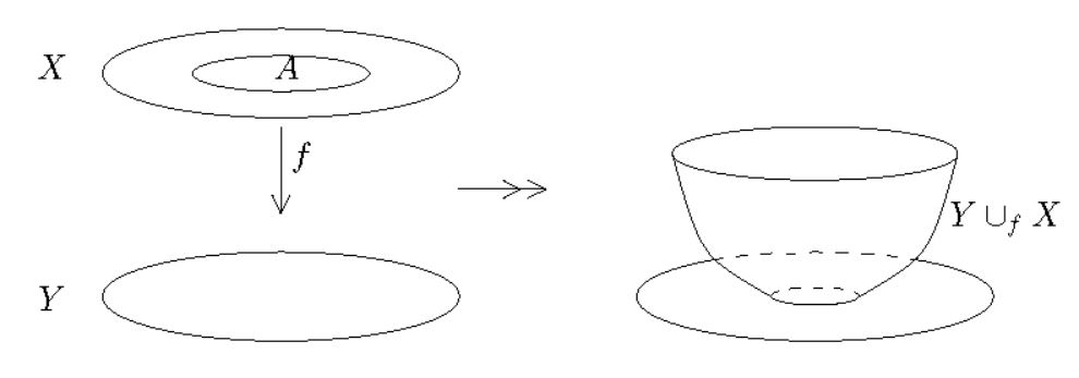
If $g$ is an topological subspace inclusion $A \subset X$, then in topology its pushout along $f$ is traditionally written as

$$X \cup_f Y \;\coloneqq\; (X, \tau_X) \underset{(A, \tau_A)}{\sqcup} (Y, \tau_Y)$$

and called the attachment space (sometimes: attaching space or adjunction space) of $A \subset X$ along $f$.

(graphics from Aguilar-Gitler-Prieto 02)

Example

(n-sphere as pushout of the equator inclusions into its hemispheres)

As an important special case of example , let

$$i_n \;\colon\; S^{n-1}\longrightarrow D^n$$

be the canonical inclusion of the standard (n-1)-sphere as the boundary of the standard n-disk (example ).

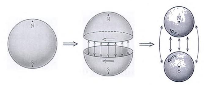
Then the colimit of topological spaces under the span diagram,

$$D^n \overset{\phantom{A} i_n \phantom{A}}{\longleftarrow} S^{n-1} \overset{\phantom{A} i_n \phantom{A}}{\longrightarrow} D^n \,,$$

is the topological n-sphere $S^n$ (example ):

$$\array{ S^{n-1} &\overset{i_n}{\longrightarrow}& D^n \\ {}^{\mathllap{i_n}}\downarrow &(po)& \downarrow \\ D^n &\longrightarrow& S^n } \,.$$

(graphics from Ueno-Shiga-Morita 95)

In generalization of this example, we have the following important concept:

Definition

(single cell attachment)

For $X$ any topological space and for $n \in \mathbb{N}$, then an $n$-cell attachment to $X$ is the result of gluing an n-disk to $X$, along a prescribed image of its bounding (n-1)-sphere (def. ):

Let

$$\phi \;\colon\; S^{n-1} \longrightarrow X$$

be a continuous function, then the space attachment (example )

$$X \cup_\phi D^n \,\in Top$$

is the topological space which is the pushout of the boundary inclusion of the $n$-sphere along $\phi$, hence the universal space that makes the following diagram commute:

$$\array{ S^{n-1} &\stackrel{\phi}{\longrightarrow}& X \\ {}^{\mathllap{\iota_n}}\downarrow &(po)& \downarrow \\ D^n &\longrightarrow& X \cup_\phi D^n } \,.$$

Example

(discrete topological spaces from 0-cell attachment to the empty space)

A single cell attachment of a 0-cell, according to example is the same as forming the disjoint union space $X \sqcup \ast$ with the point space $\ast$:

$$\array{ (S^{-1} = \emptyset) &\overset{\exists !}{\longrightarrow}& X \\ \downarrow &(po)& \downarrow \\ (D^0 = \ast) &\longrightarrow& X \sqcup \ast } \,.$$

In particular if we start with the empty topological space $X = \emptyset$ itself (example ), then by attaching 0-cells we obtain a discrete topological space. To this then we may attach higher dimensional cells.

Definition

(attaching many cells at once)

If we have a set of attaching maps $\{S^{n_i-1} \overset{\phi_i}{\longrightarrow} X\}_{i \in I}$ (as in def. ), all to the same space $X$, we may think of these as one single continuous function out of the disjoint union space of their domain spheres

$$(\phi_i)_{i \in I} \;\colon\; \underset{i \in I}{\sqcup} S^{n_i-1} \longrightarrow X \,.$$

Then the result of attaching all the corresponding $n$-cells to $X$ is the pushout of the corresponding disjoint union of boundary inclusions:

$$\array{ \underset{i \in I}{\sqcup} S^{n_i - 1} &\overset{(\phi_i)_{i \in I}}{\longrightarrow}& X \\ \downarrow &(po)& \downarrow \\ \underset{i \in I}{\sqcup} D^n &\longrightarrow& X \cup_{(\phi_i)_{i \in I}} \left(\underset{i \in I}{\sqcup} D^n\right) } \,.$$

Apart from attaching a set of cells all at once to a fixed base space, we may “attach cells to cells” in that after forming a given cell attachment, then we further attach cells to the resulting attaching space, and ever so on:

Definition

(relative cell complexes and CW-complexes)

Let $X$ be a topological space, then A topological relative cell complex of countable height based on $X$ is a continuous function

$$f \colon X \longrightarrow Y$$

and a sequential diagram of topological space of the form

$$X = X_0 \hookrightarrow X_1 \hookrightarrow X_2 \hookrightarrow X_3 \hookrightarrow \cdots$$

such that

1. each $X_k \hookrightarrow X_{k+1}$ is exhibited as a cell attachment according to def. , hence presented by a pushout diagram of the form

   $$\array{ \underset{i \in I}{\sqcup} S^{n_i - 1} &\overset{(\phi_i)_{i \in I}}{\longrightarrow}& X_k \\ \downarrow &(po)& \downarrow \\ \underset{i \in I}{\sqcup} D^{n_i} &\longrightarrow& X_{k+1} } \,.$$

2. $Y = \underset{k\in \mathbb{N}}{\cup} X_k$ is the union of all these cell attachments, and $f \colon X \to Y$ is the canonical inclusion; or stated more abstractly: the map $f \colon X \to Y$ is the inclusion of the first component of the diagram into its colimiting cocone $\underset{\longrightarrow}{\lim}_k X_k$:

   $$\array{ X = X_0 &\longrightarrow& X_1 &\longrightarrow& X_2 &\longrightarrow& \cdots \\ & {}_{\mathllap{f}}\searrow & \downarrow & \swarrow && \cdots \\ && Y = \underset{\longrightarrow}{\lim} X_\bullet }$$

If here $X = \emptyset$ is the empty space then the result is a map $\emptyset \hookrightarrow Y$, which is equivalently just a space $Y$ built form “attaching cells to nothing”. This is then called just a topological cell complex of countable height.

Finally, a topological (relative) cell complex of countable height is called a CW-complex is the $(k+1)$-st cell attachment $X_k \to X_{k+1}$ is entirely by $(k+1)$-cells, hence exhibited specifically by a pushout of the following form:

$$\array{ \underset{i \in I}{\sqcup} S^{k} &\overset{(\phi_i)_{i \in I}}{\longrightarrow}& X_k \\ \downarrow &(po)& \downarrow \\ \underset{i \in I}{\sqcup} D^{k+1} &\longrightarrow& X_{k+1} } \,.$$

Given a CW-complex, then $X_n$ is also called its $n$-skeleton.

A finite CW-complex is one which admits a presentation in which there are only finitely many attaching maps, and similarly a countable CW-complex is one which admits a presentation with countably many attaching maps.

$\,$

Subspaces

We discuss special classes of subspaces of topological spaces that play an important role in the theory, in particular for the discussion of topological manifolds below:

1. Connected components

2. Embeddings

Connected components

Via homeomorphism to disjoint union spaces one may characterize whether topological spaces are connected (def. below), and one may decompose every topological space into its connected components (def. below).

The important subtlety in to beware of is that a topological space is not in general the disjoint union space of its connected components. The extreme case of this phenomenon are totally disconnected topological spaces (def. below) which are nevertheless not discrete (examples and below). Spaces which are free from this exotic behaviour include the locally connected topological spaces (def. below) and in particular the locally path-connected topological spaces (def. below).

Definition

(connected topological space)

A topological space $(X,\tau)$ (def. ) is called connected if the following equivalent conditions hold:

1. For all pairs of topological spaces $(X_1, \tau_1), (X_2, \tau_2)$ such that $(X, \tau)$ is homeomorphic (def. ) to their disjoint union space (def. )

   $$(X,\tau) \simeq (X_1,\tau_1) \sqcup (X_2,\tau_2)$$

   then exactly one of the two spaces is the empty space (example ).

2. For all pairs of open subsets $U_1, U_2 \subset X$ if

   $$U_1 \cup U_2 = X \phantom{A}\text{and} \phantom{A} U_1 \cap U_2 = \emptyset$$

   then exactly one of the two subsets is the empty set;

3. if a subset $CO \subseteq X$ is both an open subset and a closed subset (def. ) then $CO = X$ if and only if $CO$ is non-empty.

Lemma

The conditions in def. are indeed equivalent.

Proof

First consider the equivalence of the first two statements:

Suppose that in every disjoint union decomposition of $(X,\tau)$ exactly one summand is empty. Now consider two disjoint open subsets $U_1, U_2 \subset X$ whose union is $X$ and whose intersection is empty. We need to show that exactly one of the two subsets is empty.

Write $(U_1, \tau_{1})$ and $(U_2, \tau_2)$ for the corresponding topological subspaces. Then observe that from the definition of subspace topology (example ) and of the disjoint union space (example ) we have a homeomorphism

$$X \simeq (U_1, \tau_1) \sqcup (U_2, \tau_2)$$

because by assumption every open subset $U \subset X$ is the disjoint union of open subsets of $U_1$ and $U_2$, respectively:

$$U = U \cap X = U \cap (U_1 \sqcup U_2) = (U \cap U_1) \sqcup (U \cap U_2) \,,$$

which is the definition of the disjoint union topology.

Hence by assumption exactly one of the two summand spaces is the empty space and hence the underlying set is the empty set.

Conversely, suppose that for every pair of open subsets $U_1, U_2 \subset U$ with $U_1 \cup U_2 = X$ and $U_1 \cap U_2 = \emptyset$ then exactly one of the two is empty. Now consider a homeomorphism of the form $(X,\tau) \simeq (X_1, \tau_1) \sqcup (X_2,\tau_2)$. By the nature of the disjoint union space this means that $X_1, X_2 \subset X$ are disjoint open subsets of $X$ which cover $X$. So by assumption precisely one of the two subsets is the empty set and hence precisely one of the two topological spaces is the empty space.

Now regarding the equivalence to the third statement:

If a subset $CO \subset X$ is both closed and open, this means equivalently that it is open and that its complement $X \setminus CO$ is also open, hence equivalently that there are two open subsets $CO, X \backslash CO \subset X$ whose union is $X$ and whose intersection is empty. This way the third condition is equivalent to the second, hence also to the first.

Remark

(empty space is not connected)

According to def. the empty topological space $\emptyset$ (def. ) is not connected, since $\emptyset \simeq \emptyset \sqcup \emptyset$, where both instead of exactly one of the summands are empty.

Of course it is immediate to change def. so that it would regard the empty space as connected. This is a matter of convention.

Example

(connected subspaces of the real line are the intervals)

Regard the real line with its Euclidean metric topology (example , ). Then a subspace $S \subset \mathbb{R}$ (example ) is connected (def. ) precisely if it is an interval, hence precisely if

$$\underset{x,y \in S \subset \mathbb{R}}{\forall} \underset{ r \in \mathbb{R} }{\forall} \left( \left( x \lt r \lt y \right) \Rightarrow \left( r \in S \right) \right) \,.$$

Proof

Suppose on the contrary that we had $x \lt r \lt y$ but $r \notin S$. Then by the nature of the subspace topology there would be a decomposition of $S$ as a disjoint union of disjoint open subsets:

$$S = \left( S \cap (r,\infty) \right) \sqcup \left( S \cap (-\infty,r) \right) \,.$$

But since $x \lt r$ and $r \lt y$ both these open subsets were non-empty, thus contradicting the assumption that $S$ is connected. This yields a proof by contradiction.

Proposition

(continuous images of connected spaces are connected)

Let $X$ be a connected topological space (def. ), let $Y$ be any topological space, and let

$$f \;\colon\; X \longrightarrow Y$$

be a continuous function (def. ). This factors via continuous functions through the image

$$f \;\colon\; X \underoverset{surjective}{p}{\longrightarrow} f(X) \underoverset{injective}{i}{\longrightarrow} Y$$

for $f(X)$ equipped either with he subspace topology relative to $Y$ or the quotient topology relative to $X$ (example ). In either case:

If $X$ is a connected topological space (def. ), then so is $f(X)$.

In particular connectedness is a topological property (def. ).

Proof

Let $U_1,U_2 \subset f(X)$ be two open subsets such that $U_1 \cup U_2 = f(X)$ and $U_1 \cap U_2 = \emptyset$. We need to show that precisely one of them is the empty set.

Since $p$ is a continuous function, also the pre-images $p^{-1}(U_1), p^{-1}(U_2) \subset X$ are open subsets and are still disjoint. Since $p$ is surjective it also follows that $p^{-1}(U_1) \cup p^{-1}(U_2) = X$. Since $X$ is connected, it follows that one of these two pre-images is the empty set. But again sicne $p$ is surjective, this implies that precisely one of $U_1, U_2$ is empty, which means that $f(X)$ is connected.

This yields yet another quick proof via topology of a classical fact of analysis:

Corollary

(intermediate value theorem)

Regard the real numbers $\mathbb{R}$ with their Euclidean metric topology (example , example ), and consider a closed interval $[a,b] \subset \mathbb{R}$ (example ) equipped with its subspace topology (example ).

Then a continuous function (def. )

$$f \colon [a,b] \longrightarrow \mathbb{R}$$

takes every value in between $f(a)$ and f(b).

Proof

By example the interval $[a,b]$ is connected. By prop. also its image $f([a,b]) \subset \mathbb{R}$ is connected. By example that image is hence itself an interval. This implies the claim.

Example

(product space of connected spaces is connected)

Let $\{X_i\}_{i \in I}$ be a set of connected topological spaces (def. ). Then also their product topological space $\underset{i \in I}{\prod}X_i$ (example ) is connected.

Proof

Let $U_1, U_2 \subset \underset{i \in I}{\prod}X_i$ be an open cover of the product space by two disjoint open subsets. We need to show that precisely one of the two is empty. Since each $X_i$ is connected and hence non-empty, the product space is not empty, and hence it is sufficient to show that at least one of the two is empty.

Assume on the contrary that both $U_1$ and $U_2$ were non-empty.

Observe first that if so, then we could find $x_1 \in U_1$ and $x_2 \in U_2$ whose coordinates differed only in a finite subset of $I$. This is since by the nature of the Tychonoff topology $\pi_i(U_1) = X_i$ and $\pi_i(U_2) = X_i$ for all but a finite number of $i \in i$.

Next observe that we then could even find $x'_1 \in U_1$ that differed only in a single coordinate from $x_2$: Because pick one coordinate in which $x_1$ differs from $x_2$ and change it to the corresponding coordinate of $x_2$. Since $U_1$ and $U_2$ are a cover, the resulting point is either in $U_1$ or in $U_2$. If it is in $U_2$, then $x_1$ already differed in only one coordinate from $x_2$ and we may take $x'_1 \coloneqq x_1$. If instead the new point is in $U_1$, then rename it to $x_1$ and repeat the argument. By induction this finally yields an $x'_1$ as claimed.

Therefore it is now sufficient to see that it leads to a contradiction to assume that there are points $x_1 \in U_1$ and $x_2 \in U_2$ that differ in only the $i_0$th coordinate, for some $i_0 \in I$, in that this would imply that $x_1 = x_2$.

Observe that the inclusion

$$\iota \colon X_{i_0} \longrightarrow \underset{i \in I}{\prod} X_i$$

which is the identity on the $i_0$th component and is otherwise constant on the $i$th component of $x_1$ or equivalently of $x_2$ is a continuous function, by the nature of the Tychonoff topology (example ).

Therefore also the restrictions $\iota^{-1}(U_1)$ and $\iota^{-1}(U_2)$ are open subsets. Moreover they are still disjoint and cover $X_{i_0}$. Hence by the connectedness of $X_{i_0}$, precisely one of them is empty. This means that the $i_0$-component of both $x_1$ and $x_2$ must be in the other subset of $X_i$, and hence that $x_1$ and $x_2$ must both be in $U_1$ or both in $U_2$, contrary to the assumption.

$\,$

While topological spaces are not always connected, they always decompose at least as sets into their connected components:

Definition

(connected components)

For $(X,\tau)$ a topological space, then its connected components are the equivalence classes under the equivalence relation on $X$ which regards two points as equivalent if they both sit in some subset which, as a topological subspace (example ), is connected (def. ):

$$(x \sim y) \;\coloneqq\; \left( \underset{ U \subset X }{\exists} \left( \left( x,y \in U \right) \phantom{A}\text{and}\phantom{A} \left( U \, \text{is connected} \right) \right) \right) \,.$$

Equivalently, the connected components are the maximal elements in the pre-ordered set of connected subspaces, pre-ordered by inclusion.

Example

(connected components of disjoint union spaces)

For $\{X_i\}_{i \in I}$ an $I$-indexed set of connected topological spaces, then the set of connected components (def. ) of their disjoint union space $\underset{i \in I}{\sqcup}X_i$ (example ) is the index set $I$.

In general the situation is more complicated than in example , this we come to in examples and below. But first notice some basic properties of connected components:

Proposition

(topological closure of connected subspace is connected)

Let $(X,\tau)$ be a topological space and let $S \subset X$ be a subset which, as a subspace, is connected (def. ). Then also the topological closure $Cl(S) \subset X$ is connected

Proof

Suppose that $Cl(S) = A \sqcup B$ with $A,B \subset X$ disjoint open subsets. We need to show that one of the two is empty.

But also the intersections $A \cap S\,,B \cap S \subset S$ are disjoint subsets, open as subsets of the subspace $S$ with $S = (A \cap S) \sqcup (B \cap S)$. Hence by the connectedness of $S$, one of $A \cap S$ or $B \cap S$ is empty. Assume $B \cap S$ is empty, otherwise rename. Hence $A \cap S = S$, or equivalently: $S \subset A$. By disjointness of $A$ and $B$ this means that $S \subset Cl(S) \setminus B$. But since $B$ is open, $Cl(S) \setminus B$ is still closed, so that

$$(S \subset Cl(S) \setminus B) \Rightarrow (Cl(S) \subset Cl(S) \setminus B) \,.$$

This means that $B = \emptyset$, and hence that $Cl(S)$ is connected.

Proposition

(connected components are closed)

Let $(X,\tau)$ be a topological space. Then its connected components (def. ) are closed subsets.

Proof

By definition, the connected components are maximal elements in the set of connected subspaces pre-ordered by inclusion. Assume a connected component $U$ were not closed. By prop. its closure $Cl(U)$ is still closed, and would be strictly larger, contradicting the maximality of $U$. This yields a proof by contradiction.

Remark

Prop. implies that when a space has a finite set of connected components, then they are not just closed but also open, hence clopen subsets (because then each is the complement of a finite union of closed subspaces). This in turn means that the space is the disjoint union space of its connected components.

For a non-finite set of connected components this remains true if the space is locally connected see def. , lemma below.

$\,$

We now highlight the subtlety that not every topological space is the disjoint union of its connected components. For this it is useful to consider the following extreme situation:

Definition

(totally disconnected topological space)

A topological space is called totally disconnected if all its connected components (def. ) are singletons, hence point spaces (example ).

The trivial class of examples is this:

Example

(discrete topological spaces are totally disconnected)

Every discrete topological space (example ) is a totally disconnected topological space (def. ).

But the important point is that there are non-discrete totally disconnected topological spaces:

Example

(the rational numbers are totally disconnected but non-discrete topological space)

The rational numbers $\mathbb{Q} \subset \mathbb{R}$ equipped with their subspace topology (def. ) inherited from the Euclidean metric topology (example , example ) on the real numbers, form a totally disconnected space (def. ), but not a discrete topological space (example ).

Proof

It is clear that the subspace topology is not discrete, since the singletons $\{q\} \subset \mathbb{Q}$ are not open subsets (because their pre-image in $\mathbb{R}$ are still singletons, and the points in a metric space are closed, by example and prop. ).

What we need to see is that $\mathbb{Q} \subset \mathbb{R}$ is nevertheless totally disconnected:

By construction, a base for the topology (def. ) is given by the open subsets which are restrictions of open intervals of real numbers to the rational numbers

$$(a,b)_{\mathbb{Q}} \coloneqq (a,b) \cap \mathbb{Q}$$

for $a \lt b \in \mathbb{R}$.

Now for any such $a \lt b$ there exists an irrational number $r \in \mathbb{R}\backslash \mathbb{Q}$ with $a \lt r \lt b$. This being irrational implies that $(a,r)_{\mathbb{Q}} \subset \mathbb{Q}$ and $(r,b)_{\mathbb{Q}} \subset \mathbb{Q}$ are disjoint subsets. Therefore every basic open subset is the disjoint union of (at least) two open subsets:

$$(a,b)_{\mathbb{Q}} = (a,r)_{\mathbb{Q}} \cup (r,b)_{\mathbb{Q}} \,.$$

Hence no non-empty open subspace of the rational numbers is connected.

Example

(Cantor space is totally disconnected but non-discrete)

The Cantor space $\underset{n \in \mathbb{N}}{\prod} Disc(\{0,1\})$ (example ) is a totally disconnected topological space (def. ) but is not a discrete topological space.

Proof

The base opens (def. ) of the product topological space $\underset{n \in \mathbb{N}}{\prod} Disc(\{1,2\})$ (example ) are of the form

$$\left( \underset{i \in I \subset \mathbb{N}}{\prod} U_i \right) \times \left( \underset{k \in \mathbb{N}\setminus I}{\prod} \{1,2\} \right) \,.$$

for $I \subset \mathbb{N}$ a finite subset.

First of all this is not the discrete topology, for that also contains infinite products of proper subsets of $\{1,2\}$ as open subsets, hence is strictly finer.

On the other hand, since $I \subset \mathbb{N}$ is finite, $\mathbb{N}\setminus I$ is non-empty and hence there exists some $k_0 \in \mathbb{N}$ such that the corresponding factor in the above product is the full set $\{1,2\}$. But then the above subset is the disjoint union of the open subsets

$$\{1\}_{k_0} \times \left( \underset{i \in I \setminus \{k_0\} \subset \mathbb{N}}{\prod} U_i \right) \times \left( \underset{k \in \mathbb{N}\setminus (I \cup \{k_0\}) }{\prod} \{1,2\} \right) \phantom{AAA} \text{and} \phantom{AAA} \{2\}_{k_0} \times \left( \underset{i \in I \setminus \{k_0\} \subset \mathbb{N}}{\prod} U_i \right) \times \left( \underset{k \in \mathbb{N}\setminus (I\setminus \k_0 ) }{\prod} \{1,2\} \right) \,.$$

In particular if $x \neq y$ are two distinct points in the original open subset, them being distinct means that there is a smallest $k_0 \in \mathbb{N}$ such that they have different coordinates in $\{1,2\}$ in that position. By the above this implies that they belong to different connected components.

In applications to geometry (such as in the definition of topological manifolds below) one is typically interested in topological spaces which do not share the phenomenon of examples or , hence which are the disjoint union of their connected components:

Definition

(locally connected topological spaces)

A topological space $(X,\tau)$ is called locally connected if the following equivalent conditions hold:

1. For every point $x$ and every neighbourhood $U_x \supset \{x\}$ there is a connected (def. ) open neighbourhood $Cn_x \subset U_x$.

2. Every connected component of every open subspace of $X$ is open.

3. Every open subspace (example ) is the disjoint union space (def. ) of its connected components (def. ).

Lemma

The conditions in def. are indeed all equivalent.

Proof

$\,$

1) $\Rightarrow$ 2)

Assume every neighbourhood of $X$ contains a connected neighbourhood and let $U \subset X$ be an open subset with $U_0 \subset U$ a connected component. We need to show that $U_0$ is open.

Consider any point $x \in U_0$. Since then also $x \in U$, there is a connected open neighbourhood $U_{x,0}$ of $x$ in $X$. Observe that this must be contained in $U_0$, for if it were not then $U_0 \cup U_{x,0}$ were a larger open connected open neighbourhood, contradicting the maximality of the connected component $U_0$.

Hence $U_0 = \underset{x \in U_0}{\cup} U_{x,0}$ is a union of open subsets, and hence itself open.

2) $\Rightarrow$ 3)

Now assume that every connected component of every open subset $U$ is open. Since the connected components generally constitute a cover of $X$ by disjoint subsets, this means that now they form an open cover by disjoint subsets. But by forming intersections with the cover this implies that every open subset of $U$ is the disjoint union of open subsets of the connected components (and of course every union of open subsets of the connected components is still open in $U$), which is the definition of the topology on the disjoint union space of the connected components.

3) $\Rightarrow$ 1)

Finally assume that every open subspace is the disjoint union of its connected components. Let $x$ be a point and $U_x \supset \{x\}$ a neighbourhood. We need to show that $U_x$ contains a connected neighbourhood of $x$.

But, by definition, $U_x$ contains an open neighbourhood of $x$ and by assumption this decomposes as the disjoint union of its connected components. One of these contains $x$. Since in a disjoint union space all summands are open, this is the required connected open neighbourhood.

Example

(Euclidean space is locally connected)

For $n \in \mathbb{N}$ the Euclidean space $\mathbb{R}^n$ (example ) (with its metric topology, example ) is locally connected (def. ).

Proof

By nature of the Euclidean metric topology, every neighbourhood $U_x$ of a point $x$ contains an open ball containing $x$ (def. ). Moreover, every open ball clearly contains an open cube, hence a product space $\underset{i \in \{1, \cdots, n\}}{\prod} (x_i-\epsilon, x_i + \epsilon)$ of open intervals which is still a neighbourhood of $x$ (example ).

Now intervals are connected by example and product spaces of connected spaces are connected by example . This shows that ever open neighbourhood contains a connected neighbourhood, which is the characterization of local connectedness in the first item of def. .

Proposition

(open subspace of locally connected space is locally connected)

Every open subspace (example ) of a locally connected topological space (example ) is itself locally connected

Proof

This is immediate from the first item of def. .

$\,$

Another important class of examples of locally connected topological spaces are topological manifolds, this we discuss as prop. below.

$\,$

There is also a concept of connectedness which is “geometric” instead of “purely topological” by definition:

Definition

(path)

Let $X$ be a topological space. Then a path or continuous curve in $X$ is a continuous function

$$\gamma \;\colon\; [0,1] \longrightarrow X$$

from the closed interval (example ) equipped with its Euclidean metric topology (example , example ).

We say that this path connects its endpoints $\gamma(0), \gamma(1) \in X$.

The following is obvious, but the construction is important:

Lemma

(being connected by a path is equivalence relation)

Let $(X,\tau)$ be a topological space. Being connected by a path (def. ) is an equivalence relation $\sim_{pcon}$ on the underlying set of points $X$.

Proof

We need to show that the relation is reflexive, symmetric and transitive.

For $x \in X$ a point, then the constant function with value $x$

$$const_x \;\colon\; [0,1] \to \ast \overset{}{\longrightarrow} X$$

is continuous (example ). Therefore $x \sim_{pcon} x$ for all points (reflexivity).

For $x,y \in X$ two points and

$$\gamma \;\colon\; [0,1] \longrightarrow X$$

a path connecting them, then the reverse path

$$[0,1] \overset{(1-(-))}{\longrightarrow} [0,1] \overset{\gamma}{\longrightarrow} X$$

is continuous (the function $[0,1] \overset{1-(-)}{\to} [0,1]$ is continuous because polynomials are continuous ). Hence with $x \sim_{pcon} y$ also $y \sim_{pcon} x$ (symmetry).

For $x,y,z \in X$ three points and for

$$\gamma_1, \gamma_2 \;\colon\; [0,1] \longrightarrow X$$

two paths with $\gamma_1(0) = x$, $\gamma_1(1) = \gamma_2(0) = y$ and $\gamma_2(1) = z$

$$\gamma_1(x) \overset{\pahntom{A}\gamma_1\phantom{A}}{\rightsquigarrow} \gamma_1(1) = \gamma_2(0) \overset{ \phantom{A}\gamma_2\phantom{A} }{\rightsquigarrow} \gamma_2(1)$$

consider the function

$$\array{ [0,1] &\overset{ (\gamma_2 \cdot \gamma_1) }{\longrightarrow}& X \\ t &\mapsto& \mathrlap{ \left\{ \array{ \gamma_1(2t) & \vert& 0 \leq t \leq 1/2 \\ \gamma_2(2t-1) &\vert& 1/2 \leq t \leq 1 } \right. } } \,.$$

This is a continuous function by example , hence this constitutes a path connecting $x$ with $z$ (the “concatenated path”). Therefore $x \sim_{pcon} y$ and $y \sim_{pcon} z$ implies $x \sim_{pcon} z$ (transitivity).

Definition

(path-connected components)

Let $X$ be a topological space. The equivalence classes of the equivalence relation “connected by a path” (def. , lemma ) are called the path-connected components of $X$. The set of the path-connected components is usually denoted

$$\pi_0(X) \;\coloneqq\; X/\sim_{pcon} \,.$$

(The notation reflects the fact that this is the degree-zero case of a more general concept of homotopy groups $\pi_n$ for all $n \in \mathbb{N}$. We discuss the fundamental group $\pi_1$ in part 2. The higher homotopy groups are discussed in Introduction to Homotopy Theory).

If there is a single path-connected component ($\pi_0(\ast) \simeq \ast$), then $X$ is called a path-connected topological space.

Example

(Euclidean space is path-connected)

For $n \in \mathbb{N}$ then Euclidean space $\mathbb{R}^n$ is a path-connected topological space (def. ).

Because for $\vec x, \vec y \in \mathbb{R}^n$, consider the function

$$\array{ [0,1] &\overset{\gamma}{\longrightarrow}& \mathbb{R}^n \\ t &\mapsto& t \vec y + (1-t) \vec x } \,.$$

This clearly has the property that $\gamma(0) = \vec x$ and $\gamma(1) = \vec y$. Moreover, it is a polynomial function and polynomials are continuous functions (example ).

Example

(continuous image of path-connected space is path-connected)

Let $X$ be a path-connected topological space and let

$$f \colon X \longrightarrow Y$$

be a continuous function. Then also the image $f(X)$ of $X$

$$X \underoverset{\text{surjective}}{p}{\longrightarrow} f(X) \underoverset{\text{injective}}{i}{\longrightarrow} Y$$

with either of its two possible topologies (example ) is path-connected.

In particular path-connectedness is a topological property (def. ).

Proof

Let $x,y \in X$ be two points. Since $p \;\colon\; X \to f(X)$ is surjective, there are pre-images $p^{-1}(x), p^{-1}(y) \in X$. Since $X$ is path-connected, there is a continuous function

$$\gamma \colon [0,1] \longrightarrow X$$

with $\gamma(0) = p^{-1}(x)$ and $\gamma(1) = p^{-1}(y)$. Since the composition of continuous functions is continuous, it follows that $p \circ \gamma \;\colon\; [0,1] \to f(X)$ is a path connecting $x$ with $y$.

Remark

(path space)

Let $X$ be a topological space. Since the interval $[0,1]$ is a locally compact topological space (example ) there is the mapping space

$$P X \;\coloneqq\; Maps([0,1],X)$$

hence the set of paths in $X$ (def. ) equipped with the compact-open topology (def. ).

This is often called the path space of $X$.

By functoriality of the mapping space (remark ) the two endpoint inclusions

$$\ast \overset{const_0}{\hookrightarrow} [0,1] \phantom{AA} \text{and} \phantom{AA} \ast \overset{const_1}{\hookrightarrow} [0,1]$$

induce two continuous functions of the form

$$P X = Maps([0,1],X) \underoverset {\underset{const_1^\ast}{\longrightarrow}} {\overset{const_0^\ast}{\longrightarrow}} {} Maps(\ast,X) \simeq X \,.$$

The coequalizer (example ) of these two functions is the set $\pi_0(X)$ of path-connected components (def. ) topologized with the corresponding final topology (def. ).

Lemma

(path-connected spaces are connected)

A path connected topological space $X$ (def. ) is connected (def. ).

Proof

Assume it were not, then it would be covered by two disjoint non-empty open subsets $U_1, U_2 \subset X$. But by path connectedness there were a continuous path $\gamma \colon [0,1] \to X$ from a point in one of the open subsets to a point in the other. The continuity would imply that $\gamma^{-1}(U_1), \gamma^{-1}(U_2) \subset [0,1]$ were a disjoint open cover of the interval. This would be in contradiction to the fact that intervals are connected. Hence we have a proof by contradiction.

Definition

(locally path-connected topological space)

A topological space $X$ is called locally path-connected if for every point $x \in X$ and every neighbourhood $U_x \supset \{x\}$ there exists a neighbourhood $C_x \subset U_x$ which, as a subspace, is path-connected (def. ).

Examples

(Euclidean space is locally path-connected)

For $n \in \mathbb{N}$ then Euclidean space $\mathbb{R}^n$ (with its metric topology) is locally path-connected, since each open ball is a path-connected topological space (example ).

Example

(open subspace of locally path-connected space is locally path-connected)

Every open subspace of a locally path-connected topological space is itself locally path-connected.

Another class of examples we consider below: locally Euclidean topological spaces are locally path-connected (prop. below).

Proposition

Let $X$ be a locally path-connected topological space (def. ). Then each of its path-connected components is an open set and a closed set.

Proof

To see that every path connected component $P_x$ is open, it is sufficient to show that every point $y \in P_x$ has an neighbourhood $U_y$ which is still contained in $P_x$. But by local path connectedness, $y$ has a neighbourhood $V_y$ which is path connected. It follows by concatenation of paths (as in the proof of lemma ) that $V_y \subset P_x$.

Now each path-connected component $P_x$ is the complement of the union of all the other path-connected components. Since these are all open, their union is open, and hence the complement $P_x$ is closed.

Proposition

(in a locally path-connected space connected components coincide with path-connected components)

Let $X$ be a locally path-connected topological space (def. ). Then the connected components of $X$ according to def. agree with the path-connected components according to def. .

In particular, locally path connected spaces are locally connected topological spaces (def. ).

Proof

A path connected component is always connected by lemma , and in a locally path-connected space it is also open, by prop. . This implies that the path-connected components are maximal connected subspaces, and hence must be the connected components.

Conversely let $U$ be a connected component. It is now sufficient to see that this is path-connected. Suppose it were not, then it would be covered by more than one disjoint non-empty path-connected components. But by prop. these would all be open. This would be in contradiction with the assumption that $U$ is connected. Hence we have a proof by contradiction.

$\,$

Embeddings

Often it is important to know whether a given space is homeomorphism to its image, under some continuous function, in some other space. This concept of embedding of topological spaces (def. below) we will later refine to that of embedding of smooth manifolds (below).

Definition

(embedding of topological spaces)

Let $(X,\tau_X)$ and $(Y,\tau_Y)$ be topological spaces. A continuous function $f \;\colon\; X \longrightarrow Y$ is called an embedding of topological spaces if in its image factorization (example )

$$f \;\colon\; X \overset{\phantom{A}\simeq\phantom{A}}{\longrightarrow} f(X) \overset{\phantom{AAA}}{\hookrightarrow} Y$$

with the image $f(X) \hookrightarrow Y$ equipped with the subspace topology (example ), we have that $X \to f(X)$ is a homeomorphism (def. ).

Proposition

(open/closed continuous injections are embeddings)

A continuous function $f \colon (X, \tau_X) \to (Y,\tau_Y)$ which is

1. an injective function

2. an open map or a closed map (def. )

is an embedding of topological spaces (def. ).

This is called a closed embedding if the image $f(X) \subset Y$ is a closed subset.

Proof

If $f$ is injective, then the map onto its image $X \to f(X) \subset Y$ is a bijection. Moreover, it is still continuous with respect to the subspace topology on $f(X)$ (example ). Now a bijective continuous function is a homeomorphism precisely if it is an open map or a closed map, by prop. . But the image projection of $f$ has this property, respectively, if $f$ does, by prop .

The following characterization of closed embeddings uses concepts of (locally) compact spaces discussed below. The reader may wish to skip the following and only compact back to it in the discussion of embeddings of smooth manifolds further bellow in prop. .

Proposition

(injective proper maps to locally compact spaces are equivalently the closed embeddings)

Let

1. $X$ be a topological space,

2. $Y$ a locally compact topological space (def. ),

3. $f \colon X \to Y$ a continuous function.

Then the following are equivalent:

1. $f$ is an injective proper map (prop. ),

2. $f$ is a closed embedding of topological spaces (def ).

Proof

In one direction, if $f$ is an injective proper map, then since proper maps to locally compact spaces are closed (prop. ), we have that $f$ is also closed map. The claim then follows since closed injections are embeddings (prop. ), and since the image of a closed map is closed, by definition.

Conversely, if $f$ is a closed embedding, we only need to show that the embedding map is proper. So for $C \subset Y$ a compact subspace, we need to show that the pre-image $f^{-1}(C) \subset X$ is also compact. But since $f$ is an injection (being an embedding), that pre-image is equivalently just the intersection $f^{-1}(C) \simeq C \cap f(X) \subset Y$, regarded as a subspace of $Y$.

To see that this is compact, let $\{V_i \subset X\}_{i \in I}$ be an open cover of the subspace $C \cap f(X)$, hence, by the nature of the subspace topology, let $\{U_i \subset Y\}_{i \in I}$ be a set of open subsets of $Y$, which cover $C \cap f(X) \subset Y$ and with $V_i$ the restriction of $U_i$ to $C \cap f(X)$. Now since $f(X) \subset Y$ is closed by assumption, it follows that the complement $Y \setminus f(X)$ is open and hence that

$$\{ U_i \subset Y \}_{i \in I} \sqcup \{ Y \setminus f(X) \}$$

is an open cover of $C \subset Y$. By compactness of $C$ this has a finite subcover. Since restricting that finite subcover back to $C \cap f(X)$ makes the potential element $Y \setminus f(X)$ disappear, this restriction is a finite subcover of $\{V_i \subset C \cap f(X)\}$. This shows that $C \cap f(X)$ is compact.

$\,$

Compact spaces

We discuss compact topological spaces (def below), the generalization of compact metric spaces above. Compact spaces are in some sense the “small” objects among topological spaces, analogous in topology to what finite sets are in set theory, or what finite-dimensional vector spaces are in linear algebra, and equally important in the theory.

$\,$

Prop. suggests the following simple definition :

Definition

(open cover)

An open cover of a topological space $(X,\tau)$ (def. ) is a set $\{U_i \subset X\}_{i \in I}$ of open subsets $U_i$ of $X$, indexed by some set $I$, such that their union is all of $X$: $\underset{i \in I}{\cup} U_i \;=\; X$.

A subcover of a cover is a subset $J \subset I$ such that $\{U_i \subset X\}_{i \in J \subset I}$ is still a cover.

Definition

(compact topological space)

A topological space $X$ (def. ) is called a compact topological space if every open cover $\{U_i \subset X\}_{i \in I}$ (def. ) has a finite subcover in that there is a finite subset $J \subset I$ such that $\{U_i \subset X\}_{i \in J}$ is still a cover of $X$ in that also $\underset{i \in J}{\cup} U_i = X$.

Remark

(varying terminology regarding “compact”)

Beware the following terminology issue which persists in the literature:

Some authors use “compact” to mean “Hausdorff and compact”. To disambiguate this, some authors (mostly in algebraic geometry, but also for instance Waldhausen) say “quasi-compact” for what we call “compact” in def. .

There are several equivalent reformulations of the compactness condition. An immediate reformulation is prop. , a more subtle one is prop. further below.

Proposition

(compactness in terms of closed subsets)

Let $(X,\tau)$ be a topological space. Then the following are equivalent:

1. $(X,\tau)$ is compact in the sense of def. .

2. Let $\{C_i \subset X\}_{i \in I}$ be a set of closed subsets (def. ) such that their intersection is empty $\underset{i \in I}{\cap} C_i = \emptyset$, then there is a finite subset $J \subset I$ such that the corresponding finite intersection is still empty $\underset{i \in J \subset i}{\cap} C_i = \emptyset$.

3. Let $\{C_i \subset X\}_{i \in I}$ be a set of closed subsets (def. ) such that it enjoys the finite intersection property, meaning that for every finite subset $J \subset I$ then the corresponding finite intersection is non-empty $\underset{i \in J \subset I}{\cap} C_i \neq \emptyset$. Then also the total intersection is non-empty, $\underset{i \in I}{\cap} C_i \neq \emptyset$.

Proof

The equivalence between the first and the second statement is immediate from the definitions after expressing open subsets as complements of closed subsets $U_i = X \setminus C_i$ and applying de Morgan's law (prop. ).

We discuss the equivalence between the first and the third statement:

In one direction, assume that $(X,\tau)$ is compact in the sense of def. , and that $\{C_i \subset X\}_{i \in I}$ satisfies the finite intersection property. We need to show that then $\underset{i \in I}{\cap} C_i \neq \emptyset$.

Assume that this were not the case, hence assume that $\underset{i \in I}{\cap} C_i = \emptyset$. This would imply that the open complements were an open cover of $X$ (def. )

$$\left\{ U_i \coloneqq X \setminus C_i \right\}_{i \in I} \,,$$

because (using de Morgan's law, prop. )

$$\begin{aligned} \underset{i \in I}{\cup} U_i\; & \coloneqq \underset{i \in I}{\cup} X \setminus C_i \\ & = X \setminus \left( \underset{i \in I}{\cap}C_i \right) \\ & = X \setminus \emptyset \\ & = X \end{aligned} \,.$$

But then by compactness of $(X,\tau)$ there were a finite subset $J \subset I$ such that $\{ U_i \subset X\}_{i \in J \subset I}$ were still an open cover, hence that $\underset{i \in J \subset I}{\cup} U_i = X$. Translating this back through the de Morgan's law again this would mean that

$$\begin{aligned} \emptyset & = X \setminus \left( \underset{i \in J \subset I}{\cup} U_i \right) \\ & \coloneqq X \setminus \left( \underset{i \in J \subset I}{\cup} X \setminus C_i \right) \\ & = \underset{i \in J \subset I}{\cap} X \setminus \left( X \setminus C_i\right) \\ & = \underset{i \in J \subset I}{\cap} C_i \,. \end{aligned}$$

This would be in contradiction with the finite intersection property of $\{C_i \subset X\}_{i \in I}$, and hence we have proof by contradiction.

Conversely, assume that every set of closed subsets in $X$ with the finite intersection property has non-empty total intersection. We need to show that the every open cover $\{U_i \subset X\}_{i \in I}$ of $X$ has a finite subcover.

Write $C_i \coloneqq X \setminus U_i$ for the closed complements of these open subsets.

Assume on the contrary that there were no finite subset $J \subset I$ such that $\underset{i \in J \subset I}{\cup} U_i = X$, hence no finite subset such that $\underset{i \in J \subset I}{\cap} C_i = \emptyset$. This would mean that $\{C_i \subset X\}_{i \in I }$ satisfied the finite intersection property.

But by assumption this would imply that $\underset{i \in I}{\cap} C_i \neq \emptyset$, which, again by de Morgan, would mean that $\underset{i \in I}{\cup} U_i \neq X$. But this contradicts the assumption that the $\{U_i \subset X\}_{i \in I}$ are a cover. Hence we have a proof by contradiction.

Example

(finite discrete spaces are compact)

A discrete topological space (def. ) is compact (def. ) precisely if its underlying set is a finite set.

Example

(closed intervals are compact topological spaces)

For any $a \lt b \in \mathbb{R}$ the closed interval (example )

$$[a,b] \subset \mathbb{R}$$

regarded with its subspace topology of Euclidean space (example ) with its metric topology (example ) is a compact topological space (def. ).

Proof

Since all the closed intervals are homeomorphic (by example ) it is sufficient to show the statement for $[0,1]$. Hence let $\{U_i \subset [0,1]\}_{i \in I}$ be an open cover (def. ). We need to show that it has an open subcover.

Say that an element $x \in [0,1]$ is admissible if the closed sub-interval $[0,x]$ is covered by finitely many of the $U_i$. In this terminology, what we need to show is that $1$ is admissible.

Observe from the definition that

1. 0 is admissible,

2. if $y \lt x \in [0,1]$ and $x$ is admissible, then also $y$ is admissible.

This means that the set of admissible $x$ forms either

1. an open interval $[0,g)$

2. or a closed interval $[0,g]$,

for some $g \in [0,1]$. We need to show that the latter is true, and for $g = 1$. We do so by observing that the alternatives lead to contradictions:

1. Assume that the set of admissible values were an open interval $[0,g)$. Pick an $i_0 \in I$ such that $g \in U_{i_0}$ (this exists because of the covering property). Since such $U_{i_0}$ is an open neighbourhood of $g$, there is a positive real number $\epsilon$ such that the open ball $B^\circ_g(\epsilon) \subset U_{i_0}$ is still contained in the patch. It follows that there is an element $x \in B^\circ_g(\epsilon) \cap [0,g) \subset U_{i_0} \cap [0,g)$ and such that there is a finite subset $J \subset I$ with $\{U_i \subset [0,1]\}_{i \in J \subset I}$ a finite open cover of $[0,x)$. It follows that $\{U_i \subset [0,1]\}_{i \in J \subset I} \sqcup \{U_{i_0}\}$ were a finite open cover of $[0,g]$, hence that $g$ itself were still admissible, in contradiction to the assumption.

2. Assume that the set of admissible values were a closed interval $[0,g]$ for $g \lt 1$. By assumption there would then be a finite set $J \subset I$ such that $\{U_i \subset [0,1]\}_{i \in J \subset I}$ were a finite cover of $[0,g]$. Hence there would be an index $i_g \in J$ such that $g \in U_{i_g}$. But then by the nature of open subsets in the Euclidean space $\mathbb{R}$, this $U_{i_g}$ would also contain an open ball $B^\circ_g(\epsilon) = (g-\epsilon, g + \epsilon)$. This would mean that the set of admissible values includes the open interval $[0,g+ \epsilon)$, contradicting the assumption.

This gives a proof by contradiction.

In contrast:

Nonexample

(Euclidean space is non-compact)

For all $n \in \mathbb{N}$, $n \gt 0$, the Euclidean space $\mathbb{R}^n$ (example ), regarded with its metric topology (example ), is not a compact topological space (def. ).

Proof

Pick any $\epsilon \in (0,1/2)$. Consider the open cover of $\mathbb{R}^n$ given by

$$\left\{ U_n \coloneqq (n-\epsilon, n+1+\epsilon) \times \mathbb{R}^{n-1} \;\subset\; \mathbb{R}^{n+1} \right\}_{n \in \mathbb{Z}} \,.$$

This is not a finite cover, and removing any one of its patches $U_n$, it ceases to be a cover, since the points of the form $(n + \epsilon, x_2, x_3, \cdots, x_n)$ are contained only in $U_n$ and in no other patch.

Below we prove the Heine-Borel theorem (prop. ) which generalizes example and example .

Example

(unions and intersection9] of [[compact spaces?)

Let $(X,\tau)$ be a topological space and let

$$\{K_i \subset X\}_{i \in I}$$

be a set of compact subspaces.

1. If $I$ is a finite set, then the union $\underset{i \in I}{\cup} K_i \subset X$ is itself a compact subspace;

2. If all $K_i \subset X$ are also closed subsets then their intersection $\underset{i \in I}{\cap} K_i \subset X$ is itself a compact subspace.

Example

(complement of compact by open subspaces is compact)

Let $X$ be a topological space. Let

1. $K\subset X$ be a compact subspace;

2. $U \subset X$ be an open subset.

Then the complement

$$K \setminus U \subset X$$

is itself a compact subspace.

In analysis, the extreme value theorem (example below) asserts that a real-valued continuous function on the bounded closed interval (def. ) attains its maximum and minimum. The following is the generalization of this statement to general topological spaces, cast in terms of the more abstract concept of compactness from def. :

Lemma

(continuous surjections out of compact spaces have compact codomain)

Let $f \colon (X,\tau_X) \longrightarrow (Y,\tau_Y)$ be a continuous function between topological spaces such that

1. $(X,\tau_X)$ is a compact topological space (def. );

2. $f \colon X \to Y$ is a surjective function.

Then also $(Y,\tau_Y)$ is compact.

Proof

Let $\{U_i \subset Y\}_{i \in I}$ be an open cover of $Y$ (def. ). We need show that this has a finite sub-cover.

By the continuity of $f$ the pre-images $f^{-1}(U_i)$ form an open cover $\{f^{-1}(U_i) \subset X\}_{i \in I}$ of $X$. Hence by compactness of $X$, there exists a finite subset $J \subset I$ such that $\{f^{-1}(U_i) \subset X\}_{i \in J \subset I}$ is still an open cover of $X$. Finally, by surjectivity of $f$ it it follows that

$$\begin{aligned} Y & = f(X) \\ & = f\left( \underset{i \in J}{\cup} f^{-1}(U_i) \right) \\ & = \underset{i \in J}{\cup} U_i \end{aligned}$$

where we used that images of unions are unions of images.

This means that also $\{U_i \subset Y\}_{i \in J \subset I}$ is still an open cover of $Y$, and in particular a finite subcover of the original cover.

As a direct corollary of lemma we obtain:

Proposition

(continuous images of compact spaces are compact)

If $f \colon X \longrightarrow Y$ is a continuous function out of a compact topological space $X$ (def. ) which is not necessarily surjective, then we may consider its image factorization

$$f \;\colon\; X \overset{\phantom{AAA}}{\longrightarrow} f(X) \overset{\phantom{AAA}}{\hookrightarrow} Y$$

as in example . Now by construction $X \to f(X)$ is surjective, and so lemma implies that $f(X)$ is compact.

The converse to cor. does not hold in general: the pre-image of a compact subset under a continuous function need not be compact again. If this is the case, then we speak of proper maps:

Definition

(proper maps)

A continuous function $f \colon (X, \tau_X) \to (Y, \tau_Y)$ is called proper if for $C \in Y$ a compact topological subspace of $Y$, then also its pre-image $f^{-1}(C)$ is compact in $X$.

As a first useful application of the topological concept of compactness we obtain a quick proof of the following classical result from analysis:

Proposition

(extreme value theorem)

Let $C$ be a compact topological space (def. ), and let

$$f \;\colon\; C \longrightarrow \mathbb{R}$$

be a continuous function to the real numbers equipped with their Euclidean metric topology.

Then $f$ attains its maximum and its minimum in that there exist $x_{min}, x_{max} \in C$ such that

$$f(x_{min}) \leq f(x) \leq f(x_{max}) \,.$$

Proof

Since continuous images of compact spaces are compact (prop. ) the image $f([a,b]) \subset \mathbb{R}$ is a compact subspace.

Suppose this image did not contain its maximum. Then $\{(-\infty,x)\}_{x \in f([a,b])}$ were an open cover of the image, and hence, by its compactness, there would be a finite subcover, hence a finite set $(x_1 \lt x_2 \lt \cdots \lt x_n)$ of points $x_i \in f([a,b])$, such that the union of the $(-\infty,x_i)$ and hence the single set $(-\infty, x_n)$ alone would cover the image. This were in contradiction to the assumption that $x_n \in f([a,b])$ and hence we have a proof by contradiction.

Similarly for the minimum.

And as a special case:

Example

(traditional extreme value theorem)

Let

$$f \;\colon\; [a,b] \longrightarrow \mathbb{R}$$

be a continuous function from a bounded closed interval ($a \lt b \in \mathbb{R}$) (def. ) regarded as a topological subspace (example ) of real numbers to the real numbers, with the latter regarded with their Euclidean metric topology (example , example ).

Then $f$ attains its maximum and minimum: there exists $x_{max}, x_{min} \in [a,b]$ such that for all $x \in [a,b]$ we have

$$f([a,b]) = [f(x_{min}), f(x_{max})] \,.$$

Proof

Since continuous images of compact spaces are compact (prop. ) the image $f([a,b]) \subset \mathbb{R}$ is a compact subspace (def. , example ). By the Heine-Borel theorem (prop. ) this is a bounded closed subset (def. , def. ). By the nature of the Euclidean metric topology, the image is hence a union of closed intervals. Finally by continuity of $f$ it needs to be a single closed interval, hence (being bounded) of the form

$$f([a,b]) = [f(x_{min}), f(x_{max})] \;\subset\; \mathbb{R} \,.$$

There is also the following more powerful equivalent reformulation of compactness:

Proposition

(closed-projection characterization of compactness)

Let $(X,\tau_X)$ be a topological space. The following are equivalent:

1. $(X,\tau_X)$ is a compact topological space according to def. ;

2. For every topological space $(Y,\tau_Y)$ then the projection map out of the product topological space (example , example )

   $$\pi_Y \;\colon\; (Y, \tau_Y) \times (X, \tau_X) \longrightarrow (Y, \tau_Y)$$

   is a closed map.

Proof

(due to Todd Trimble)

In one direction, assume that $(X,\tau_X)$ is compact and let $C \subset Y \times X$ be a closed subset. We need to show that $\pi_Y(C) \subset Y$ is closed.

By lemma this is equivalent to showing that every point $y \in Y \setminus \pi_Y(C)$ in the complement of $\pi_Y(C)$ has an open neighbourhood $V_y \supset \{y\}$ which does not intersect $\pi_Y(C)$:

$$V_y \cap \pi_Y(C) = \emptyset \,.$$

This is clearly equivalent to

$$(V_y \times X) \cap C = \emptyset$$

and this is what we will show.

To this end, consider the set

$$\left\{ U \subset X\, \text{open} \;\vert\; \underset{ {V \subset Y \, \text{open} } \atop { V \supset \{y\} } }{\exists} \left( (V \times U) \cap C = \emptyset \right) \right\}$$

Observe that this is an open cover of $X$: For every $x \in X$ then $(y,x) \notin C$ by assumption of $Y$, and by closure of $C$ this means that there exists an open neighbourhood of $(y,x)$ in $Y \times X$ not intersecting $C$, and by nature of the product topology this contains an open neighbourhood of the form $V \times U$.

Hence by compactness of $X$, there exists a finite subcover $\{ U_j \subset X \}_{j \in J}$ of $X$ and a corresponding set $\{V_j \subset Y\}_{j \in J}$ with $V_j \times U_j \cap C = \emptyset$.

The resulting open neighbourhood

$$V \coloneqq \underset{j \in J}{\cap} V_j$$

of $y$ has the required property:

$$\begin{aligned} V \times X & = V \times \left( \underset{j \in J}{\cup} U_j \right) \\ & = \underset{j \in J}{\cup}\left( V \times U_j \right) \\ & \subset \underset{j \in J}{\cup} \left( V_j \times U_j \right) \\ & \subset (Y \times X) \setminus C \,. \end{aligned}$$

Now for the converse:

Assume that $\pi_Y \colon Y \times X \to X$ is a closed map for all $Y$. We need to show that $X$ is compact. By prop. this means equivalently that for every set $\{C_i \subset X\}_{i \in I}$ of closed subsets and satisfying the finite intersection property, we need to show that $\underset{i \in I}{\cap} C_i \neq \emptyset$.

So consider such a set $\{C_i \subset X\}_{i \in I}$ of closed subsets satisfying the finite intersection property. Construct a new topological space $(Y, \tau_Y)$ by setting

1. $Y \coloneqq X \sqcup \{\infty\}$;

2. $\beta_Y \coloneqq P(X) \sqcup \left\{ (C_i \cup \{\infty\}) \subset Y \right\}_{i \in I}$ a sub-base for $\tau_Y$ (def. ).

Then consider the topological closure $Cl(\Delta)$ of the “diagonal” $\Delta$ in $Y \times X$

$$\Delta \coloneqq \left\{ (x,x) \in Y \times X \,\vert\, x \in X \right\} \,.$$

We claim that there exists $x \in X$ such that

$$(\infty,x) \in Cl(\Delta) \,.$$

This is because

$$\pi_Y(Cl(\Delta)) \subset Y \,\,\text{is closed}$$

by the assumption that $\pi_Y$ is a closed map, and

$$X \subset \pi_Y(Cl(\Delta))$$

by construction. So if $\infty$ were not in $\pi_Y(Cl(\Delta))$, then, by lemma , it would have an open neighbourhood not intersecting $X$. But by definition of $\tau_Y$, the open neighbourhoods of $\infty$ are the unions of finite intersections of $C_i \cup \{\infty\}$, and by the assumed finite intersection property all their finite intersections do still intersect $X$.

Since thus $(\infty,x) \in Cl(\Delta)$, lemma gives again that all of its open neighbourhoods intersect the diagonal. By the nature of the product topology (example ) this means that for all $i \in I$ and all open neighbourhoods $U_x \supset \{x\}$ we have that

$$\left( (C_i \cup \{ \infty \} ) \times U_x \right) \;\cap\; \Delta \;\neq\; \emptyset \,.$$

By definition of $\Delta$ this means equivalently that

$$C_i \cap U_x \neq \emptyset$$

for all open neighbourhoods $U_x \supset \{x\}$.

But by closure of $C_i$ and using lemma , this means that

$$x \in C_i$$

for all $i$, hence that

$$\underset{i \in I}{\cap} C_i \neq \emptyset$$

as required.

$\,$

This closed-projection characterization of compactness from prop. is most useful, for instance it yields direct proof of the following important facts in topology:

• The tube lemma, prop. below,

• The Tychonoff theorem, prop. below.

Lemma

(tube lemma)

Let

1. $(X,\tau_X)$ be a topological space,

2. $(Y,\tau_Y)$ a compact topological space (def. ),

3. $x \in X$ a point,

4. $W \underset{\text{open}}{\subset} X \times Y$ an open subset in the product topology (example , example ),

such that the $Y$-fiber over $x$ is contained in $W$:

$$\{x\} \times Y \;\subseteq\; W \,.$$

Then there exists an open neighborhood $U_x$ of $x$ such that the “tube” $U_x \times Y$ around the fiber $\{x \} \times Y$ is still contained:

$$U_x \times Y \subseteq W \,.$$

Proof

Let

$$C \coloneqq (X \times Y) \setminus W$$

be the complement of $W$. Since this is closed, by prop. also its projection $p_X(C) \subset X$ is closed.

Now

$$\begin{aligned} \{x\} \times Y \subset W & \;\Leftrightarrow\; \{x\} \times Y \; \cap \; C = \emptyset \\ & \;\Rightarrow\; \{x\} \cap p_X(C) = \emptyset \end{aligned}$$

and hence by the closure of $p_X(C)$ there is (by lemma ) an open neighbourhood $U_x \supset \{x\}$ with

$$U_x \cap p_X(C) = \emptyset \,.$$

This means equivalently that $U_x \times Y \cap C = \emptyset$, hence that $U_x \times Y \subset W$.

Proposition

(Tychonoff theorem – the product space of compact spaces is compact)

Let $\{(X_i, \tau_i)\}_{i \in I}$ be a set of compact topological spaces (def. ). Then also their product space $\underset{i \in I}{\prod}(X_i, \tau_i)$ (example ) is compact.

We give a proof of the finitary case of the Tychonoff theorem using the closed-projection characterization of compactness from prop. . This elementary proof generalizes fairly directly to an elementary proof of the general case: see here.

Proof of the finitary case

By prop. it is sufficient to show that for every topological space $(Y,\tau_Y)$ then the projection

$$\pi_Y \;\colon\; (Y, \tau_Y) \times \left( \underset{i \in \{1, \cdots, n\}}{\prod} (X_i, \tau_i) \right) \longrightarrow (Y, \tau_Y)$$

is a closed map. We proceed by induction. For $n = 0$ the statement is obvious. Suppose it has been proven for some $n \in \mathbb{N}$. Then the projection for $n+1$ factors is the composite of two consecutive projections

$$\pi_Y \;\colon\; Y \times \left(\underset{i \in \{1, \cdots, n + 1\} }{\prod} X_i \right) = Y \times \left(\underset{i \in \{1, \cdots, n\} }{\prod} X_i \right) \times X_{n+1} \longrightarrow Y \times \left(\underset{i \in \{1, \cdots, ,n\} }{\prod} X_i \right) \longrightarrow Y \,.$$

By prop. , the first map here is closed since $(X_{n+1}, \tau_{n+1})$ is compact by the assumption of the proposition, and similarly the second is closed by induction assumption. Hence the composite is a closed map.

Of course we also want to claim that sequentially compact metric spaces (def. ) are compact as topological spaces when regarded with their metric topology (example ):

Definition

(converging sequence in a topological space)

Let $(X,\tau)$ be a topological space (def. ) and let $(x_n)_{n \in \mathbb{N}}$ be a sequence of points $(x_n)$ in $X$ (def. ). We say that this sequence converges in $(X,\tau)$ to a point $x_\infty \in X$, denoted

$$x_n \overset{n \to \infty}{\longrightarrow} x_\infty$$

if for each open neighbourhood $U_{x_\infty}$ of $x_\infty$ there exists a $k \in \mathbb{N}$ such that for all $n \geq k$ then $x_n \in U_{x_\infty}$:

$$\left( x_n \overset{n \to \infty}{\longrightarrow} x_\infty \right) \;\Leftrightarrow\; \left( \underset{{U_{x_\infty} \in \tau_X} \atop {x_\infty \in U_{X_\infty}}}{\forall} \left( \underset{k \in \mathbb{N}}{\exists} \left( \underset{n \geq k}{\forall} \, x_n \in U_{x_\infty} \, \right) \right) \right) \,.$$

Accordingly it makes sense to consider the following:

Definition

(sequentially compact topological space)

Let $(X,\tau)$ be a topological space (def. ). It is called sequentially compact if for every sequence of points $(x_n)$ in $X$ (def. ) there exists a sub-sequence $(x_{n_k})_{k \in \mathbb{N}}$ which converges according to def. .

Proposition

(sequentially compact metric spaces are equivalently compact metric spaces)

If $(X,d)$ is a metric space (def. ), regarded as a topological space via its metric topology (example ), then the following are equivalent:

1. $(X,d)$ is a compact topological space (def. ).

2. $(X,d)$ is a sequentially compact metric space (def. ) hence a sequentially compact topological space (def. ).

Proof

of prop. and prop.

Assume first that $(X,d)$ is a compact topological space. Let $(x_k)_{k \in \mathbb{N}}$ be a sequence in $X$. We need to show that it has a sub-sequence which converges.

Consider the topological closures of the sub-sequences that omit the first $n$ elements of the sequence

$$F_n \;\coloneqq\; Cl(\left\{ x_k \,\vert\, k \geq n \right\})$$

and write

$$U_n \coloneqq X \setminus F_n$$

for their open complements.

Assume now that the intersection of all the $F_n$ were empty

$$(\star) \phantom{AA} \underset{n \in \mathbb{N}}{\cap} F_n \;= \; \emptyset$$

or equivalently that the union of all the $U_n$ were all of $X$

$$\underset{n \in \mathbb{N}}{\cup} U_n \;=\; X \,,$$

hence that $\{U_n \subset X\}_{n \in \mathbb{N}}$ were an open cover. By the assumption that $X$ is compact, this would imply that there were a finite subset $\{i_1 \lt i_2 \lt \cdots \lt i_k\} \subset \mathbb{N}$ with

$$\begin{aligned} X & = U_{i_1} \cup U_{i_2} \cup \cdots \cup U_{i_k} \\ & = U_{i_k} \end{aligned} \,.$$

This in turn would mean that $F_{i_k} = \empty$, which contradicts the construction of $F_{i_k}$. Hence we have a proof by contradiction that assumption $(\ast)$ is wrong, and hence that there must exist an element

$$x \in \underset{n \in \mathbb{N}}{\cap} F_n \,.$$

By definition of topological closure this means that for all $n$ the open ball $B^\circ_x(1/(n+1))$ around $x$ of radius $1/(n+1)$ must intersect the $n$th of the above subsequences:

$$B^\circ_x(1/(n+1)) \,\cap\, \{x_k \,\vert\, k \geq n \} \;\neq\; \emptyset \,.$$

If we choose one point $(x'_n)$ in the $n$th such intersection for all $n$ this defines a sub-sequence, which converges to $x$.

In summary this proves that compact implies sequentially compact for metric spaces.

For the converse, assume now that $(X,d)$ is sequentially compact. Let $\{U_i \subset X\}_{i \in I}$ be an open cover of $X$. We need to show that there exists a finite sub-cover.

Now by the Lebesgue number lemma, there exists a positive real number $\delta \gt 0$ such that for each $x \in X$ there is $i_x \in I$ such that $B^\circ_x(\delta) \subset U_{i_x}$. Moreover, since sequentially compact metric spaces are totally bounded, there exists then a finite set $S \subset X$ such that

$$X \;=\; \underset{s \in S}{\cup} B^\circ_s(\delta) \,.$$

Therefore $\{U_{i_s} \to X\}_{s \in S}$ is a finite sub-cover as required.

Remark

(neither compactness nor sequential compactness implies the other)

Beware, in contrast to prop. , general topological spaces being sequentially compact neither implies nor is implied by being compact.

1. The product topological space (example ) $\underset{r \in [0,1)}{\prod} Disc(\{0,1\})$ of copies of the discrete topological space (example ) indexed by the elements of the half-open interval is compact by the Tychonoff theorem (prop. ), but the sequence $x_n$ with

   $$\pi_r(x_n) = n\text{th digit of the binary expansion of}\, r$$

   has no convergent subsequence.

2. conversely, there are spaces that are sequentially compact, but not compact, see for instance Vermeeren 10, prop. 18.

Remark

(nets fix the shortcomings of sequences)

That compactness of topological spaces is not detected by convergence of sequences (remark ) may be regarded as a shortcoming of the concept of sequence. While a sequence is indexed over the natural numbers, the concept of convergence of sequences only invokes that the natural numbers form a directed set. Hence the concept of convergence immediately generalizes to sets of points in a space which are indexed over an arbitrary directed set. This is called a net.

And with these the expected statement does become true (for a proof see here):

$\;\;\;\;$A topological space $(X,\tau)$ is compact precisely if every net in $X$ has a converging subnet.

In fact convergence of nets also detects closed subsets in topological spaces (hence their topology as such), and it detects the continuity of functions between topological spaces. It also detects for instance the Hausdorff property. (For detailed statements and proofs see here.) Hence when analysis is cast in terms of nets instead of just sequences, then it raises to the same level of generality as topology.

$\,$

Compact Hausdorff spaces

We discuss some important relations between the concepts of compact topological spaces (def. ) and of Hausdorff topological spaces (def. ).

$\,$

Proposition

(closed subspaces of compact Hausdorff spaces are equivalently compact subspaces)

Let

1. $(X,\tau)$ be a compact Hausdorff topological space (def. , def. )

2. $Y \subset X$ be a topological subspace (example ).

Then the following are equivalent:

1. $Y \subset X$ is a closed subspace (def. );

2. $Y$ is a compact topological space (def. ).

Proof

By lemma and lemma below.

Lemma

(closed subspaces of compact spaces are compact)

Let

1. $(X,\tau)$ be a compact topological space (def. ),

2. $Y \subset X$ be a closed topological subspace (def. , example ).

Then also $Y$ is compact.

Proof

Let $\{V_i \subset Y\}_{i \in I}$ be an open cover of $Y$ (def. ). We need to show that this has a finite sub-cover.

By definition of the subspace topology, there exist open subsets $U_i \subset X$ with

$$V_i = U_i \cap Y \,.$$

By the assumption that $Y$ is closed, the complement $X \setminus Y \subset X$ is an open subset of $X$, and therefore

$$\{ X \setminus Y \subset X\} \cup \{ U_i \subset X \}_{i \in I}$$

is an open cover of $X$ (def. ). Now by the assumption that $X$ is compact, this latter cover has a finite subcover, hence there exists a finite subset $J \subset I$ such that

$$\{ X \setminus Y \subset X\} \cup \{ U_i \subset X \}_{i \in J \subset I}$$

is still an open cover of $X$, hence in particular restricts to a finite open cover of $Y$. But since $Y \cap ( X \setminus Y ) = \empty$, it follows that

$$\{V_i \subset Y\}_{i \in J \subset I}$$

is a cover of $Y$, and in indeed a finite subcover of the original one.

Lemma

(compact subspaces in Hausdorff spaces are separated by neighbourhoods from points)

Let

1. $(X,\tau)$ be a Hausdorff topological space (def. );

2. $Y \subset X$ a compact subspace (def. , example ).

Then for every $x \in X \setminus Y$ there exists

1. an open neighbourhood $U_x \supset \{x\}$;

2. an open neighbourhood $U_Y \supset Y$

such that

• they are still disjoint: $U_x \cap U_Y = \emptyset$.

Proof

By the assumption that $(X,\tau)$ is Hausdorff, we find for every point $y \in Y$ disjoint open neighbourhoods $U_{x,y} \supset \{x\}$ and $U_y \supset \{y\}$. By the nature of the subspace topology of $Y$, the restriction of all the $U_y$ to $Y$ is an open cover of $Y$:

$$\left\{ (U_y \cap Y) \subset Y \right\}_{y \in Y} \,.$$

Now by the assumption that $Y$ is compact, there exists a finite subcover, hence a finite set $S \subset Y$ such that

$$\left\{ (U_y \cap Y) \subset Y \right\}_{y \in S \subset Y}$$

is still a cover.

But the finite intersection

$$U_x \coloneqq \underset{s \in S \subset Y}{\cap} U_{x,s}$$

of the corresponding open neighbourhoods of $x$ is still open, and by construction it is disjoint from all the $U_{s}$, hence also from their union

$$U_Y \coloneqq \underset{s \in S \subset Y}{\cup} U_s \,.$$

Therefore $U_x$ and $U_Y$ are two open subsets as required.

Lemma immediately implies the following:

Lemma

(compact subspaces of Hausdorff spaces are closed)

Let

1. $(X,\tau)$ be a Hausdorff topological space (def. )

2. $C \subset X$ be a compact (def. ) topological subspace (example ).

Then $C \subset X$ is also a closed subspace (def. ).

Proof

Let $x \in X \setminus C$ be any point of $X$ not contained in $C$. By lemma we need to show that there exists an open neighbourhood of $x$ in $X$ which does not intersect $C$. This is implied by lemma .

Proposition

(Heine-Borel theorem)

For $n \in \mathbb{N}$, consider $\mathbb{R}^n$ as the $n$-dimensional Euclidean space via example , regarded as a topological space via its metric topology (example ).

Then for a topological subspace $S \subset \mathbb{R}^n$ the following are equivalent:

1. $S$ is compact (def. );

2. $S$ is closed (def. ) and bounded (def. ).

Proof

First consider a subset $S \subset \mathbb{R}^n$ which is closed and bounded. We need to show that regarded as a topological subspace it is compact.

The assumption that $S$ is bounded by (hence contained in) some open ball $B^\circ_x(\epsilon)$ in $\mathbb{R}^n$ implies that it is contained in $\{ (x_i)_{i = 1}^n \in \mathbb{R}^n \,\vert\, -\epsilon \leq x_i \leq \epsilon \}$. By example , this topological subspace is homeomorphic to the $n$-cube

$$[-\epsilon, \epsilon]^n = \underset{i \in \{1, \cdots, n\}}{\prod} [-\epsilon, \epsilon] \,,$$

hence to the product topological space (example ) of $n$ copies of the closed interval with itself.

Since the closed interval $[-\epsilon, \epsilon]$ is compact by example , the Tychonoff theorem (prop. ) implies that this $n$-cube is compact.

Since subsets are closed in a closed subspace precisely if they are closed in the ambient space (lemma ) the closed subset $S \subset \mathbb{R}^n$ is also closed as a subset $S \subset [-\epsilon, \epsilon]^n$. Since closed subspaces of compact spaces are compact (lemma ) this implies that $S$ is compact.

Conversely, assume that $S \subset \mathbb{R}^n$ is a compact subspace. We need to show that it is closed and bounded.

The first statement follows since the Euclidean space $\mathbb{R}^n$ is Hausdorff (example ) and since compact subspaces of Hausdorff spaces are closed (prop. ).

Hence what remains is to show that $S$ is bounded.

To that end, choose any positive real number $\epsilon \in \mathbb{R}_{\gt 0}$ and consider the open cover of all of $\mathbb{R}^n$ by the open n-cubes

$$(k_1-\epsilon, k_1+1+\epsilon) \times (k_2-\epsilon, k_2+1+\epsilon) \times \cdots \times (k_n-\epsilon, k_n+1+\epsilon)$$

for n-tuples of integers $(k_1, k_2 , \cdots, k_n ) \in \mathbb{Z}^n$. The restrictions of these to $S$ hence form an open cover of the subspace $S$. By the assumption that $S$ is compact, there is then a finite subset of $n$-tuples of integers such that the corresponding $n$-cubes still cover $S$. But the union of any finite number of bounded closed $n$-cubes in $\mathbb{R}^n$ is clearly a bounded subset, and hence so is $S$.

$\,$

For the record, we list some examples of compact Hausdorff spaces that are immediately identified by the Heine-Borel theorem (prop. ):

Example

(examples of compact Hausdorff spaces)

We list some basic examples of compact Hausdorff spaces (def. , def. )

1. For $n \in \mathbb{N}$, the n-sphere $S^n$ may canonically be regarded as a topological subspace of Euclidean space $\mathbb{R}^{n+1}$ (example ).

These are clearly closed and bounded subspaces of Euclidean space, hence they are compact topological space, by the Heine-Borel theorem, prop. .

$\,$

Proposition

(maps from compact spaces to Hausdorff spaces are closed and proper)

Let $f \colon (X, \tau_X) \longrightarrow (Y, \tau_Y)$ be a continuous function between topological spaces such that

1. $(X,\tau_X)$ is a compact topological space (def. );

2. $(Y,\tau_Y)$ is a Hausdorff topological space (def. ).

Then $f$ is

1. a closed map (def. );

2. a proper map (def. ).

Proof

For the first statement, we need to show that if $C \subset X$ is a closed subset of $X$, then also $f(C) \subset Y$ is a closed subset of $Y$.

Now

1. since closed subspaces of compact spaces are compact (lemma ) it follows that $C \subset X$ is also compact;

2. since continuous images of compact spaces are compact (cor. ) it then follows that $f(C) \subset Y$ is compact;

3. since compact subspaces of Hausdorff spaces are closed (prop. ) it finally follow that $f(C)$ is also closed in $Y$.

For the second statement we need to show that if $C \subset Y$ is a compact subset, then also its pre-image $f^{-1}(C)$ is compact.

Now

1. since compact subspaces of Hausdorff spaces are closed (prop. ) it follows that $C \subset Y$ is closed;

2. since pre-images under continuous functions of closed subsets are closed (prop. ), also $f^{-1}(C) \subset X$ is closed;

3. since closed subspaces of compact spaces are compact (lemma ), it follows that $f^{-1}(C)$ is compact.

As an immediate corollary we record this useful statement:

Proposition

(continuous bijections from compact spaces to Hausdorff spaces are homeomorphisms)

Let $f \colon (X, \tau_X) \longrightarrow (Y, \tau_Y)$ be a continuous function between topological spaces such that

1. $(X,\tau_X)$ is a compact topological space (def. );

2. $(Y,\tau_Y)$ is a Hausdorff topological space (def. ).

3. $f \;\colon\; X \longrightarrow Y$ is a bijection of sets.

Then $f$ is a homeomorphism (def. )

In particular then both $(X,\tau_X)$ and $(Y, \tau_Y)$ are compact Hausdorff spaces.

Proof

By prop. it is sufficient to show that $f$ is a closed map. This is the case by prop. .

Proposition

(compact Hausdorff spaces are normal)

Every compact Hausdorff topological space (def. , def. ) is a normal topological space (def. ).

Proof

First we claim that $(X,\tau)$ is regular. To show this, we need to find for each point $x \in X$ and each closed subset $Y \in X$ not containing $x$ disjoint open neighbourhoods $U_x \supset \{x\}$ and $U_Y \supset Y$. But since closed subspaces of compact spaces are compact (lemma ), the subset $Y$ is in fact compact, and hence this is the statement of lemma .

Next to show that $(X,\tau)$ is indeed normal, we apply the idea of the proof of lemma once more:

Let $Y_1, Y_2 \subset X$ be two disjoint closed subspaces. By the previous statement then for every point $y_1 \in Y$ we find disjoint open neighbourhoods $U_{y_1} \supset \{y_1\}$ and $U_{Y_2,y_1} \supset Y_2$. The union of the $U_{y_1}$ is a cover of $Y_1$, and by compactness of $Y_1$ there is a finite subset $S \subset Y$ such that

$$U_{Y_1} \coloneqq \underset{s \in S \subset Y_1}{\cup} U_{y_1}$$

is an open neighbourhood of $Y_1$ and

$$U_{Y_2} \coloneqq \underset{s \in S \subset Y}{\cap} U_{Y_2,s}$$

is an open neighbourhood of $Y_2$, and both are disjoint.

$\,$

We discuss some important relations between the concept of compact topological spaces and that of quotient topological spaces.

$\,$

Proposition

(continuous surjections from compact spaces to Hausdorff spaces are quotient projections)

Let

$$\pi \;\colon\; (X, \tau_X) \longrightarrow (Y, \tau_Y)$$

be a continuous function between topological spaces such that

1. $(X,\tau_X)$ is a compact topological space (def. );

2. $(Y, \tau_Y)$ is a Hausdorff topological space (def. );

3. $\pi \;\colon\; X \longrightarrow Y$ is a surjective function.

Then $\tau_Y$ is the quotient topology inherited from $\tau_X$ via the surjection $f$ (def. ).

Proof

We need to show that a subset $U \subset Y$ is an open subset of $(Y , \tau_Y)$ precisely if its pre-image $\pi^{-1}(U) \subset X$ is an open subset in $(X,\tau_X)$. Equivalently, as in prop. , we need to show that $U$ is a closed subset precisely if $\pi^{-1}(U)$ is a closed subset. The implication

$$\left( U \, \text{closed}\right) \,\Rightarrow\, \left( f^{-1}(U) \,\text{closed}\right)$$

follows via prop. from the continuity of $\pi$. The implication

$$\left( f^{-1}(U) \,\text{closed}\right) \,\Rightarrow\, \left( U \, \text{closed}\right)$$

follows since $\pi$ is a closed map by prop. .

The following proposition allows to recognize when a quotient space of a compact Hausdorff space is itself still Hausdorff.

Proposition

(quotient projections out of compact Hausdorff spaces are closed precisely if the codomain is Hausdorff)

Let

$$\pi \;\colon\; (X, \tau_X) \longrightarrow (Y, \tau_Y)$$

be a continuous function between topological spaces such that

1. $(X, \tau)$ is a compact Hausdorff topological space (def. , def. );

2. $\pi$ is a surjection and $\tau_Y$ is the corresponding quotient topology (def. ).

Then the following are equivalent

1. $(Y, \tau_Y)$ is itself a Hausdorff topological space (def. );

2. $\pi$ is a closed map (def. ).

Proof

The implication $\left( (Y, \tau_Y)\, \text{Hausdorff} \right) \Rightarrow \left( \pi \, \text{closed} \right)$ is given by prop. . We need to show the converse.

Hence assume that $\pi$ is a closed map. We need to show that for every pair of distinct points $y_1 \neq y_2 \in Y$ there exist open neighbourhoods $U_{y_1}, U_{y_2} \in \tau_Y$ which are disjoint, $U_{y_1} \cap U_{y_2} = \emptyset$.

First notice that the singleton subsets $\{x\}, \{y\} \in Y$ are closed. This is because they are images of singleton subsets in $X$, by surjectivity of $f$, and because singletons in a Hausdorff space are closed by prop, and prop. , and because images under $f$ of closed subsets are closed, by the assumption that $f$ is a closed map.

It follows that the pre-images

$$C_1 \coloneqq \pi^{-1}(\{y_1\}) \phantom{AA} C_2 \coloneqq \pi^{-1}(\{y_2\}) \,.$$

are closed subsets of $X$.

Now again since compact Hausdorff spaces are normal (prop. ) it follows (by def. ) that we may find disjoint open subset $U_1, U_2 \in \tau_X$ such that

$$C_1 \subset U_1 \phantom{AAA} C_2 \subset U_2 \,.$$

Moreover, by lemma we may find these $U_i$ such that they are both saturated subsets (def. ). Therefore finally lemma says that the images $\pi(U_i)$ are open in $(Y,\tau_Y)$. These are now clearly disjoint open neighbourhoods of $y_1$ and $y_2$.

Example

Consider the function

$$\array{ [0,2\pi]/\sim &\longrightarrow& S^1 \subset \mathbb{R}^2 \\ t &\mapsto& (cos(t), sin(t)) }$$

• from the quotient topological space (def. ) of the closed interval (def. ) by the equivalence relation which identifies the two endpoints

  $$(x \sim y) \;\Leftrightarrow\; \left( \left( x = y\right) \,\text{or}\, \left( \left( x \in \{0,2\pi\}\right) \,\text{and}\, \left( y\in \{0, 2\pi\} \right) \right) \right)$$

• to the unit circle $S^1 = S_0(1) \subset \mathbb{R}^2$ (def. ) regarded as a topological subspace of the 2-dimensional Euclidean space (example ) equipped with its

metric topology (example ).

This is clearly a continuous function and a bijection on the underlying sets. Moreover, since continuous images of compact spaces are compact (cor. ) and since the closed interval $[0,1]$ is compact (example ) we also obtain another proof that the circle is compact.

Hence by prop. the above map is in fact a homeomorphism

$$[0,2\pi]/\sim \;\simeq\; S^1 \,.$$

Compare this to the counter-example , which observed that the analogous function

$$\array{ [0,2\pi) &\longrightarrow& S^1 \subset \mathbb{R}^2 \\ t &\mapsto& (cos(t), sin(t)) }$$

is not a homeomorphism, even though this, too, is a bijection on the the underlying sets. But the half-open interval $[0,2\pi)$ is not compact (for instance by the Heine-Borel theorem, prop. ), and hence prop. does not apply.

$\,$

Locally compact spaces

A topological space is locally compact if each point has a compact neighbourhood. Or rather, this is the case in locally compact Hausdorff spaces. Without the Hausdorff condition one asks that these compact neighbourhoods exist in a certain controlled way (def. below).

It turns out (prop. below) that locally compact Hausdorff spaces are precisely the open subspaces of the compact Hausdorff spaces discussed above.

A key application of local compactness is that the mapping spaces (topological spaces of continuous functions, def. below) out of a locally compact space behave as expected from mapping spaces. (prop. below). This gives rise for instance the loop spaces and path spaces (example below) which become of paramount importance in the discussion of homotopy theory.

For the purposes of point-set topology local compactness is useful as a criterion for identifying paracompactness (prop. below).

$\,$

Definition

(locally compact topological space)

A topological space $X$ is called locally compact if for every point $x \in X$ and every open neighbourhood $U_x \supset \{x\}$ there exists a smaller open neighbourhood $V_x \subset U_x$ whose topological closure is compact (def. ) and still contained in $U$:

$$\{x\} \subset V_x \subset \underset{\text{compact}}{Cl(V_x)} \subset U_x \,.$$

Remark

(varying terminology regarding “locally compact”)

On top of the terminology issue inherited from that of “compact”, remark (regarding whether or not to require “Hausdorff” with “compact”; we do not), the definition of “locally compact” is subject to further ambiguity in the literature. There are various definitions of locally compact spaces alternative to def. , we consider one such alternative definition below in def. .

For Hausdorff topological spaces all these definitions happen to be equivalent (prop. below), but in general they are not.

Example

(discrete spaces are locally compact)

Every discrete topological space (example ) is locally compact (def. ).

Example

(Euclidean space is locally compact)

For $n \in \mathbb{N}$ then Euclidean space $\mathbb{R}^n$ (example ) regarded as a topological space via its metric topology (def. ), is locally compact (def. ).

Proof

Let $x \in X$ be a point and $U_x \supset \{x\}$ an open neighbourhood. By definition of the metric topology (example ) this means that $U_x$ contains an open ball $B^\circ_x(\epsilon)$ (def. ) around $x$ of some radius $\epsilon$. This ball also contains the open ball $V_x \coloneqq B^\circ_x(\epsilon/2)$ and its topological closure, which is the closed ball $B_x(\epsilon/2)$. This closed ball is compact, for instance by the Heine-Borel theorem (prop. ).

Example

(open subspaces of compact Hausdorff spaces are locally compact)

Every open topological subspace $X \underset{\text{open}}{\subset} K$ of a compact (def. ) Hausdorff space (def. ) is a locally compact topological space (def. ).

In particular compact Hausdorff spaces themselves are locally compact.

Proof

Let $X$ be a topological space such that it arises as a topological subspace $X \subset K$ of a compact Hausdorff space. We need to show that $X$ is a locally compact topological space (def. ).

Let $x \in X$ be a point and let $U_x \subset X$ an open neighbourhood. We need to produce a smaller open neighbourhood whose closure is compact and still contained in $U_x$.

By the nature of the subspace topology there exists an open subset $V_x\subset K$ such that $U_x = X \cap V_x$. Since $X \subset K$ is assumed to be open, it follows that $U_x$ is also open as a subset of $K$. Since compact Hausdorff spaces are normal (prop. ) it follows by prop. that there exists a smaller open neighbourhood $W_x \subset K$ whose topological closure is still contained in $U_x$, and since closed subspaces of compact spaces are compact (prop. ), this topological closure is compact:

$$\{x\} \subset W_x \subset \underset{\text{cpt}}{Cl(W_x)} \subset V_x \subset K \,.$$

The intersection of this situation with $X$ is the required smaller compact neighbourhood $Cl(W_x) \cap X$:

$$\{x\} \subset W_x \cap X \subset \underset{\text{cpt}}{Cl(W_x)} \cap X \subset U_x \subset X \,.$$

Example

(finite product space of locally compact spaces is locally compact)

The product topological space (example ) $\underset{i \in J}{\prod} (X_i, \tau_i)$ of a a finite set $\{ (X_i, \tau_i) \}_{i \in I}$ of locally compact topological spaces $(X_i, \tau_i)$ (def. ) it itself locally compact.

Nonexample

(countably infinite products of non-compact spaces are not locally compact)

Let $X$ be a topological space which is not compact (def. ). Then the product topological space (example ) of a countably infinite set of copies of $X$

$$\underset{n \in \mathbb{N}}{\prod} X$$

is not a locally compact space (def. ).

Proof

Since the continuous image of a compact space is compact (prop. ), and since the projection maps $p_i \;\colon\; \underset{\mathbb{N}}{\prod} X \longrightarrow X$ are continuous (by nature of the initial topology/Tychonoff topology), it follows that every compact subspace of the product space is contained in one of the form

$$\underset{i \in \mathbb{N}}{\prod} K_i$$

for $K_i \subset X$ compact.

But by the nature of the Tychonoff topology, a base for the topology on $\underset{\mathbb{N}}{\prod} X$ is given by subsets of the form

$$\left( \underset{i \in \{1,\cdots,n\}}{\prod} U_{i} \right) \times \left( \underset{j \in \mathbb{N}_{\gt n}}{\prod} X \right)$$

with $U_i \subset X$ open. Hence every compact neighbourhood in $\underset{\mathbb{N}}{\prod} X$ contains a subset of this kind, but if $X$ itself is non-compact, then none of these is contained in a product of compact subsets.

In the discussion of locally Euclidean spaces (def. below), as well as in other contexts, a definition of local compactness that in the absence of Hausdorffness is slightly weaker than def. (recall remark ) is useful:

Definition

(local compactness via compact neighbourhood base)

A topological space is locally compact if for for every point $x \in X$ every open neighbourhood $U_x \supset \{x\}$ contains a compact neighbourhood $K_x \subset U_x$.

Proposition

(equivalence of definitions of local compactness for Hausdorff spaces)

If $X$ is a Hausdorff topological space, then the two definitions of local compactness of $X$

1. definition (every open neighbourhood contains a compact neighbourhood),

2. definition (every open neighbourhood contains a compact neighbourhood that is the topological closure of an open neighbourhood)

are equivalent.

Proof

Generally, definition directly implies definition . We need to show that Hausdorffness implies the converse.

Hence assume that for every point $x \in X$ then every open neighbourhood $U_x \supset \{x\}$ contains a compact neighbourhood. We need to show that it then also contains the closure $Cl(V_x)$ of a smaller open neighbourhood and such that this closure is compact.

So let $K_x \subset U_x$ be a compact neighbourhood. Being a neighbourhood, it has a non-trivial interior which is an open neighbourhood

$$\{x\} \subset Int(K_x) \subset K_x \subset U_x \subset X \,.$$

Since compact subspaces of Hausdorff spaces are closed (lemma ), it follows that $K_x \subset X$ is a closed subset. This implies that the topological closure of its interior as a subset of $X$ is still contained in $K_x$ (since the topological closure is the smallest closed subset containing the given subset, by def. ): $Cl(Int(K_x)) \subset K_x$. Since subsets are closed in a closed subspace precisely if they are closed in the ambient space (lemma ), $Cl(Int(K_x))$ is also closed as a subset of the compact subspace $K_x$. Now since closed subspaces of compact spaces are compact (lemma ), it follows that this closure is also compact as a subspace of $K_x$, and since continuous images of compact spaces are compact (prop. ), it finally follows that it is also compact as a subspace of $X$:

$$\{x\} \subset Int(K_x) \subset \underset{\text{compact}}{Cl(Int(K_x))} \subset \underset{}{K_x} \subset U_x \subset X \,.$$

$\,$

A key application of locally compact spaces is that the space of maps out of them into any given topological space (example below) satisfies the expected universal property of a mapping space (prop. below).

Example

(topological mapping space with compact-open topology)

For

1. $(X, \tau_X)$ a locally compact topological space (in the sense of def. or just in the sense of def. )

2. $(Y,\tau_Y)$ any topological space

then the mapping space

$$Maps\left( (X,\tau_X), (Y,\tau_Y) \right) \;\coloneqq\; \left( Hom_{Top}(X,Y) , \tau_{\text{cpt-op}} \right)$$

is the topological space

• whose underlying set $Hom_Top(X,Y)$ is the set of continuous functions $X \to Y$;

• whose topology $\tau_{\text{cpt-op}}$ is generated from the sub-basis for the topology (def. ) which is given by subsets to denoted

  $U^K \subset Hom_{Top}(X,Y)$ for labels

  • $K \subset X$ a compact subset,

  • $U \subset Y$ an open subset

  and defined to be those subsets of all those continuous functions $f$ that take $K$ to $U$:

  $$U^K \;\coloneqq\; \left\{ f \colon X \overset{\text{continuous}}{\longrightarrow} Y \;\;\vert\;\; f(K) \subset U \right\} \,.$$

Accordingly this topology $\tau_{\text{cpt-op}}$ is called the compact-open topology on the set of functions.

Proposition

(universal property of the mapping space)

Let $(X,\tau_X)$, $(Y, \tau_Y)$, $(Z, \tau_Z)$ be topological spaces, with $X$ locally compact (def. or just def. ). Then

1. The evaluation function

   $$\array{ (X, \tau_X) \times Maps((X,\tau_X), (Y, \tau_Y)) & \overset{\phantom{AA} ev \phantom{AA}}{\longrightarrow}& (Y, \tau_Y) \\ (x, f) &\overset{\phantom{AAA}}{\mapsto}& f(x) }$$

   is a continuous function.

2. The natural bijection of function sets

   $$\array{ \underset {Hom_{Set}(X \times Z, Y) } {\underbrace{ \left\{ X \times Z \longrightarrow Y \right\} }} &\underoverset{}{\phantom{AA}\simeq\phantom{AA}}{\longrightarrow}& \underset {Hom_{Set}\left( Z, Hom_{Set}(X,Y) \right)} {\underbrace{ \left\{ Z \longrightarrow Hom_{Set}(X,Y) \right\} }} \\ \left(f \colon (x,z) \mapsto f(x,z) \right) &\overset{\phantom{AAA}}{\mapsto}& \tilde f \colon z \mapsto (x \mapsto f(x,z)) }$$

   restricts to a natural bijection between sets of continuous functions

   $$\array{ \underset {Hom_{Top}((X, \tau_X) \times (Z, \tau_Z), (Y, \tau_Y))} {\underbrace{\left\{ (X,\tau_X) \times (Z, \tau_Z) \overset{cts}{\longrightarrow} (Y, \tau_Y) \right\}}} &\underoverset{}{\phantom{AA}\simeq\phantom{AA}}{\longrightarrow}& \underset {Hom_{Top}\left( (Z, \tau_Z) , Maps((X,\tau_X), (Y, \tau_Y)) \right)} {\underbrace{\left\{ (Z, \tau_Z) \overset{cts}{\longrightarrow} Maps( (X,\tau_X), (Y,\tau_Y) ) \right\}}} } \,.$$

Here $Maps((X,\tau_X), (Y,\tau_Y))$ is the mapping space with compact-open topology from example and $(-)\times (-)$ denotes forming the product topological space (example , example ).

Proof

To see the continuity of the evaluation map:

Let $V \subset Y$ be an open subset. It is sufficient to show that $ev^{-1}(V) = \{(x, f) \vert f(x) \in V\}$ is a union of products of the form $U \times V^K$ with $U\subset X$ open and $V^K \subset Hom_{Set}(K,W)$ a basic open according to def. .

For $(x, f) \in ev^{-1}(V)$, the preimage $f^{-1}(V) \subset X$ is an open neighbourhood of $x$ in $X$, by continuity of $f$.

By local compactness of $X$, there is a compact subset $K \subset f^{-1}(V)$ which is still a neighbourhood of $x$, hence contains an open neighbourhood $U \subset K$. Since $f$ also still takes that into $V$, we have found an open neighbourhood

$$(x,f) \in {U \times V^K} \underset{\text{open}}{\subset} ev^{-1}(V)$$

with respect to the product topology. Since this is still contained in $ev^{-1}(V)$, for all $(x,f)$ as above, $ev^{-1}(V)$ is exhibited as a union of opens, and is hence itself open.

Regarding the second point:

In one direction, let $f \colon (X, \tau_X) \times (Y, \tau_Y) \to (Z \, \tau_Z)$ be a continuous function, and let $U^K \subset Maps(X,Y)$ be a sub-basic open. We need to show that the set

$$\tilde f^{-1}(U) = \left\{ z \in Z \;\vert\; f(K,z) \subset U \right\} \;\subset\; Z$$

is open. To that end, observe that $f(K,z) \subset U$ means that $K \times \{z\} \subset f^{-1}(U)$, where $f^{-1}(U) \subset X \times Y$ is open by the continuity of $f$. Hence in the topological subspace $K \times Z \subset X \times Y$ the inclusion

$$K \times \{z\} \subset \left( f^{-1}(U) \cap (K \times Z) \right)$$

is an open neighbourhood. Since $K$ is compact, the tube lemma (prop. ) gives an open neighbourhood $V_z \supset \{z\}$ in $Y$, hence an open neighbourhood $K \times V_z \subset K \times Y$, which is still contained in the original pre-image:

$$K \times V_z \;\subset\; f^{-1}(U) \cap (K \times Z) \;\subset\; f^{-1}(U) \,.$$

This shows that with every point $z \in \tilde f^{-1}\left(U^K\right)$ also an open neighbourhood of $z$ is contained in $\tilde f^{-1}\left(U^K\right)$, hence that the latter is a union of open subsets, and hence itself open.

In the other direction, assume that $\tilde f \colon Z \to Maps((X,\tau_X),(Y,\tau_Y))$ is continuous: We need to show that $f$ is continuous. But observe that $f$ is the composite

$$f = (X, \tau_X) \times (Z,\tau_Z) \overset{id{(X,\tau_X)} \times \tilde f}{\longrightarrow} (X, \tau_X) \times Maps((X,\tau_X), (Y,\tau_Y)) \overset{ev}{\longrightarrow} (X,\tau_X) \,.$$

Here the first function $id \times \tilde f$ is continuous since $\tilde f$ is by assumption since the product of two continuous functions is again continuous (example ). The second function $ev$ is continuous by the first point above. hence $f$ is continuous.

Remark

(topological mapping space is exponential object)

In the language of category theory (remark ), prop. says that the mapping space construction with its compact-open topology from def. is an exponential object or internal hom. This just means that it behaves in all abstract ways just as a function set does for plain functions, but it does so for continuous functions and being itself equipped with a topology.

Moreover, the construction of topological mapping spaces in example extends to a functor (remark )

$$(-)^{(-)} \;\colon\; Top_{lcpt}^{op} \times Top \longrightarrow Top$$

from the product category of the category Top of all topological spaces (remark ) with the opposite category of the subcategory of locally compact topological spaces.

Example

(topological mapping space construction out of the point space is the identity)

The point space $\ast$ (example ) is clearly a locally compact topological space. Hence for every topological space $(X,\tau)$ the mapping space $Maps(\ast, (X,\tau))$ (example ) exists. This is homeomorphic (def. ) to the space $(x,\tau)$ itself:

$$Maps(\ast, (X,\tau)) \simeq (X,\tau) \,.$$

Example

(loop space and path space)

Let $(X,\tau)$ be any topological space.

1. The circle $S^1$ (example ) is a compact Hausdorff space (example ) hence, by prop. , a locally compact topological space (def. ). Accordingly the mapping space

   $$\mathcal{L} X \coloneqq Maps( S^1, (X,\tau) )$$

   exists (def. ). This is called the free loop space of $(X,\tau)$.

   If both $S^1$ and $X$ are equipped with a choice of point (“basepoint”) $s_0 \in S^1$, $x_0 \in X$, then the topological subspace

   $$\Omega X \subset \mathcal{L}X$$

   on those functions which take the basepoint of $S^1$ to that of $X$, is called the loop space of $X$, or sometimes based loop space, for emphasis.

2. Similarly the closed interval is a compact Hausdorff space (example ) hence, by prop. , a locally compact topological space (def. ). Accordingly the mapping space

   $$Maps( [0,1], (X,\tau) )$$

   exists (def. ). Again if $X$ is equipped with a choice of basepoint $x_0 \in X$, then the topological subspace of those functions that take $0 \in [0,1]$ to that chosen basepoint is called the path space of $(X\tau)$:

   $$P X \subset Maps( [0,1], (X,\tau) ) \,.$$

Notice that we may encode these subspaces more abstractly in terms of universal properties:

The path space and the loop space are characterized, up to homeomorphisms, as being the limiting cones in the following pullback diagrams of topological spaces (example ):

1. loop space:

   $$\array{ \Omega X &\longrightarrow& Maps(S^1, (X,\tau)) \\ \downarrow &(pb)& \downarrow^{\mathrlap{Maps(const_{s_0}, id_{(X,\tau)})}} \\ \ast &\underset{const_{x_0}}{\longrightarrow}& X \simeq Maps(\ast,(X,\tau)) } \,.$$

2. path space:

   $$\array{ P X &\longrightarrow& Maps([0,1], (X,\tau)) \\ \downarrow &(pb)& \downarrow^{\mathrlap{Maps(const_x, id_{(X,\tau)})}} \\ \ast &\underset{const_{x_0}}{\longrightarrow}& X \simeq Maps(\ast,(X,\tau)) }$$

Here on the right we are using that the mapping space construction is a functor as shown in remark , and we are using example in the identification on the bottom right mapping space out of the point space.

$\,$

Above we have seen that open subspace of compact Hausdorff spaces are locally compact Hausdorff spaces. Now we prepare to show the converse, namely that every locally compact Hausdorff spaces arises as an open subspace of a compact Hausdorff space. That compact Hausdorff space is its “one-point compactification”:

Definition

(one-point compactification)

Let $X$ be any topological space. Its one-point compactification $X^*$ is the topological space

• whose underlying set is the disjoint union $X \cup \{\infty\}$

• and whose open sets are

  1. the open subsets of $X$ (thought of as subsets of $X^*$);

  2. the complements $X^\ast \backslash CK = (X \backslash CK) \cup \{\infty\}$ of the closed compact subsets $CK \subset X$.

Remark

If $X$ is Hausdorff, then it is sufficient to speak of compact subsets in def. , since compact subspaces of Hausdorff spaces are closed.

Lemma

(one-point compactification is well-defined)

The topology on the one-point compactification in def. is indeed well defined in that the given set of subsets is indeed closed under arbitrary unions and finite intersections.

Proof

The unions and finite intersections of the open subsets inherited from $X$ are closed among themselves by the assumption that $X$ is a topological space.

It is hence sufficient to see that

1. the unions and finite intersection of the $(X \backslash CK) \cup \{\infty\}$ are closed among themselves,

2. the union and intersection of a subset of the form $U \underset{\text{open}}{\subset} X \subset X^\ast$ with one of the form $(X \backslash CK) \cup \{\infty\}$ is again of one of the two kinds.

Regarding the first statement: Under de Morgan duality

$$\underset{ i \in \underset{\text{finite}}{J} }{\cap} (X \backslash CK_i \cup \{\infty\}) = X \backslash \left( \left(\underset{i \in \underset{\text{finite}}{J}}{\cup} CK_i \right) \cup \{\infty\} \right)$$

and

$$\underset{i \in I}{\cup} ( X \backslash C_i \cup \{\infty\} ) = X \backslash \left( \left(\underset{i \in I}{\cap} CK_i \right) \cup \{\infty\} \right)$$

and so the first statement follows from the fact that finite unions of compact subspaces and arbitrary intersections of closed compact subspaces are themselves again compact (example ).

Regarding the second statement: That $U \subset X$ is open means that there exists a closed subset $C \subset X$ with $U = X\backslash C$. Now using de Morgan duality we find

1. for intersections:

   $$\begin{aligned} U \cap ( (X\backslash CK) \cup \{\infty\} ) & = (X \backslash C) \cap (X \backslash CK) \\ & = X \backslash ( C \cup CK ) \end{aligned}$$

   Since finite unions of closed subsets are closed, this is again an open subset of $X$;

2. for unions:

   $$\begin{aligned} U \cup (X \backslash CK) \cup \{\infty\} & = (X \backslash C) \cup (X \backslash CU) \cup \{\infty\} \\ & = (X \backslash (C \cap CK)) \cup \{\infty\} \end{aligned} \,.$$

   For this to be open in $X^\ast$ we need that $C \cap CK$ is again compact. This follows because subsets are closed in a closed subspace precisely if they are closed in the ambient space and because closed subsets of compact spaces are compact.

Example

(one-point compactification of Euclidean space is the n-sphere )

For $n \in \mathbb{N}$ the n-sphere with its standard topology (e.g. as a subspace of the Euclidean space $\mathbb{R}^{n+1}$ with its metric topology) is homeomorphic to the one-point compactification (def. ) of the Euclidean space $\mathbb{R}^n$

$$S^n \simeq (\mathbb{R}^n)^\ast \,.$$

Proof

Pick a point $\infty \in S^n$. By stereographic projection we have a homeomorphism

$$S^n \setminus \{\infty\} \simeq \mathbb{R}^n \,.$$

With this it only remains to see that for $U_\infty \supset \{\infty\}$ an open neighbourhood of $\infty$ in $S^n$ then the complement $S^n \setminus U_\infty$ is compact closed, and cnversely that the complement of every compact closed subset of $S^n \setminus \{\infty\}$ is an open neighbourhood of $\{\infty\}$.

Observe that under stereographic projection (example ) the open subspaces $U_\infty \setminus \{\infty\} \subset S^n \setminus \{\infty\}$ are identified precisely with the closed and bounded subsets of $\mathbb{R}^n$. (Closure is immediate, boundedness follows because an open neighbourhood of $\{\infty\} \in S^n$ needs to contain an open ball around $0 \in \mathbb{R}^n \simeq S^n \setminus \{-\infty\}$ in the other stereographic projection, which under change of chart gives a bounded subset. )

By the Heine-Borel theorem (prop. ) the closed and bounded subsets of $\mathbb{R}^n$ are precisely the compact, and hence the compact closed, subsets of $\mathbb{R}^n \simeq S^n \setminus \{\infty\}$.

The following are the basic properties of the one-point compactification $X^\ast$ in def. :

Proposition

(one-point compactification is compact)

For $X$ any topological space, then its one-point compactification $X^\ast$ (def. ) is a compact topological space.

Proof

Let $\{U_i \subset X^\ast\}_{i \in I}$ be an open cover. We need to show that this has a finite subcover.

That we have a cover means that

1. there must exist $i_\infty \in I$ such that $U_{i \infty} \supset \{\infty\}$ is an open neighbourhood of the extra point. But since, by construction, the only open subsets containing that point are of the form $(X \backslash CK) \cup \{\infty\}$, it follows that there is a compact closed subset $CK \subset X$ with $X \backslash CK \subset U_{i \infty}$.

2. $\{U_i \subset X\}_{i \in i}$ is in particular an open cover of that closed compact subset $CK \subset X$. This being compact means that there is a finite subset $J \subset I$ so that $\{U_i \subset X\}_{i \in \J \subset X}$ is still a cover of $CK$.

Together this implies that

$$\{U_i \subset X\}_{i \in J \subset I} \cup \{ U_{i_\infty} \}$$

is a finite subcover of the original cover.

Proposition

(one-point compactification of locally compact space is Hausdorff precisely if original space is)

Let $X$ be a locally compact topological space. Then its one-point compactification $X^\ast$ (def. ) is a Hausdorff topological space precisely if $X$ is.

Proof

It is clear that if $X$ is not Hausdorff then $X^\ast$ is not.

For the converse, assume that $X$ is Hausdorff.

Since $X^\ast = X \cup \{\infty\}$ as underlying sets, we only need to check that for $x \in X$ any point, then there is an open neighbourhood $U_x \subset X \subset X^\ast$ and an open neighbourhood $V_\infty \subset X^\ast$ of the extra point which are disjoint.

That $X$ is locally compact implies by definition that there exists an open neighbourhood $U_k \supset \{x\}$ whose topological closure $CK \coloneqq Cl(U_x)$ is a closed compact neighbourhood $CK \supset \{x\}$. Hence

$$V_\infty \coloneqq (X \backslash CK ) \cup \{\infty\} \subset X^\ast$$

is an open neighbourhood of $\{\infty\}$ and the two are disjoint

$$U_x \cap V_\infty = \emptyset$$

by construction.

Proposition

(inclusion into one-point compactification is open embedding)

Let $X$ be a topological space. Then the evident inclusion function

$$i \;\colon\; X \longrightarrow X^\ast$$

into its one-point compactification (def. ) is

1. a continuous function

2. an open map

3. an embedding of topological spaces.

Proof

Regarding the first point: For $U \subset X$ open and $CK \subset X$ closed and compact, the pre-images of the corresponding open subsets in $X^\ast$ are

$$i^{-1}(U) = U \phantom{AAAA} i^{-1}( (X \backslash CK) \cup \infty ) = X \backslash CK$$

which are open in $X$.

Regarding the second point: The image of an open subset $U \subset X$ is $i(U) = U \subset X^\ast$, which is open by definition

Regarding the third point: We need to show that $i \colon X \to i(X) \subset X^\ast$ is a homeomorphism. This is immediate from the definition of $X^\ast$.

As a corollary we finally obtain:

Proposition

(locally compact Hausdorff spaces are the open subspaces of compact Hausdorff spaces)

The locally compact Hausdorff spaces are, up to homeomorphism precisely the ope subspaces of compact Hausdorff spaces.

Proof

That every open subspace of a compact Hausdorff space is locally compact Hausdorff was the statement of example . It remains to see that every locally compact Hausdorff space arises this way.

But if $X$ is locally compact Hausdorff, then its one-point compactification $X^\ast$ is compact Hausdorff by prop. and prop. . Moreover the canonical embedding $X \hookrightarrow X^\ast$ exhibits $X$ as an open subspace of $X^\ast$ by prop. .

$\,$

We close with two observations on proper maps into locally compact spaces, which will be useful in the discussion of embeddings of smooth manifolds below.

Proposition

(proper maps to locally compact spaces are closed)

Let

1. $(X,\tau_X)$ be a topological space,

2. $(Y,\tau_Y)$ a locally compact Hausdorff space (def. , def. ),

3. $f \colon X \to Y$ a proper map (def. ).

Then $f$ is a closed map (def. ).

Proof

Let $C \subset X$ be a closed subset. We need to show that $f(C) \subset Y$ is closed. By lemma this means we need to show that every $y \in Y \setminus f(C)$ has an open neighbourhood $U_y \supset \{y\}$ not intersecting $f(C)$..

By local compactness of $(Y,\tau_Y)$ (def. ), $y$ has an open neighbourhood $V_y$ whose topological closure $Cl(V_y)$ is compact. Hence since $f$ is proper, also $f^{-1}(Cl(V_y)) \subset X$ is compact. Then also the intersection $C \cap f^{-1}(Cl(V_y))$ is compact, and since continuous images of compact spaces are compact (prop. ) so is

$$f\left( C \cap f^{-1}(Cl(V_y)) \right) = f(C) \cap (Cl(V)) \; \subset Y \,.$$

This is also a closed subset, since compact subspaces of Hausdorff spaces are closed (lemma ). Therefore

$$U_y \coloneqq V_y \setminus ( f(C) \cap (Cl(V_y)) ) = V_y \setminus f(C)$$

is an open neighbourhood of $y$ not intersecting $f(C)$.

Proposition

(injective proper maps to locally compact spaces are equivalently the closed embeddings)

Let

1. $(X,\tau_X)$ be a topological space

2. $(Y,\tau_Y)$ a locally compact Hausdorff space (def. , def. ),

3. $f \colon X \to Y$ be a continuous function.

Then the following are equivalent

1. $f$ is an injective proper map,

2. $f$ is a closed embedding of topological spaces (def. ).

Proof

In one direction, if $f$ is an injective proper map, then since proper maps to locally compact spaces are closed, it follows that $f$ is also closed map. The claim then follows since closed injections are embeddings (prop. ), and since the image of a closed map is closed.

Conversely, if $f$ is a closed embedding, we only need to show that the embedding map is proper. So for $C \subset Y$ a compact subspace, we need to show that the pre-image $f^{-1}(C) \subset X$ is also compact. But since $f$ is an injection (being an embedding), that pre-image is just the intersection $f^{-1}(C) \simeq C \cap f(X)$. By the nature of the subspace topology, this is compact if $C$ is.

$\,$

Paracompact spaces

The concept of compactness in topology (above) has several evident weakenings of interest. One is that of paracompactness (def. below). The concept of paracompact topological spaces leads over from plain topology to actual geometry. In particular the topological manifolds discussed below are paracompact topological spaces.

A key property is that paracompact Hausdorff spaces are equivalently those (prop. below) all whose open covers admit a subordinate partition of unity (def. below), namely a set of real-valued continuous functions each of which is supported in only one patch of the cover, but whose sum is the unit function. Existence of such partitions implies that structures on topological spaces which are glued together via linear maps (such as vector bundles) are well behaved.

Finally in algebraic topology paracompact spaces are important as for them abelian sheaf cohomology may be computed in terms of Cech cohomology.

$\,$

Definition

(locally finite cover)

Let $(X,\tau)$ be a topological space.

An open cover $\{U_i \subset X\}_{i \in I}$ (def. ) of $X$ is called locally finite if for all points $x \in X$, there exists a neighbourhood $U_x \supset \{x\}$ such that it intersects only finitely many elements of the cover, hence such that $U_x \cap U_i \neq \emptyset$ for only a finite number of $i \in I$.

Definition

(refinement of open covers)

Let $(X,\tau)$ be a topological space, and let $\{U_i \subset X\}_{i \in I}$ be a open cover (def. ).

Then a refinement of this open cover is a set of open subsets $\{V_j \subset X\}_{j \in J}$ which is still an open cover in itself and such that for each $j \in J$ there exists an $i \in I$ with $V_j \subset U_i$.

Definition

(paracompact topological space)

A topological space $(X,\tau)$ is called paracompact if every open cover of $X$ has a refinement (def. ) by a locally finite open cover (def. ).

Here are two basic classes of examples of paracompact spaces, below in Examples we consider more sophisticated ones:

Example

(compact topological spaces are paracompact)

Every compact topological space (def. ) is paracompact (def. ).

Since a finite subcover is in particular a locally finite refinement.

Example

(disjoint unions of paracompact spaces are paracompact)

Let $\{(X_i, \tau_i)\}_{i \in I}$ be a set of paracompact topological spaces (def. ). Then also their disjoint union space (example )

$$\underset{i \in I}{\sqcup} (X_i,\tau_i)$$

is paracompact.

In particular, by example a non-finite disjoint union of compact topological spaces is, while no longer compact, still paracompact.

Proof

Let $\mathcal{U} = \{ U_j \subset \underset{i \in I}{\sqcup} (X_i, \tau_i) \}_{j \in J}$ be an open cover. We need to produce a locally finite refinement.

Since each $X_i$ is open in the disjoint union, the intersections $U_i \cap X_j$ are all open, and hence by forming all these intersections we obtain a refinement of the original cover by a disjoint union of open covers $\mathcal{U}_i$ of $(X_i, \tau_i)$ for all $i \in I$. By the assumption that each $(X_i, \tau_i)$ is paracompact, each $\mathcal{U}_i$ has a locally finite refinement $\mathcal{V}_i$. Accordingly the disjoint union $\underset{i \in I}{\sqcup}\mathcal{V}_i$ is a locally finite refinement of $\mathcal{U}$.

$\,$

In identifying paracompact Hausdorff spaces using the recognition principles that we establish below it is often useful (as witnessed for instance by prop. and prop. below) to consider two closely related properties of topological spaces:

1. second-countability (def. below);

2. sigma-compactness (def. below)

Definition

(second-countable topological space)

A topological space is called second countable if it admits a base for its topology $\beta_X$ (def. ) which is a countable set of open subsets.

Example

(Euclidean space is second-countable)

Let $n \in \mathbb{N}$. Consider the Euclidean space $\mathbb{R}^n$ with its Euclidean metric topology (example , example ). Then $\mathbb{R}^n$ is second countable (def. ).

A countable set of base open subsets is given by the open balls $B^\circ_x(\epsilon)$ of rational radius $\epsilon \in \mathbb{Q}_{\geq 0} \subset \mathbb{R}_{\geq 0}$ and centered at points with rational coordinates: $x \in \mathbb{Q}^n \subset \mathbb{R}^n$.

Proof

To see that this is still a base, it is sufficient to see that every point inside very open ball in $\mathbb{R}^n$ is contains in an open ball of rational radius with rational coordinates of its center that is still itself contained in the original open ball.

To that end, let $x$ be a point inside an open ball and let $d \in \mathbb{R}_{\gt 0}$ be its distance from the boundary of the ball. By the fact that the rational numbers are a dense subset of $\mathbb{R}$, we may find $\epilon \in \mathbb{Q}$ such that $0 \lt \epsilon \lt d/2$ and then we may find $x' \in \mathbb{Q}^n \subset \mathbb{R}^n$ such that $x' \in B_x^\circ(d/2)$. This open ball contains $x$ and is contained in the original open ball.

To see that this base is countable, use that

1. the set of rational numbers is countable;

2. the Cartesian product of two countable sets is countable.

Definition

(sigma-compact topological space)

A topological space is called sigma-compact if it is the union of a countable set of compact subsets (def. ).

Example

(Euclidean space is sigma-compact)

For $n \in \mathbb{N}$ then the Euclidean space $\mathbb{R}^n$ (example ) equipped with its metric topology (example ) is sigma-compact (def. ).

Proof

For $k \in \mathbb{N}$ let

$$K_k \coloneqq B_0(k) \subset \mathbb{R}^n$$

be the closed ball (def. ) of radius $k$. By the Heine-Borel theorem (prop. ) these are compact subspaces. Clearly they exhaust $\mathbb{R}^n$:

$$\mathbb{R}^n = \underset{k \in \mathbb{N}}{\cup} B_0(k) \,.$$

$\,$

Examples

Below we consider three important classes of examples of paracompact spaces whose proof of paracompactness is non-trivial:

• locally compacttopological groups (prop. ),

• metric spaces (prop. ),

• CW-complexes (example ).

In order to discuss these, we first consider some recognition principles of paracompactness:

1. locally compact and second-countable spaces are sigma-compact (prop. below)

2. locally compact and sigma-compact spaces are paracompact (prop. below)

3. second-countable regular spaces are paracompact (prop. below)

$\,$

$$\array{ && && { \text{second-countable} \atop \& \, \text{ locally compact } } \\ && && \Downarrow \\ { \text{second-countable} \atop \& \, { regular } } && compact && { \text{ sigma-compact } \atop \& \, \text{locally compact} } \\ & \seArrow& \Downarrow & \swArrow \\ && \text{paracompact} }$$

More generally, these statements are direct consequences of Michael's theorem on recognition of paracompactness (prop. below).

$\,$

The first of these statements is fairly immediate:

Lemma

(locally compact and second-countable spaces are sigma-compact)

Let $X$ be a topological space which is

1. locally compact (def. ),

2. second-contable (def. ).

Then $X$ is sigma-compact (def. ).

Proof

We need to produce a countable cover of $X$ by compact subspaces.

By second-countability there exists a countable base of open subsets

$$\beta = \left\{ B_i \subset X \right\}_{i \in I} \,.$$

By local compactness, every point $x \in X$ has an open neighbourhood $V_x$ whose topological closure $Cl(V_x)$ is compact.

By definition of base of a topology (def. ), for each $x \in X$ there exists $B_x \in \beta$ such that ${x} \subset B_x \subset V_x$, hence such that $Cl(B_x) \subset Cl(V_x)$.

Since subsets are closed in a closed subspace precisely if they are closed in the ambient space (lemma ), since $Cl(V_x)$ is compact by assumption, and since closed subspaces of compact spaces are compact (lemma ) it follows that $B_x$ is compact.

Applying this for each point exhibits $X$ as a union of compact closures of base opens:

$$X = \underset{x \in X}{\cup} Cl(B_x) \,.$$

But since there is only a countable set $\beta$ of base open subsets to begin with, there is a countable subset $J \subset X$ such that

$$X = \underset{x \in J}{\cup} Cl(B_x) \,.$$

Hence

$$\{Cl(B_x) \subset X\}_{x \in J}$$

is a countable cover of $X$ by compact subspaces.

The other two statements need a little more preparation:

Lemma

(locally compact and sigma-compact space admits nested countable cover by coompact subspaces)

Let $X$ be a topological space which is

1. locally compact (def. );

2. sigma-compact (def. ).

Then there exists a countable open cover $\{U_i \subset X\}_{i \in \mathbb{N}}$ of $X$ such that for each $i \in I$

1. the topological closure $Cl(U_i)$ (def. ) is a compact subspace (def. , example );

2. $Cl(U_i) \subset U_{i +1}$.

Proof

By sigma-compactness of $X$ there exists a countable cover $\{K_i \subset X\}_{i \in \mathbb{N}}$ of compact subspaces. We use these to construct the required cover by induction.

For $i = 0$ set

$$U_0 \coloneqq \emptyset \,.$$

Then assume that for $n \in \mathbb{N}$ we have constructed a set $\{U_i \subset X\}_{i \in \{1, \cdots, n\}}$ with the required properties.

In particular this implies that the union

$$Q_n \coloneqq Cl(U_n) \cup K_{n-1} \;\subset X$$

is a compact subspace (by example ). We now construct an open neighbourhood $U_{n+1}$ of this union as follows:

Let $\{U_x \subset X\}_{x \in Q_n}$ be a set of open neighbourhood around each of the points in $Q_n$. By local compactness of $X$, for each $x$ there is a smaller open neighbourhood $V_x$ with

$$\{x\} \subset V_x \subset \underset{\text{compact}}{\Cl(V_x)} \subset U_x \,.$$

So $\{V_x \subset X\}_{x \in Q_n}$ is still an open cover of $Q_n$. By compactness of $Q_n$, there exists a finite set $J_n \subset Q_n$ such that $\{V_x \subset X\}_{x \in J_n}$ is a finite open cover. The union

$$U_{n + 1} \coloneqq \underset{x \in J_n}{\cup} V_x$$

is an open neighbourhood of $Q_n$, hence in particular of $Cl(U_n)$. Moreover, since finite unions of compact spaces are compact (example ), and since the closure of a finite union is the union of the closures (prop. ) the closure of $U_{n+1}$ is compact:

$$\begin{aligned} Cl(U_{n+1}) &= Cl\left( \underset{x\in J_n}{\cup} V_x \right) \\ & = \underset{x \in J_n}{\cup} \underset{\text{compact}}{Cl( V_x )} \end{aligned} \,.$$

In conclusion, by induction we have produced a set $\{U_n \subset X\}_{i \in \mathbb{N}}$ with $Cl(U_i)$ compact and $Cl(U_i) \subset U_{i+1}$ for all $i \in \mathbb{N}$. It remains to see that this is a cover. This follows since by construction each $U_{n+1}$ is an open neighbourhood not just of $Cl(U_{n})$ but in fact of $Q_n$, hence in particular of $K_n$, and since the $K_n$ form a cover by assumption:

$$\underset{i \in \mathbb{N}}{\cup} U_i \supset \underset{i \in \mathbb{N}}{\cup} K_i = X \,.$$

Proposition

(locally compact and sigma-compact spaces are paracompact)

Let $X$ be a topological space which is

1. locally compact;

2. sigma-compact.

Then $X$ is also paracompact.

Proof

Let $\{U_i \subset X\}_{i \in I}$ be an open cover of $X$. We need to show that this has a refinement by a locally finite cover.

By lemma there exists a countable open cover $\{V_n \subset X\}_{n \in \mathbb{N}}$ of $X$ such that for all $n \in \mathbb{N}$

1. $Cl(V_n)$ is compact;

2. $Cl(V_n) \subset V_{n+1}$.

Notice that the complement $Cl(V_{n+1}) \setminus V_n$ is compact, since $Cl(V_{n+1})$ is compact and $V_n$ is open, by example .

By this compactness, the cover $\{U_i \subset X\}_{i \in I}$ regarded as a cover of the subspace $Cl(V_{n+1})\setminus V_n$ has a finite subcover $\{U_i \subset X\}_{i \in J_n}$ indexed by a finite set $J_n \subset I$, for each $n \in \mathbb{N}$.

We consider the sets of intersections

$$\mathcal{U}_n \coloneqq \{ U_i \cap ( V_{n+2} \setminus Cl(V_{n-1}) ) \}_{i \in I}_{i \in J_n} \,.$$

Since $V_{n+2} \setminus Cl(V_{n-1})$ is open, and since $Cl(V_{n+1}) \subset V_{n+2}$ by construction, this $\mathcal{U}_n$ is still an open cover of $Cl(V_{n+1})\setminus V_n$. We claim now that

$$\mathcal{U} \coloneqq \underset{n\in \mathbb{N}}{\cup} \mathcal{U}_n$$

is a locally finite refinement of the original cover, as required:

1. $\mathcal{U}$ is a refinement, since by construction each element in $\mathcal{U}_n$ is contained in one of the $U_i$;

2. $\mathcal{U}$ is still a covering because by construction it covers $Cl(V_{n+1}) \setminus V_n$ for all $n \in \mathbb{N}$, and since by the nested nature of the cover $\{V_n \subset X\}_{n \in \mathbb{N}}$ also $\{Cl(V_{n+1}) \setminus V_n\}_{n \in \mathbb{N}}$ is a cover of $X$.

3. $\mathcal{U}$ is locally finite because each point $x \in X$ has an open neighbourhood of the form $V_{n+2} \setminus Cl(V_{n-1})$ (since these also form an open cover, by the nestedness) and since by construction this has trivial intersection with $\mathcal{U}_{\geq n+3}$ and since all $\mathcal{U}_n$ are finite, so that also $\underset{k \lt n+3}{\cup} \mathcal{U}_k$ is finite.

Using this, we may finally demonstrate a fundamental example of a paracompact space:

Example

(Euclidean space is paracompact)

For $n \in \mathbb{N}$, the Euclidean space $\mathbb{R}^n$ (example ), regarded with its metric topology (example ) is a paracompact topological space (def. ).

Proof

The Euclidean space is locally compact by example and sigma-compact by example . Therefore the statement follows since locally compact and sigma-compact spaces are paracompact (prop. ).

More generally all metric spaces are paracompact. This we consider below as prop. .

Using this recognition principle prop. , a source of paracompact spaces are locally compact topological groups (def. ), by prop. below:

Definition

(topological group)

A topological group is a group $G$ equipped with a topology $\tau_G \subset P(G)$ (def. ) such that the group operation $(-)\cdot (-)\;\colon\;G \times G \to G$ and the assignment of inverse elements $(-)^{-1} : G \to G$ are continuous functions.

Example

(Euclidean space as a topological groups)

For $n \in \mathbb{N}$ then the Euclidean space $\mathbb{R}^n$ with its metric topology and equipped with the addition operation from its canonical vector space structure is a topological group (def. ) $(\mathbb{R}^n, +)$.

The following prop. is a useful recognition principle for paracompact topological groups:

Lemma

(open subgroups of topological groups are closed)

Every open subgroup $H \subset G$ of a topological group (def. ) is closed.

Proof

The set of $H$-cosets is a cover of $G$ by disjoint open subsets. One of these cosets is $H$ itself and hence it is the complement of the union of the other cosets, hence the complement of an open subspace, hence closed.

Proposition

(locally compact topological groups are paracompact)

A topological group (def. ) which is locally compact (def. ) is paracompact (def. ).

Proof

By assumption of local compactness, there exists a compact neighbourhood $C_e \subset G$ of the neutral element. We may assume without restriction of generality that with $g \in C_e$ any element, then also the inverse element $g^{-1} \in C_e$.

For if this is not the case, then we may enlarge $C_e$ by including its inverse elements, and the result is still a compact neighbourhood of the neutral element: Since taking inverse elements $(-)^{-1} \colon G \to G$ is a continuous function, and since continuous images of compact spaces are compact, it follows that also the set of inverse elements to elements in $C_e$ is compact, and the union of two compact subspaces is still compact (example ).

Now for $n \in \mathbb{N}$, write $C_e^n \subset G$ for the image of $\underset{k \in \{1, \cdots n\}}{\prod} C_e \subset \underset{k \in \{1, \cdots, n\}}{\prod} G$ under the iterated group product operation $\underset{k \in \{1, \cdots, n\}}{\prod} G \longrightarrow G$.

Then

$$H \coloneqq \underset{n \in \mathbb{N}}{\cup} C_e^n \;\subset\; G$$

is clearly a topological subgroup of $G$.

Observe that each $C_e^n$ is compact. This is because $\underset{k \in \{1, \cdots, n\}}{\prod}C_e$ is compact by the Tychonoff theorem (prop. ), and since continuous images of compact spaces are compact. Thus

$$H = \underset{n \in \mathbb{N}}{\cup} C_e^n$$

is a countable union of compact subspaces, making it sigma-compact. Since locally compact and sigma-compact spaces are paracompact (prop. ), this implies that $H$ is paracompact.

Observe also that the subgroup $H$ is open, because it contains with the interior of $C_e$ a non-empty open subset $Int(C_e) \subset H$ and we may hence write $H$ as a union of open subsets

$$H = \underset{h \in H}{\cup} Int(C_e) \cdot h \,.$$

Finally, as indicated in the proof of Lemma , the cosets of the open subgroup $H$ are all open and partition $G$ as a disjoint union space (example ) of these open cosets. From this we may draw the following conclusions:

• In the particular case where $G$ is connected (def. ), there is just one such coset, namely $H$ itself. The argument above thus shows that a connected locally compact topological group is $\sigma$-compact and (by local compactness) also paracompact.

• In the general case, all the cosets are homeomorphic to $H$ which we have just shown to be a paracompact group. Thus $G$ is a disjoint union space of paracompact spaces. This is again paracompact by prop. .

An archetypical example of a locally compact topological group is the general linear group:

Example

(general linear group)

For $n \in \mathbb{N}$ the general linear group $GL(n, \mathbb{R})$ is the group of real $n \times n$ matrices whose determinant is non-vanishing

$$GL(n) \;\coloneqq\; \left( A \in Mat_{n \times n}(\mathbb{R}) \; \vert \; det(A) \neq 0 \right)$$

with group operation given by matrix multiplication.

This becomes a topological group (def. ) by taking the topology on $GL_(n,\mathbb{R})$ to be the subspace topology (def. ) as a subspace of the Euclidean space (example ) of matrices

$$GL(n,\mathbb{R})\subset Mat_{n \times n}(\mathbb{R}) \simeq \mathbb{R}^{(n^2)}$$

with its metric topology (example ).

Since matrix multiplication is a polynomial function and since matrix inversion is a rational function, and since polynomials are continuous and more generally rational functions are continuous on their domain of definition (example ) and since the domain of definition for matrix inversion is precisely $GL(n,\mathbb{R}) \subset Mat_{n \times n}(\mathbb{R})$, the group operations on $GL(n,\mathbb{R})$ are indeed continuous functions.

There is another topology which suggests itself on the general linear group: the compact-open topology (example ). But in fact this coincides with the Euclidean topology:

Proposition

(general linear group is subspace of the mapping space)

The topology induced on the real general linear group when regarded as a topological subspace of Euclidean space with its metric topology

$$GL(n,\mathbb{R}) \subset Mat_{n \times n}(\mathbb{R}) \simeq \mathbb{R}^{(n^2)}$$

(as in def. ) coincides with the topology induced by regarding the general linear group as a subspace of the mapping space $Maps(k^n, k^n)$,

$$GL(n,\mathbb{R}) \subset Maps(k^n, k^n)$$

i.e. the set of all continuous functions $k^n \to k^n$ equipped with the compact-open topology.

Proof

On the one hand, the universal property of the mapping space (prop. ) gives that the inclusion

$$GL(n, \mathbb{R}) \to Maps(\mathbb{R}^n, \mathbb{R}^n)$$

is a continuous function for $GL(n,\mathbb{R})$ equipped with the Euclidean metric topology, because this is the adjunct of the defining continuous action map

$$GL(n, \mathbb{R}) \times \mathbb{R}^n \to \mathbb{R}^n \,.$$

This implies that the Euclidean metric topology on $GL(n,\mathbb{R})$ is equal to or finer than the subspace topology coming from $Map(\mathbb{R}^n, \mathbb{R}^n)$.

We conclude by showing that it is also equal to or coarser, together this then implies the claims.

Since we are speaking about a subspace topology, we may consider the open subsets of the ambient Euclidean space $Mat_{n \times n}(\mathbb{R}) \simeq \mathbb{R}^{(n^2)}$. Observe that a neighborhood base of a linear map or matrix $A$ consists of sets of the form

$$U_A^\epsilon \;\coloneqq\; \left\{B \in Mat_{n \times n}(\mathbb{R}) \,\vert\, \underset{{1 \leq i \leq n}}{\forall}\; |A e_i - B e_i| \lt \epsilon \right\}$$

for $\epsilon \in (0,\infty)$.

But this is also a base element for the compact-open topology, namely

$$U_A^\epsilon \;=\; \bigcap_{i = 1}^n V_i^{K_i} \,,$$

where $K_i \coloneqq \{e_i\}$ is a singleton and $V_i \coloneqq B^\circ_{A e^i}(\epsilon)$ is the open ball of radius $\epsilon$ around $A e^i$.

Proposition

(general linear group is paracompact Hausdorff)

The topological general linear group $GL(n,\mathbb{R})$ (def. ) is

1. not compact;

2. locally compact;

3. paracompact Hausdorff.

Proof

Observe that

$$GL_n(n,\mathbb{R}) \subset Mat_{n \times n}(\mathbb{R}) \simeq \mathbb{R}^{(n^2)}$$

is an open subspace, since it is the pre-image under the determinant function (which is a polynomial and hence continuous, example ) of the of the open subspace $\mathbb{R} \setminus \{0\} \subset \mathbb{R}$:

$$GL(n,\mathbb{R}) = det^{-1}( \mathbb{R} \setminus \{0\} ) \,.$$

As an open subspace of Euclidean space, $GL(n,\mathbb{R})$ is not compact, by the Heine-Borel theorem (prop. ).

As Euclidean space is Hausdorff (example ), and since every topological subspace of a Hausdorff space is again Hausdorff, so $Gl(n,\mathbb{R})$ is Hausdorff.

Similarly, as Euclidean space is locally compact (example ) and since an open subspace of a locally compact space is again locally compact, it follows that $GL(n,\mathbb{R})$ is locally compact.

From this it follows that $GL(n,\mathbb{R})$ is paracompact, since locally compact topological groups are paracompact by prop. .

$\,$

Now we turn to the second recognition principle for paracompactness and the examples it implies. For the time being the remainded of this section is without proof. The reader may wish to skip ahead to the discussion of Partitions of unity.

Proposition

(Michael's theorem)

Let $X$ be a topological space such that

1. $X$ is regular;

2. every open cover of $X$ has a refinement by a union of a countable set of locally finite sets of open subsets (the latter not necessarily covering).

Then $X$ is paracompact topological space.

Using this one shows:

Proposition

(metric spaces are paracompact)

A metric space (def. ) regarded as a topological space via its metric topology (example ) is paracompact (def. ).

Proposition

(second-countable regular spaces are paracompact)

Let $X$ be a topological space which is

1. second-countable (def. );

2. regular (def. ).

Then $X$ is paracompact topological space.

Proof

Let $\{U_i \subset X\}_{i \in I}$ be an open cover. By Michael's theorem (prop. ) it is sufficient that we find a refinement by a countable cover (hence a countable union of sets consisting of single open subsets).

But second countability implies precisely that every open cover has a countable subcover:

Every open cover has a refinement by a cover consisting of base elements, and if there is only a countable set of these, then the resulting refinement necessarily contains at most this countable set of distinct open subsets.

Example

(CW-complexes are paracompact Hausdorff spaces)

Let $X$ be a paracompact Hausdorff space, let $n \in \mathbb{N}$ and let

$$f \;\colon\; S^{n-1} \longrightarrow X$$

be a continuous function from the $(n-1)$-sphere (with its subspace topology inherited from Euclidean space, example ). Then also the attachment space (example ) $X \cup_f D^n$, i.e. the pushout

$$\array{ S^{n-1} &\overset{\phantom{A}f \phantom{A}}{\longrightarrow}& X \\ \downarrow &(po)& \downarrow^{\mathrlap{i_X}} \\ D^n &\underset{i_{D^n}}{\longrightarrow}& X \cup_f D^n }$$

is paracompact Hausdorff.

This immediately implies that all finite CW-complexes (def. ) relative to a paracompact Hausdorff space are themselves paracompact Hausdorff. In fact this is true generally: all CW-complexes are paracompact Hausdorff spaces.

$\,$

$\,$

Partitions of unity

A key aspect of paracompact Hausdorff spaces is that they are equivalently those spaces that admit partitions of unity. This is def. and prop. below. The existence of partitions of unity on topological spaces is what starts to give them “geometric character”. For instance the topological vector bundles discussed below behave as expected in the presence of partitions of unity.

$\,$

Before we discuss partitions of unity, we consider some technical preliminaries on locally finite covers. First of all notice the following simple but useful fact:

Lemma

(every locally finite refinement induces one with the original index set)

Let $(X,\tau)$ be a topological space, let $\{U_i \subset X\}_{i \in I}$ be an open cover (def. ), and let $\{V_j \subset X\}_{j \in J}$, be a refinement (def. ) to a locally finite cover (def. ).

By definition of refinement we may choose a function

$$\phi \colon J \to I$$

such that

$$\underset{j \in J}{\forall}\left( V_j \subset U_{\phi(j)} \right) \,.$$

Then $\left\{ W_i \subset X \right\}_{i \in I}$ with

$$W_i \;\coloneqq\; \left\{ \underset{j \in \phi^{-1}(\{i\})}{\cup} V_j \right\}$$

is still a refinement of $\{U_i \subset X\}_{i \in I}$ to a locally finite cover.

Proof

It is clear by construction that $W_i \subset U_i$, hence that we have a refinement. We need to show local finiteness.

Hence consider $x \in X$. By the assumption that $\{V_j \subset X\}_{j \in J}$ is locally finite, it follows that there exists an open neighbourhood $U_x \supset \{x\}$ and a finite subset $K \subset J$ such that

$$\underset{j \in J\setminus K}{\forall} \left( U_x \cap V_j = \emptyset \right) \,.$$

Hence by construction

$$\underset{i \in I\setminus \phi(K)}{\forall} \left( U_x \cap W_i = \emptyset \right) \,.$$

Since the image $\phi(K) \subset I$ is still a finite set, this shows that $\{W_i \subset X\}_{i \in I}$ is locally finite.

In the discussion of topological manifolds below, we are particularly interested in topological spaces that are both paracompact as well as Hausdorff. In fact these are even normal:

Proposition

(paracompact Hausdorff spaces are normal)

Every paracompact Hausdorff space (def. , def. ) is normal (def. ).

In particular compact Hausdorff spaces are normal.

Proof

Let $(X,\tau)$ be a paracompact Hausdorff space

We first show that it is regular: To that end, let $x \in X$ be a point, and let $C \subset X$ be a closed subset not containing $x$. We need to find disjoint open neighbourhoods $U_x \supset \{x\}$ and $U_C \supset C$.

First of all, by the Hausdorff property there exists for each $c \in C$ disjoint open neighbourhoods $U_{x,c} \supset \{x\}$ and $U_c \supset \{c\}$. As $c$ ranges, the latter clearly form an open cover $\{U_c \subset X\}_{c \in C}$ of $C$, and so the union

$$\{U_c \subset X\}_{c \in C} \,\cup\, X \setminus C$$

is an open cover of $X$. By paracompactness of $(X,\tau)$, there exists a locally finite refinement, and by lemma we may assume its elements to share the original index set and be contained in the original elements of the same index. Hence

$$\{V_c \subset U_c \subset X\}_{c \in C}$$

is a locally finite collection of subsets, such that

$$U_C \coloneqq \underset{c \in C}{\cup} V_c$$

is an open neighbourhood of $C$.

Now by definition of local finiteness there exists an open neighbourhood $W_x \supset \{x\}$ and a finite subset $K \subset C$ such that

$$\underset{c \in C \setminus K}{\forall}( W_x \cap V_c = \emptyset ) \,.$$

Consider then

$$U_x \;\coloneqq\; W_x \cap \left( \underset{k \in K}{\cap} \left( U_{x,k} \right) \right) \,,$$

which is an open neighbourhood of $x$, by the finiteness of $K$.

It thus only remains to see that

$$U_x \cap U_C = \emptyset \,.$$

But this holds because the only $V_{c}$ that intersect $W_x$ are the $V_{k} \subset U_{k}$ for $k \in K$ and each of these is by construction disjoint from $U_{x,k}$ and hence from $U_x$.

This establishes that $(X,\tau)$ is regular. Now we prove that it is normal. For this we use the same approach as before:

Let $C,D \subset X$ be two disjoint closed subsets. By need to produce disjoint open neighbourhoods for these.

By the previous statement of regularity, we may find for each $c \in C$ disjoint open neighbourhoods $U_c \subset \{c\}$ and $U_{D,c} \supset D$. Hence the union

$$\left\{ U_c \subset X \right\}_{c \in C} \cup X \setminus C$$

is an open cover of $X$, and thus by paracompactness has a locally finite refinement, whose elements we may, again by lemma , assume to have the same index set as before and be contained in the previous elements with the same index. Hence we obtain a locally finite collection of subsets

$$\{ V_c \subset U_c \subset X \}_{c \in C}$$

such that

$$U_{C} \coloneqq \underset{c \in C}{\cup} V_c$$

is an open neighbourhood of $C$.

It is now sufficient to see that every point $d \in D$ has an open neighbourhood $U_d$ not intersecting $U_C$, for then

$$U_D \coloneqq \underset{d \in D}{\cup} U_d$$

is the required open neighbourhood of $D$ not intersecting $U_C$.

Now by local finiteness of $\{V_c \subset X\}_{c \in X}$, every $d \in D$ has an open neighbourhood $W_d$ such that there is a finite set $K_d \subset C$ so that

$$\underset{c \in C \setminus K_d}{\forall} \left( V_c \cap W_d = \emptyset \right) \,.$$

Accordingly the intersection

$$U_d \coloneqq W_d \cap \left( \underset{c \in K_d \subset C}{\cap} U_{D,c} \right)$$

is still open and disjoint from the remaining $V_k$, hence disjoint from all of $U_C$.

That paracompact Hausdorff spaces are normal (prop. ) allows to “shrink” the open subsets of any locally finite open cover a little, such that the topological closure of the small patch is still contained in the original one:

Lemma

(shrinking lemma for locally finite covers)

Let $X$ be a topological space which is normal (def. ) and let $\{U_i \subset X\}_{i \in I}$ be a locally finite open cover (def. ).

Then there exists another open cover $\{V_i \subset X\}_{i \in I}$ such that the topological closure $Cl(V_i)$ of its elements is contained in the original patches:

$$\underset{i \in I}{\forall} \left( V_i \subset Cl(V_i) \subset U_i \right) \,.$$

We now prove the shrinking lemma in increasing generality; first for binary open covers (lemma below), then for finite covers (lemma ), then for locally finite countable covers (lemma ), and finally for general locally finite covers (lemma , proof below). The last statement needs the axiom of choice.

Lemma

(shrinking lemma for binary covers)

Let $(X,\tau)$ be a normal topological space and let $\{U \subset X\}_{i \in \{1,2\}}$ an open cover by two open subsets.

Then there exists an open set $V_1 \subset X$ whose topological closure is contained in $U_1$

$$V_1 \subset Cl(V_1) \subset U_1$$

and such that $\{V_1,U_2\}$ is still an open cover of $X$.

Proof

Since $U_1 \cup U_2 = X$ it follows (by de Morgan's law, prop. ) that their complements $X \setminus U_i$ are disjoint closed subsets. Hence by normality of $(X,\tau)$ there exist disjoint open subsets

$$V_1 \supset X \setminus U_2 \phantom{AAA} V_2 \supset X \setminus U_1 \,.$$

By their disjointness, we have the following inclusions:

$$V_1 \subset X \setminus V_2 \subset U_1 \,.$$

In particular, since $X \setminus V_2$ is closed, this means that $Cl(V_1) \subset Cl(X \setminus V_2) = X \setminus V_2$.

Hence it only remains to observe that $V_1 \cup U_2 = X$, which is true by definition of $V_1$.

Lemma

(shrinking lemma for finite covers)

Let $(X,\tau)$ be a normal topological space, and let $\{U_i \subset X\}_{i \in \{1, \cdots, n\}}$ be an open cover with a finite number $n \in \mathbb{N}$ of patches. Then there exists another open cover $\{V_i \subset X\}_{i \in I}$ such that $Cl(V_i) \subset U_i$ for all $i \in I$.

Proof

By induction, using lemma .

To begin with, consider $\{ U_1, \underoverset{i = 2}{n}{\cup} U_i\}$. This is a binary open cover, and hence lemma gives an open subset $V_1 \subset X$ with $V_1 \subset Cl(V_1) \subset U_1$ such that $\{V_1, \underoverset{i = 2}{n}{\cup} U_i\}$ is still an open cover, and accordingly so is

$$\{ V_1 \} \cup \left\{ U_i \right\}_{i \in \{2, \cdots, n\}} \,.$$

Similarly we next find an open subset $V_2 \subset X$ with $V_2 \subset Cl(V_2) \subset U_2$ and such that

$$\{ V_1, ,V_2 \} \cup \left\{ U_i \right\}_{i \in \{3, \cdots, n\}}$$

is an open cover. After $n$ such steps we are left with an open cover $\{V_i \subset X\}_{i \in \{1, \cdots, n\}}$ as required.

Remark

Beware the induction in lemma does not give the statement for infinite countable covers. The issue is that it is not guaranteed that $\underset{i \in \mathbb{N}}{\cup} V_i$ is a cover.

And in fact, assuming the axiom of choice, then there exists a counter-example of a countable cover on a normal spaces for which the shrinking lemma fails (a Dowker space due to Beslagic 85).

This issue is evaded if we consider locally finite countable covers:

Lemma

(shrinking lemma for locally finite countable covers)

Let $(X,\tau)$ be a normal topological space and $\{U_i \subset X\}_{i \in \mathbb{N}}$ a locally finite countable cover. Then there exists open subsets $V_i \subset X$ for $i \in \mathbb{N}$ such that $V_i \subset Cl(V_i) \subset U_i$ and such that $\{V_i \subset X\}_{i \in \mathbb{N}}$ is still a cover.

Proof

As in the proof of lemma , there exist $V_i$ for $i \in \mathbb{N}$ such that $V_i \subset Cl(V_i) \subset U_i$ and such that for every finite number, hence every $n \in \mathbb{N}$, then

$$\underoverset{i = 0}{n}{\cup} V_i \;=\; \underoverset{i = 0}{n}{\cup} U_i \,.$$

Now the extra assumption that $\{U_i \subset X\}_{i \in I}$ is locally finite implies that every $x \in X$ is contained in only finitely many of the $U_i$, hence that for every $x \in X$ there exists $n_x \in \mathbb{N}$ such that

$$x \in \underoverset{i = 0}{n_x}{\cup} U_i \,.$$

This implies that for every $x$ then

$$x \in \underoverset{i = 0}{n_x}{\cup} V_i \subset \underset{i \in \mathbb{N}}{\cup} V_i$$

hence that $\{V_i \subset X\}_{i \in \mathbb{N}}$ is indeed a cover of $X$.

This is as far as one gets without the axiom of choice. We now invoke Zorn's lemma to generalize the shrinking lemma for finitely many patches (lemma ) to arbitrary sets of patches:

Proof

of the general shrinking lemma, lemma .

Let $\{U_i \subset X\}_{i \in I}$ be the given locally finite cover of the normal space $(X,\tau)$. Consider the set $S$ of pairs $(J, \mathcal{V})$ consisting of

1. a subset $J \subset I$;

2. an $I$-indexed set of open subsets $\mathcal{V} = \{V_i \subset X\}_{i \in I}$

with the property that

1. $(i \in J \subset I) \Rightarrow ( Cl(V_i) \subset U_i )$;

2. $(i \in I \setminus J) \Rightarrow ( V_i = U_i )$.

3. $\{V_i \subset X\}_{i \in I}$ is an open cover of $X$.

Equip the set $S$ with a partial order by setting

$$\left( (J_1, \mathcal{V}) \leq (J_2, \mathcal{W}) \right) \Leftrightarrow \left( \left( J_1 \subset J_2 \right) \,\text{and}\, \left( \underset{i \in J_1}{\forall} \left( V_i = W_i \right) \right) \right) \,.$$

By definition, an element of $S$ with $J = I$ is an open cover of the required form.

We claim now that a maximal element $(J, \mathcal{V})$ of $(S,\leq)$ has $J = I$.

For assume on the contrary that $(J,\mathcal{V})$ is maximal and there were $i \in I \setminus J$. Then we could apply the construction in lemma to replace that single $V_i$ with a smaller open subset $V'_i$ to obtain $\mathcal{V}'$ such that $Cl(V'_i) \subset V_i$ and such that $\mathcal{V}'$ is still an open cover. But that would mean that $(J,\mathcal{V}) \lt (J \cup \{i\}, \mathcal{V}')$, contradicting the assumption that $(J,\mathcal{V})$ is maximal. This proves by contradiction that a maximal element of $(S,\leq)$ has $J = I$ and hence is an open cover as required.

We are reduced now to showing that a maximal element of $(S,\leq)$ exists. To achieve this we invoke Zorn's lemma. Hence we have to check that every chain in $(S,\leq)$, hence every totally ordered subset has an upper bound.

So let $T \subset S$ be a totally ordered subset. Consider the union of all the index sets appearing in the pairs in this subset:

$$K \;\coloneqq\; \underset{(J,\mathcal{V}) \in T }{\cup} J \,.$$

Now define open subsets $W_i$ for $i \in K$ picking any $(J,\mathcal{V})$ in $T$ with $i \in J$ and setting

$$W_i \coloneqq V_i \phantom{AAA} i \in K \,.$$

This is independent of the choice of $(J,\mathcal{V})$, hence well defined, by the assumption that $(T,\leq)$ is totally ordered.

Moreover, for $i \in I\setminus K$ define

$$W_i \coloneqq U_i \phantom{AAA} i \in I \setminus K \,.$$

We claim now that $\{W_i \subset X\}_{i \in I}$ thus defined is a cover of $X$. Because by assumption that $\{U_i \subset X\}_{i \in I}$ is locally finite, so for every point $x \in X$ there exists a finite set $J_x \subset I$ such that $(i \in I \setminus J_x) \Rightarrow (x \notin U_i)$. Since $(T,\leq)$ is a total order, it must contain an element $(J, \mathcal{V})$ such that the finite set $J_x \cap K$ is contained in its index set $J$, hence $J_x \cap K \subset J$. Since that $\mathcal{V}$ is a cover, it follows that $x \in \underset{i \in J_x \cap K}{V_i} \subset \underset{i \in I}{\cup} V_i$, hence in $\underset{i \in I}{\cup} W_i$.

This shows that $(K,\mathcal{W})$ is indeed an element of $S$. It is clear by construction that it is an upper bound for $(T ,\leq )$. Hence we have shown that every chain in $(S,\leq)$ has an upper bound, and so Zorn’s lemma implies the claim.

$\,$

After these preliminaries, we finally turn to the partitions of unity:

Definition

(partition of unity)

Let $(X,\tau)$ be a topological space, and let $\{U_i \subset X\}_{i \in I}$ be an open cover. Then a partition of unity subordinate to the cover is

• a set $\{f_i\}_{i \in I}$ of continuous functions

  $$f_i \;\colon\; X \longrightarrow [0,1]$$

  (where $[0,1] \subset \mathbb{R}$ is equipped with the subspace topology of the real numbers $\mathbb{R}$ regarded as the 1-dimensional Euclidean space equipped with its metric topology);

such that with

$$Supp(f_i) \coloneqq Cl\left( f_i^{-1}( (0,1] ) \right)$$

denoting the support of $f_i$ (the topological closure of the subset of points on which it does not vanish) then

1. $\underset{i \in I}{\forall} \left( Supp(f_i) \subset U_i \right)$;

2. $\left\{ Supp(f_i) \subset X \right\}_{i \in I}$ is a locally finite cover (def. );

3. $\underset{x \in X}{\forall} \left( \underset{i \in I}{\sum} f_i(x) = 1 \right)$.

Remark

Regarding the definition of partition of unity (def. ) observe that:

1. Due to the second clause in def. , the sum in the third clause involves only a finite number of elements not equal to zero, and therefore is well defined.

2. Due to the third clause, the interiors of the supports $\left \{ h_i^{-1}( (0,1] ) \subset X \right\}_{i \in I}$ constitute a locally finite open cover:

   1. they are open, since they are the pre-images under the continuous functions $f_i$ of the open subset $(0,1] \subset [0,1]$,

   2. they cover because, by the third clause, for each $x \in x$ there is at least one $i \in I$ with $h_i(X) \gt 0$, hence $x \in h_i^{-1}((0,1])$

   3. they are locally finite because by the second clause already their closures are locally finite.

Example

Consider $\mathbb{R}$ with its Euclidean metric topology.

Let $\epsilon \in (0,\infty)$ and consider the open cover

$$\{ (n-1-\epsilon , n+1 + \epsilon) \subset \mathbb{R} \}_{n \in \mathbb{Z} \subset \mathbb{R} } \,.$$

Then a partition of unity $\{ f_n \colon \mathbb{R} \to [0,1] \}_{n \in \mathbb{Z}}$ (def. )) subordinate to this cover is given by

$$f_n(x) \coloneqq \left\{ \array{ x - (n - 1) &\vert& n - 1 \leq x \leq n \\ 1- (x-n) &\vert& n \leq x \leq n+1 \\ 0 &\vert& \text{otherwise} } \right\} \,.$$

Proposition

(paracompact Hausdorff spaces equivalently admit subordinate partitions of unity)

Let $(X,\tau)$ be a Hausdorff topological space (def. ). Then the following are equivalent:

1. $(X,\tau)$ is a paracompact topological space (def. ).

2. Every open cover of $(X,\tau)$ admits a subordinate partition of unity (def. ).

Proof

One direction is immediate: Assume that every open cover $\{U_i \subset X\}_{i \in I}$ admits a subordinate partition of unity $\{f_i\}_{i \in I}$. Then by definition (def. ) $\{ Int(Supp(f)_i) \subset X\}_{i \in I}$ is a locally finite open cover refining the original one (remark ), hence $X$ is paracompact.

We need to show the converse: If $(X,\tau)$ is a paracompact topological space, then for every open cover there is a subordinate partition of unity (def. ).

By paracompactness of $(X,\tau)$, for every open cover there exists a locally finite refinement $\{U_i \subset X\}_{i \in I}$, and by lemma we may assume that this has the same index set. It is now sufficient to show that this locally finite cover $\{U_i \subset X\}_{i \in I}$ admits a subordinate partition of unity, since this will then also be subordinate to the original cover.

Since paracompact Hausdorff spaces are normal (prop. ) we may apply the shrinking lemma to the given locally finite open cover $\{U_i \subset X\}$, to obtain a smaller locally finite open cover $\{V_i \subset X\}_{i \in I}$. Apply the lemma once more to that result to get a yet smaller open cover $\{W_i \subset X\}_{i \in I}$, so that now

$$\underset{i \in I}{\forall} \left( W_i \subset Cl(W_i) \subset V_i \subset Cl(V_i) \subset U_i \right) \,.$$

It follows that for each $i \in I$ we have two disjoint closed subsets, namely the topological closure $Cl(W_i)$ and the complement $X \setminus V_i$

$$Cl(W_i) \cap (X\setminus V_i) = \emptyset \,.$$

Now since paracompact Hausdorff spaces are normal (prop. ), Urysohn's lemma (prop. ) says that there exist continuous functions of the form

$$h_i \;\colon\; X \longrightarrow [0,1]$$

with the property that

$$h_i( Cl(W_i) ) = \{1\} \,, \phantom{AAA} h_i( X \setminus V_i ) = \{0\} \,.$$

This means in particular that $h_i^{-1}((0,1]) \subset V_i$ and hence that the support of the function is contained in $U_i$

$$Supp(h_i) = Cl(h_i^{-1}((0,1])) \subset Cl(V_i) \subset U_i \,.$$

By this construction, the set of function $\{h_i\}_{i \in I}$ already satisfies conditions 1) and 2) on a partition of unity subordinate to $\{U_i \subset X\}_{i \in I}$ from def. . It just remains to normalize these functions so that they indeed sum to unity. To that end, consider the continuous function

$$h \;\colon\; X \longrightarrow [0,1]$$

defined on $x \in X$ by

$$h(x) \coloneqq \underset{i \in I}{\sum} h_i(x) \,.$$

Notice that the sum on the right has only a finite number of non-zero summands, due to the local finiteness of the cover, so that this is well-defined. Moreover this is again a continuous function, since polynomials are continuous (example ).

Moreover, notice that

$$\underset{x \in X}{\forall} \left( h(x) \neq 0 \right)$$

because $\{Cl(W_i) \subset X\}_{i \in I}$ is a cover so that there is $i_x \in I$ with $x \in Cl(W_{i_x})$, and since $h_i(Cl(W_{i_x})) = \{1\}$, by the above, and since all contributions to the sum are non-negative.

Hence it makes sense to define the ratios

$$f_i \;\coloneqq\; h_i/h \,.$$

Since $Supp(f_i) = Supp(h_i)$ this still satisfies conditions 1) and 2) on a partition of unity (def. ), but by construction this now also satisfies

$$\underset{i \in I}{\sum} f_i = 1$$

and hence the remaining condition 3). Therefore

$$\left\{ f_i \right\}_{i \in I}$$

is a partition of unity as required.

$\,$

We will see various applications of prop. in the discussion of topological vector bundles and of topological manifolds, to which we now turn.

$\,$

Vector bundles

A (topological) vector bundle is a collection of vector spaces that vary continuously over a topological space. Hence topological vector bundles combine linear algebra with topology. The usual operations of linear algebra, such as direct sum and tensor product of vector spaces, generalize to “parameterized” such operations $\oplus_X$ and $\otimes_X$ on vector bundles over some base space $X$ (def. and def. below).

This way a semi-ring $(Vect(X)_{/\sim}, \oplus_X, \otimes_X)$ of isomorphism classes of topological vector bundles is associated with every topological space. If one adds in formal additive inverses to this semiring (passing to the group completion of the direct sum of vector bundles) one obtains an actual ring, called the topological K-theory $K(X)$ of the topological space. This is a fundamental topological invariant that plays a central role in algebraic topology.

A key class of examples of topological vector bundles are the tangent bundles of differentiable manifolds to which we turn below. For these the vector space associated with every point is the “linear approximation” of the base space at that point.

Topological vector bundles are particularly well behaved over paracompact Hausdorff spaces, where the existence of partitions of unity (by prop. above) allows to perform global operations on vector bundles by first performing them locally and then using the partition of unity to continuously interpolate between these local constructions. This is one reason why the definition of topological manifolds below demands them to be paracompact Hausdorff spaces.

$\,$

The combination of topology with linear algebra begins in the evident way, in the same vein as the concept of topological groups (def. ); we “internalize” definitions from linear algebra into the cartesian monoidal category Top (remark , remark ):

Definition

(topological ring and topological field)

A topological ring is

1. a ring $(R,+,\cdot)$,

2. a topology $\tau_R \subset P(R)$ on the underlying set of the ring, making it a topological space $(R,\tau_R)$ (def. )

such that

1. $(R,+)$ is a topological group with respect to $\tau_R$ (def. );

2. also the multiplication $(-)\cdot (-) \;\colon\; R \times R \longrightarrow R$ is a continuous function with respect to $\tau_R$ and the product topology (example ).

A topological ring $((R, \tau_R),+,\cdot)$ is a topological field if

1. $(R,+,\cdot)$ is a field;

2. the function assigning multiplicative inverses $(-)^{-1} \;\colon\; R \setminus \{0\} \to R \setminus \{0\}$ is a continuous function with respect to the subspace topology.

Remark

There is a redundancy in def. : For a topological ring the continuity of the assignment of additive inverses is already implied by the continuity of the multiplication operation, since

$$- a = (-1) \cdot a \,.$$

Example

(real and complex numbers are topological fields)

The fields of real numbers $\mathbb{R}$ and of complex numbers $\mathbb{C} \simeq \mathbb{R}^2$ are topological fields (def. ) with respect to their Euclidean metric topology (example , example )

That the operations on these fields are all continuous with respect to the Euclidean topology is the statement that rational functions are continuous on the domain of definition inside Euclidean space (example .)

Definition

(topological vector bundle)

Let

1. $k$ be a topological field (def. )

2. $X$ be a topological space.

Then a topological $k$-vector bundle over $X$ is

1. a topological space $E$;

2. a continuous function $E \overset{\pi}{\to} X$

3. for each $x \in X$ the structure of a finite-dimensional $k$-vector space on the pre-image

   $$E_x \coloneqq \pi^{-1}(\{x\}) \subset E$$

   called the fiber of the bundle over $x$

such that this is locally trivial in that there exists:

1. an open cover $\{U_i \subset X\}_{i \in I}$,

2. for each $i \in I$ an $n_i \in \mathbb{N}$ and a homeomorphism

   $$\phi_i \;\colon\; U_i \times k^{n_i} \overset{\simeq}{\longrightarrow} \pi^{-1}(U_i) \subset E$$

   from the product topological space of $U_i$ with the topological field $k$ to the restriction of $E$ over $U_i$, such that

   1. $\phi_i$ is a function over $U_i$ in that $\pi \circ \phi_i = pr_1$, hence in that $\phi_i(\{x\} \times k^n) \subset \pi^{-1}(\{x\})$

   2. $\phi_i$ is a linear map in each fiber in that

      $$\underset{x \in U_i}{\forall} \left( \phi_i(x) \;\colon\; k^{n_i} \overset{\text{linear}}{\longrightarrow} E_x = \pi^{-1}(\{x\}) \right) \,.$$

Here is the diagram of continuous functions that illustrates these conditions:

$$\array{ U_i \times k^{n_i} &\underoverset{\text{fibws. linear}}{\phi_i}{\longrightarrow}& E\vert_{U_i} &\hookrightarrow& E \\ & {}_{\mathllap{pr_1}}\searrow & \downarrow^{\mathrlap{\pi\vert_{U_i}}} && \downarrow^{\mathrlap{\pi}} \\ && U_i &\hookrightarrow& X }$$

Often, but not always, it is required that the numbers $n_i$ are all equal to some $n \in \mathbb{N}$, for all $i \in I$, hence that the vector space fibers all have the same dimension. In this case one says that the vector bundle has rank $n$. (Over a connected topological space this is automatic, but the fiber dimension may be distinct over distinct connected components.)

For $[E_1 \overset{\pi_1}{\to} X]$ and $[E_2 \overset{\phi_2}{\to} X]$ two topological vector bundles over the same base space, then a homomorphism between them is

• a continuous function $f \colon E_1 \longrightarrow E_2$

such that

1. $f$ respects the projections: $\pi_2 \circ f = \pi_1$;

2. for each $x \in X$ we have that $f|_x \colon (E_1)_x \to (E_2)_x$ is a linear map.

$$\array{ E_1 && \underoverset{\text{fibws. linear}}{f}{\longrightarrow} && E_2 \\ & {}_{\mathllap{\pi_1}}\searrow && \swarrow_{\mathrlap{\pi_2}} \\ && X } \,.$$

Remark

(category of topological vector bundles)

For $X$ a topological space and $k$ a topological field, there is the category whose

• objects are the topological $k$-vector bundles over $X$,

• morphisms are the topological $k$-vector bundle homomorphisms

according to def. .

This category is usually denoted $Vect_k(X)$ or just $Vect(X)$ when the ground field is understood (often: the real numbers, next often the complex numbers).

The set of isomorphism classes in this category (topological vector bundles modulo invertible homomorphism between them) we denote by $Vect(X)_{/\sim}$.

There is a larger category, where we allow the morphisms to involve a continuous function $\tilde f \colon X \longrightarrow Y$ between base spaces, so that the continuous functions on total spaces $f \colon E_1 \longrightarrow E_2$ are, besides being fiberwise linear, required to make the following diagram commute:

$$\array{ E_1 &\overset{f}{\longrightarrow}& E_2 \\ {}^{\mathllap{\pi_1}}\downarrow && \downarrow^{\mathrlap{\pi_2}} \\ X &\underset{\tilde f}{\longrightarrow}& Y } \,.$$

Remark

(some terminology)

Let $k$ and $n$ be as in def. . Then:

For $k = \mathbb{R}$ one speaks of real vector bundles.

For $k = \mathbb{C}$ one speaks of complex vector bundles.

For $n = 1$ one speaks of line bundles, in particular of real line bundles and of complex line bundles.

Remark

(any two topological vector bundles have local trivialization over a common open cover)

Let $[E_1 \to X]$ and $[E_2 \to X]$ be two topological vector bundles (def. ). Then there always exists an open cover $\{U_i \subset X\}_{i \in I}$ such that both bundles have a local trivialization over this cover.

Proof

By definition we may find two possibly different open covers $\{U^1_{i_1} \subset X\}_{{i_1} \in I_1}$ and $\{U^2_{i_2} \subset X\}_{i_2 \in I_2}$ with local tivializations $\{ U^1_{i_1} \underoverset{\simeq}{\phi^1_{i_1}}{\to} E_1\vert_{U^1_{i_1}} \}_{i_1 \in I_1}$ and $\{ U^2_{i_2} \underoverset{\simeq}{\phi^2_{i_2}}{\to} E_2\vert_{U^2_{i_2}} \}_{i_2 \in I_2}$.

The joint refinement of these two covers is the open cover given by the intersections of the original patches:

$$\left\{ U_{i_1, i_2} \coloneqq U^1_{i_1} \cap U^2_{i_2} \subset X \right\}_{(i_1, i_2) \in I_1 \times I_2} \,.$$

The original local trivializations restrict to local trivializations on this finer cover

$$\left\{ U_{i_1, i_2} \underoverset{\simeq}{\phi^1_{i_1}\vert_{U^2_{i_2}}}{\longrightarrow} E_1\vert_{U_{i_1, i_2}} \right\}_{(i_1, i_2) \in I_1 \times I_2}$$

and

$$\left\{ U_{i_1, i_2} \underoverset{\simeq}{\phi^2_{i_2}\vert_{U^1_{i_1}}}{\longrightarrow} E_2\vert_{U_{i_1, i_2}} \right\}_{(i_1, i_2) \in I_1 \times I_2} \,.$$

Example

(topological trivial vector bundle and (local) trivialization)

For $X$ any topological space, and $n \in \mathbb{N}$, we have that the product topological space

$$X \times k^n \overset{pr_1}{\to} X$$

canonically becomes a topological vector bundle over $X$ (def. ). A local trivialization is given over the trivial cover $\{X \subset X\}$ by the identity function $\phi$.

This is called the trivial vector bundle of rank $n$ over $X$.

Given any topological vector bundle $E \to X$, then a choice of isomorphism to a trivial bundle (if it exists)

$$E \overset{\phantom{A}\simeq\phantom{A}}{\longrightarrow} X \times k^n$$

is called a trivialization of $E$. A vector bundle for which a trivialization exists is called trivializable.

Accordingly, the local triviality condition in the definition of topological vector bundles (def. ) says that they are locally isomorphic to the trivial vector bundle. One also says that the data consisting of an open cover $\{U_i \subset X\}_{i \in I}$ and the homeomorphisms

$$\left\{ U_i \times k^n \overset{\simeq}{\to} E|_{U_i} \right\}_{i \in I}$$

as in def. constitute a local trivialization of $E$.

Example

(section of a topological vector bundle)

Let $E \overset{\pi}{\to} X$ be a topological vector bundle (def. ).

Then a homomorphism of vector bundles from the trivial line bundle (example , remark )

$$f \;\colon\; X \times k \longrightarrow E$$

is, by fiberwise linearity, equivalently a continuous function

$$\sigma \;\colon\; X \longrightarrow E$$

such that $\pi \circ \sigma = id_X$

$$\array{ && E \\ & {}^{\mathllap{\sigma}}\nearrow & \downarrow^{\mathrlap{\pi}} \\ X & \underset{id_X}{\longrightarrow} & X } \,.$$

Such functions $\sigma \colon X \to E$ are called sections (or cross-sections) of the vector bundle $E$.

Namely $f$ by is necessarily of the form

$$f(x, c) = c \cdot \sigma(x)$$

for a unique such section $\sigma$.

Example

(topological vector sub-bundle)

Given a topological vector bundle $E \to X$ (def. ), then a sub-bundle is a homomorphism of topological vector bundles over $X$

$$i\;\colon\; E' \hookrightarrow E$$

such that for each point $x \in X$ this is a linear embedding of fibers

$$i|_x \;\colon\; E'_x \hookrightarrow E_x \,.$$

(This is a monomorphism in the category $Vect(X)$ of topological vector bundles over $X$ (remark ).)

The archetypical example of vector bundles are the tautological line bundles on projective spaces:

Definition

(topological projective space)

Let $k$ be a topological field (def. ) and $n \in \mathbb{N}$. Consider the product topological space $k^{n+1} \coloneqq \underset{\{1,\cdots, n+1\}}{\prod} k$, let $k^{n+1} \setminus \{0\} \subset k^{n+1}$ be the topological subspace which is the complement of the origin, and consider on its underlying set the equivalence relation which identifies two points if they differ by multiplication with some $c \in k$ (necessarily non-zero):

$$(\vec x_1 \sim \vec x_2) \;\Leftrightarrow\; \left( \underset{c \in k}{\exists} ( \vec x_2 = c \vec x_1 ) \right) \,.$$

The equivalence class $[\vec x]$ is traditionally denoted

$$[x_1 : x_2 : \cdots : x_{n+1}] \,.$$

Then the projective space $k P^n$ is the corresponding quotient topological space

$$k P^n \;\coloneqq\; \left(k^{n+1} \setminus \{0\}\right) / \sim \,.$$

For $k = \mathbb{R}$ this is called real projective space $\mathbb{R}P^n$;

for $k = \mathbb{C}$ this is called complex projective space $\mathbb{C}P^n$.

Examples

(Riemann sphere)

The first complex projective space (def. ) is homeomorphic to the Euclidean 2-sphere (example )

$$\mathbb{C}P^1 \simeq S^2 \,.$$

Under this identification one also speaks of the Riemann sphere.

Definition

(standard open cover of topological projective space)

For $n \in \mathbb{N}$ the standard open cover of the projective space $k P^n$ (def. ) is

$$\left\{ U_i \subset k P^n \right\}_{i \in \{1, \cdots, n+1\}}$$

with

$$U_i \coloneqq \left\{ [x_1 : \cdots : x_{n+1}] \in k P^n \;\vert\; x_i \neq 0 \right\} \,.$$

To see that this is an open cover:

1. This is a cover because with the origin removed in $k^n \setminus \{0\}$ at every point $[x_1: \cdots : x_{n+1}]$ at least one of the $x_i$ has to be non-vanishing.

2. These subsets are open in the quotient topology $kP^n = (k^n \setminus \{0\})/\sim$, since their pre-image under the quotient co-projection $k^{n+1} \setminus \{0\} \to k P^n$ coincides with the pre-image $pr_i^{-1}( k \setminus \{0\} )$ under the projection onto the $i$th coordinate in the product topological space $k^{n+1} = \underset{i \in \{1,\cdots, n+1\}}{\prod} k$.

Example

(canonical cover of Riemann sphere is the stereographic projection)

Under the identification $\mathbb{C}P^1 \simeq S^2$ of the first complex projective space as the Riemann sphere, from example , the canonical cover from def. is the cover by the two stereographic projections from example .

Definition

(topological tautological line bundle)

For $k$ a topological field (def. ) and $n \in \mathbb{N}$, the tautological line bundle over the projective space $k P^n$ is topological $k$-line bundle (remark ) whose total space is the following subspace of the product space (example ) of the projective space $k P^n$ (def. ) with $k^n$:

$$T \coloneqq \left\{ ( [x_1: \cdots : x_{n+1}], \vec v) \in k P^n \times k^{n+1} \;\vert\; \vec v \in \langle \vec x\rangle_k \right\} \,,$$

where $\langle \vec x\rangle_k \subset k^{n+1}$ is the $k$-linear span of $\vec x$.

(The space $T$ is the space of pairs consisting of the “name” of a $k$-line in $k^{n+1}$ together with an element of that $k$-line)

This is a bundle over projective space by the projection function

$$\array{ T &\overset{\pi}{\longrightarrow}& k P^n \\ ([x_1: \cdots : x_{n+1}], \vec v) &\mapsto& [x_1: \cdots : x_{n+1}] } \,.$$

Proposition

(tautological topological line bundle is well defined)

The tautological line bundle in def. is well defined in that it indeed admits a local trivialization.

Proof

We claim that there is a local trivialization over the canonical cover of def. . This is given for $i \in \{1, \cdots, n\}$ by

$$\array{ U_i \times k &\overset{}{\longrightarrow}& T\vert_{U_i} \\ ( [x_1 : \cdots x_{i-1}: 1 : x_{i+1} : \cdots : x_{n+1}] , c ) &\mapsto& ( [x_1 : \cdots x_{i-1} : 1 : x_{i+1} : \cdots : x_{n+1} ], (c x_1, c x_2, \cdots , c x_{n+1}) ) } \,.$$

This is clearly a bijection of underlying sets.

To see that this function and its inverse function are continuous, hence that this is a homeomorphism notice that this map is the extension to the quotient topological space of the analogous map

$$\array{ ( (x_1, \cdots, x_{i-1}, x_{i+1}, \cdots, x_{n+1}) , c) &\mapsto& ( (x_1, \cdots, x_{i-1}, x_{i+1}, \cdots, x_{n+1}) , (c x_1, \cdots c x_{i-1}, c, c x_{i+1}, \cdots, c x_{n+1}) ) } \,.$$

This is a polynomial function on Euclidean space and since polynomials are continuous, this is continuous. Similarly the inverse function lifts to a rational function on a subspace of Euclidean space, and since rational functions are continuous on their domain of definition, also this lift is continuous.

Therefore by the universal property of the quotient topology, also the original functions are continuous.

$\,$

Transition functions

We discuss how topological vector bundles are equivalently given by cocycles (def. below) in Cech cohomology (def. ) constituted by their transition functions (def. below). This allows to make precise the intuition that vector bundles are precisely the result of “continuously gluing” trivial vector bundles onto each other“ (prop. below).

This gives a “local-to-global principle” for constructions on vector bundles. For instance it allows to easily obtain concepts of direct sum of vector bundles and tensor product of vector bundles (def. and def. below) by applying the usual operations from linear algebra on a local trivialization and then re-gluing the result via the combined transition functions.

$\,$

The definition of Cech cocycles is best stated with the following terminology in hand:

Definition

(continuous functions on open subsets with values in the general linear group)

For $n \in \mathbb{N}$, regard the general linear group $GL(n,k)$ as a topological group with its standard topology, given as the Euclidean subspace topology via $GL(n,k) \subset Mat_{n \times n}(k) \simeq k^{(n^2)}$ or as the subspace topology $GL(n,k) \subset Maps(k^n, k^n)$ of the compact-open topology on the mapping space. (That these topologies coincide is the statement of this prop..

For $X$ a topological space, we write

$$\underline{GL(n,k)} \;\colon\; U \mapsto Hom_{Top}(U, GL(n,k) )$$

for the assignment that sends an open subset $U \subset X$ to the set of continuous functions $g \colon U \to GL(n,k)$ (for $U \subset X$ equipped with its subspace topology), regarded as a group via the pointwise group operation in $GL(n,k)$:

$$g_1 \cdot g_2 \;\colon\; x \mapsto g_1(x) \cdot g_2(x) \,.$$

Moreover, for $U' \subset U \subset X$ an inclusion of open subsets, and for $g \in \underline{GL(n,k)}(U)$, we write

$$g|_{U'} \in \underline{GL(n,k)}(U')$$

for the restriction of the continuous function from $U$ to $U'$.

Remark

(sheaf of groups)

In the language of category theory the assignment $\underline{GL(n,k)}$ from def. of sets continuous functions to open subsets and the restriction operations between these is called a sheaf of groups on the site of open subsets of $X$.

Definition

(transition functions)

Given a topological vector bundle $E \to X$ as in def. and a choice of local trivialization $\{\phi_i \colon U_i \times k^n \overset{\simeq}{\to} E|_{U_i}\}$ (example ) there are for $i,j \in I$ induced continuous functions

$$\left\{ g_{i j} \;\colon\; (U_i \cap U_j) \longrightarrow GL(n, k) \right\}_{i,j \in I}$$

to the general linear group (as in def. ) given by composing the local trivialization isomorphisms:

$$\array{ (U_i \cap U_j) \times k^n &\overset{ \phi_i|_{U_i \cap U_j} }{\longrightarrow}& E|_{U_i \cap U_j} &\overset{ \phi_j^{-1}\vert_{U_i \cap U_j} }{\longrightarrow}& (U_i \cap U_j) \times k^n \\ (x,v) && \overset{\phantom{AAA}}{\mapsto} && \left( x, g_{i j}(x)(v) \right) } \,.$$

These are called the transition functions for the given local trivialization.

These functions satisfy a special property:

Definition

(Cech cocycles)

Let $X$ be a topological space.

A normalized Cech cocycle of degree 1 with coefficients in $\underline{GL(n,k)}$ (def. ) is

1. an open cover $\{U_i \subset X\}_{i \in I}$

2. for all $i,j \in I$ a continuous function $g_{i j} \colon U_i \cap U_j \to GL(n,k)$ as in def.

such that

1. (normalization) $\underset{i \in I}{\forall}\left( g_{i i} = const_1 \right)$ (the constant function on the neutral element in $GL(n,k)$),

2. (cocycle condition) $\underset{i,j \in I}{\forall}\left( g_{j k} \cdot g_{i j} = g_{i k}\;\;\text{on}\, U_i \cap U_j \cap U_k\right)$.

Write

$$C^1(X, \underline{GL(n,k)} )$$

for the set of all such cocycles for given $n \in \mathbb{N}$ and write

$$C^1( X, \underline{GL}(k) ) \;\coloneqq\; \underset{n \in \mathbb{N}}{\sqcup} C^1(X, \underline{GL(n,k)})$$

for the disjoint union of all these cocycles as $n$ varies.

Example

(transition functions are Cech cocycles)

Let $E \to X$ be a topological vector bundle (def. ) and let $\{U_i \subset X\}_{i \in I}$, $\{\phi_i \colon U_i \times k^n \overset{\simeq}{\to} E|_{U_{i}}\}_{i \in I}$ be a local trivialization (example ).

Then the set of induced transition functions $\{g_{i j} \colon U_i \cap U_j \to GL(n)\}$ according to def. is a normalized Cech cocycle on $X$ with coefficients in $\underline{GL(k)}$, according to def. .

Proof

This is immediate from the definition:

$$\begin{aligned} g_{i i }(x) & = \phi_i^{-1} \circ \phi_i(x,-) \\ & = id_{k^n} \end{aligned}$$

and

$$\begin{aligned} g_{j k}(x) \cdot g_{i j}(x) & = \left(\phi_k^{-1} \circ \phi_j\right) \circ \left(\phi_j^{-1}\circ \phi_i\right)(x,-) \\ & = \phi_k^{-1} \circ \phi_i(x,-) \\ & = g_{i k}(x) \end{aligned} \,.$$

Conversely:

Example

(topological vector bundle constructed from a Cech cocycle)

Let $X$ be a topological space and let $c \in C^1(X, \underline{GL(k)})$ a Cech cocycle on $X$ according to def. , with open cover $\{U_i \subset X\}_{i \in I}$ and component functions $\{g_{i j}\}_{i,j \in I}$.

This induces an equivalence relation on the product topological space

$$\left( \underset{i \in I}{\sqcup} U_i \right) \times k^n$$

(of the disjoint union space of the patches $U_i \subset X$ regarded as topological subspaces with the product space $k^n = \underset{\{1,\cdots, n\}}{\prod} k$) given by

$$\big( ((x,i), v) \;\sim\; ((y,j), w) \big) \;\Leftrightarrow\; \left( (x = y) \;\text{and}\; (g_{i j}(x)(v) = w) \right) \,.$$

Write

$$E(c) \;\coloneqq\; \left( \left( \underset{i \in I}{\sqcup} U_i \right) \times k^n \right) / \left( \left\{ g_{i j} \right\}_{i,j \in I} \right)$$

for the resulting quotient topological space. This comes with the evident projection

$$\array{ E(c) &\overset{\phantom{AA}\pi \phantom{AA}}{\longrightarrow}& X \\ [(x,i,),v] &\overset{\phantom{AAA}}{\mapsto}& x }$$

which is a continuous function (by the universal property of the quotient topological space construction, since the corresponding continuous function on the un-quotiented disjoint union space respects the equivalence relation). Moreover, each fiber of this map is identified with $k^n$, and hence canonically carries the structure of a vector space.

Finally, the quotient co-projections constitute a local trivialization of this vector bundle over the given open cover.

Therefore $E(c) \to X$ is a topological vector bundle (def. ). We say it is the topological vector bundle glued from the transition functions.

Remark

(bundle glued from Cech cocycle is a coequalizer)

Stated more category theoretically, the constructure of a topological vector bundle from Cech cocycle data in example is a universal construction in topological spaces, namely the coequalizer of the two morphisms

$$i, \mu: \underset{i j}{\sqcup} (U_i \cap U_j) \times V \overset{\to}{\to} \underset{i}{\sqcup} U_i \times V$$

in the category of vector space objects in the slice category $Top/X$. Here the restriction of $i$ to the coproduct summands is induced by inclusion:

$$(U_i \cap U_j) \times V \hookrightarrow U_i \times V \hookrightarrow \underset{i}{\sqcup} U_i \times V$$

and the restriction of $\mu$ to the coproduct summands is via the action of the transition functions:

$$(U_i \cap U_j) \times V \overset{(\langle incl, g_{i j} \rangle) \times V}{\to} U_j \times GL(V) \times V \overset{action}{\to} U_j \times V \hookrightarrow \underset{j}{\sqcup} U_j \times V$$

In fact, extracting transition functions from a vector bundle by def. and constructing a vector bundle from Cech cocycle data as above are operations that are inverse to each other, up to isomorphism.

Proposition

(topological vector bundle reconstructed from its transition functions)

Let $[E \overset{\pi}{\to} X]$ be a topological vector bundle (def. ), let $\{U_i \subset X\}_{i \in I}$ be an open cover of the base space, and let $\left\{ U_i \times k^n \underoverset{\simeq}{\phi_i}{\longrightarrow} E|_{U_i} \right\}_{i \in I}$ be a local trivialization.

Write

$$\left\{ g_{i j} \coloneqq \phi_j^{-1}\circ \phi_i \colon U_i \cap U_j \to GL(n,k) \right\}_{i,j \in I}$$

for the corresponding transition functions (def. ). Then there is an isomorphism of vector bundles over $X$

$$\left( \left( \underset{i \in I}{\sqcup} U_i \right) \times k^n \right) / \left( \left\{ g_{i j} \right\}_{i,j \in I} \right) \;\underoverset{\simeq}{(\phi_i)_{i \in I}}{\longrightarrow}\; E$$

from the vector bundle glued from the transition functions according to def. to the original bundle $E$, whose components are the original local trivialization isomorphisms.

Proof

By the universal property of the disjoint union space (coproduct in Top), continuous functions out of them are equivalently sets of continuous functions out of every summand space. Hence the set of local trivializations $\{U_i \times k^n \underoverset{\simeq}{\phi_i}{\to} E|_{U_i} \subset E\}_{i \in I}$ may be collected into a single continuous function

$$\underset{i \in I}{\sqcup} U_i \times k^n \overset{(\phi_i)_{i \in I}}{\longrightarrow } E \,.$$

By construction this function respects the equivalence relation on the disjoint union space given by the transition functions, in that for each $x \in U_i \cap U_j$ we have

$$\phi_i((x,i),v) = \phi_j \circ \phi_j^{-1} \circ \phi_i((x,i),v) = \phi_j \circ ((x,j),g_{i j}(x)(v)) \,.$$

By the universal property of the quotient space coprojection this means that $(\phi_i)_{i \in I}$ uniquely extends to a continuous function on the quotient space such that the following diagram commutes

$$\array{ \left( \underset{i \in I}{\sqcup} U_i \right) \times k^n &\overset{(\phi_i)_{i \in I}}{\longrightarrow}& E \\ \downarrow & \nearrow_{\exists !} \\ \left( \left( \underset{i \in I}{\sqcup} U_i \right) \times k^n \right) / \left( \left\{ g_{i j} \right\}_{i,j \in I} \right) } \,.$$

It is clear that this continuous function is a bijection. Hence to show that it is a homeomorphism, it is now sufficient to show that this is an open map (by prop. ).

So let $O$ be a subset in the quotient space which is open. By definition of the quotient topology this means equivalently that its restriction $O_i$ to $U_i \times k^n$ is open for each $i \in I$. Since the $\phi_i$ are homeomorphisms, it follows that the images $\phi_i(O_i) \subset E\vert_{U_ i}$ are open. By the nature of the subspace topology, this means that these images are open also in $E$. Therefore also the union $f(O) = \underset{i \in I}{\cup} \phi_i(O_i)$ is open.

$\,$

Here are some basic examples of vector bundles constructed from transition functions.

Example

(Moebius strip)

Let

$$S^1 = \left\{ (x,y) \;\vert\; x^2 + y^2 = 1 \right\} \;\subset\, \mathbb{R}^2$$

be the circle with its Euclidean subspace metric topology. Consider the open cover

$$\left\{ U_n \subset S^1 \right\}_{n \in \{0,1,2\}}$$

with

$$U_n \coloneqq \left\{ (cos(\alpha), sin(\beta)) \;\vert\; n \frac{2 \pi }{3} - \epsilon \lt \alpha \lt (n+1) \frac{2\pi }{3} + \epsilon \right\}$$

for any $\epsilon \in (0,2\pi/6)$.

Define a Cech cohomology cocycle (remark ) on this cover by

$$g_{n_1 n_2} = \left\{ \array{ const_{-1} & \vert & (n_1,n_2) = (0,2) \\ const_{-1} &\vert& (n_1,n_2) = (2,0) \\ const_1 &\vert& \text{otherwise} } \right.$$

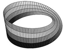
Since there are no non-trivial triple intersections, all cocycle conditions are evidently satisfied.

Accordingly by example these functions define a vector bundle.

The total space of this bundle is homeomorphic to (the interior, def. of) the Moebius strip from example .

Example

(basic complex line bundle on the 2-sphere)

Let

$$S^2 \coloneqq \left\{ (x,y,z) \;\vert\; x^2 + y^2 + z^2 = 1 \right\} \subset \mathbb{R}^3$$

be the 2-sphere with its Euclidean subspace metric topology. Let

$$\left\{ U_{i} \subset S^2 \right\}_{i \in \{+,-\}}$$

be the two complements of antipodal points

$$U_\pm \coloneqq S^2 \setminus \{(0, 0, \pm 1)\} \,.$$

Define continuous functions

$$\array{ U_+ \cap U_- &\overset{g_{\pm \mp}}{\longrightarrow}& GL(1,\mathbb{C}) \\ ( \sqrt{1-z^2} \, cos(\alpha), \sqrt{1-z^2} \, sin(\alpha), z) &\mapsto& \exp(\pm 2\pi i \alpha) } \,.$$

Since there are no non-trivial triple intersections, the only cocycle condition is

$$g_{\mp \pm} g_{\pm \mp} = g_{\pm \pm} = id$$

which is clearly satisfied.

The complex line bundle this defined is called the basic complex line bundle on the 2-sphere.

With the 2-sphere identified with the complex projective space $\mathbb{C} P^1$ (the Riemann sphere), the basic complex line bundle is the tautological line bundle (example ) on $\mathbb{C}P^1$.

Example

(clutching construction)

Generally, for $n \in \mathbb{N}$, $n \geq 1$ then the n-sphere $S^n$ may be covered by two open hemispheres intersecting in an equator of the form $S^{n-1} \times (-\epsilon, \epsilon)$. A vector bundle is then defined by specifying a single function

$$g_{+-} \;\colon\; S^{n-1} \longrightarrow GL(n,k) \,.$$

This is called the clutching construction of vector bundles over n-spheres.

Using transition functions, it is immediate how to generalize the operations of direct sum and of tensor product of vector spaces to vector bundles:

Definition

(direct sum of vector bundles)

Let $X$ be a topological space, and let $E_1 \to X$ and $E_2 \to X$ be two topological vector bundles over $X$.

Let $\{U_i \subset X\}_{i \in I}$ be an open cover with respect to which both vector bundles locally trivialize (this always exists: pick a local trivialization of either bundle and form the joint refinement of the respective open covers by intersection of their patches). Let

$$\left\{ (g_1)_{i j} \colon U_i \cap U_j \to GL(n_1) \right\} \phantom{AAA} \text{and} \phantom{AAA} \left\{ (g_2)_{i j} \colon U_i \cap U_j \longrightarrow GL(n_2) \right\}$$

be the transition functions of these two bundles with respect to this cover.

For $i, j \in I$ write

$$\array{ (g_1)_{i j} \oplus (g_2)_{i j} &\colon& U_i \cap U_j &\longrightarrow& GL(n_1 + n_2) \\ && x &\overset{\phantom{AAA}}{\mapsto}& \left( \array{ (g_1)_{i j}(x) & 0 \\ 0 & (g_2)_{i j}(x) } \right) }$$

be the pointwise direct sum of these transition functions

Then the direct sum bundle $E_1 \oplus E_2$ is the one glued from this direct sum of the transition functions (by this construction):

$$E_1 \oplus E_2 \;\coloneqq\; \left( \left( \underset{i}{\sqcup} U_i \right) \times \left( \mathbb{R}^{n_1 + n_2} \right) \right)/ \left( \left\{ (g_1)_{i j} \oplus (g_2)_{i j} \right\}_{i,j \in I} \right) \,.$$

Definition

(tensor product of vector bundles)

Let $X$ be a topological space, and let $E_1 \to X$ and $E_2 \to X$ be two topological vector bundles over $X$.

Let $\{U_i \subset X\}_{i \in I}$ be an open cover with respect to which both vector bundles locally trivialize (this always exists: pick a local trivialization of either bundle and form the joint refinement of the respective open covers by intersection of their patches). Let

$$\left\{ (g_1)_{i j} \colon U_i \cap U_j \to GL(n_1) \right\} \phantom{AAA} \text{and} \phantom{AAA} \left\{ (g_2)_{i j} \colon U_i \cap U_j \longrightarrow GL(n_2) \right\}$$

be the transition functions of these two bundles with respect to this cover.

For $i, j \in I$ write

$$\array{ (g_i)_{i j} \otimes (g_2)_{i j} &\colon& U_i \cap U_j &\longrightarrow& GL(n_1 \cdot n_2) }$$

be the pointwise tensor product of vector spaces of these transition functions

Then the tensor product bundle $E_1 \otimes E_2$ is the one glued from this tensor product of the transition functions (by this construction):

$$E_1 \otimes E_2 \;\coloneqq\; \left( \left( \underset{i}{\sqcup} U_i \right) \times \left( \mathbb{R}^{n_1 \cdot n_2} \right) \right)/ \left( \left\{ (g_1)_{i j} \otimes (g_2)_{i j} \right\}_{i,j \in I} \right) \,.$$

And so forth. For instance:

Definition

(inner product on vector bundles)

Let

1. $k$ be a topological field (such as the real numbers or complex numbers with their Euclidean metric topology ),

2. $X$ be a topological space,

3. $E \to X$ a topological vector bundle over $X$ (over $\mathbb{R}$, say).

Then an inner product on $E$ is

• a vector bundle homomorphism

  $$\langle -,-\rangle \;\colon\; E \otimes_X E \longrightarrow X \times \mathbb{R}$$

  from the tensor product of vector bundles of $E$ with itself to the trivial line bundle

such that

• for each point $x \in X$ the function

  $$\langle -,-\rangle|_x \colon E_x \otimes E_x \to \mathbb{R}$$

  is an inner product on the fiber vector space, hence a positive-definite symmetric bilinear form.

$\,$

Next we need to see how the transition functions behave under isomorphisms of vector bundles.

Definition

(coboundary between Cech cocycles )

Let $X$ be a topological space and let $c_1, c_2 \in C^1(X, \underline{GL(k)})$ be two Cech cocycles (def. ), given by

1. $\{U_i \subset X\}_{i \in I}$ and $\{U'_i \subset X\}_{i' \in I'}$ two open covers,

2. $\{g_{i j} \colon U_i \cap U_j \to GL(n,k)\}_{i,j \in I}$ and $\{g'_{i',j'} \colon U'_{i'} \cap U'_{j'} \to GL(n',k) \}_{i', j' \in I'}$ the corresponding component functions.

Then a coboundary between these two cocycles is

1. the condition that $n = n'$,

2. an open cover $\{V_\alpha \subset X\}_{\alpha \in A}\,$,

3. functions$\phi \colon A \to I$ and $\phi' \colon A \to J$ such that $\underset{\alpha \in A}{\forall}\left( \left( V_\alpha \subset U_{\phi(\alpha)} \right) \,\text{and}\, \left( V_\alpha \subset U'_{\phi'(\alpha)} \right) \right)$

4. a set $\{ \kappa_\alpha \colon V_\alpha \to GL(n,k) \}$ of continuous functions as in def.

such that

• $\underset{ \alpha, \beta \in A }{\forall} \left( \kappa_{\beta} \cdot g_{\phi(\alpha) \phi(\beta)} = g'_{\phi'(\alpha) \phi'(\beta)} \cdot \kappa_{\alpha} \,\, \text{on}\,\, V_\alpha \cap V_\beta \right)$,

  hence such that the following diagrams of linear maps commute for all $\alpha, \beta \in A$ and $x \in V_{\alpha} \cap V_\beta$:

  $$\array{ k^n &\overset{ g_{\phi(\alpha) \phi(\beta)}(x) }{\longrightarrow}& k^n \\ {}^{\mathllap{\kappa_{\alpha}(x)} }\downarrow && \downarrow^{\mathrlap{ \kappa_{\beta}(x) }} \\ k^n &\underset{ g'_{\phi'(\alpha) \phi'(\beta)}(x) }{\longrightarrow}& k^n } \,.$$

Say that two Cech cocycles are cohomologous if there exists a coboundary between them.

Example

(refinement of a Cech cocycle is a coboundary)

Let $X$ be a topological space and let $c \in C^1(X, \underline{GL(k)})$ be a Cech cocycle as in def. , with respect to some open cover $\{U_i \subset X\}_{i \in I}$, given by component functions $\{g_{i j}\}_{i,j \in I}$.

Then for $\{V_\alpha \subset X\}_{\alpha \in A}$ a refinement of the given open cover, hence an open cover such that there exists a function $\phi \colon A \to I$ with $\underset{\alpha \in A}{\forall}\left( V_\alpha \subset U_{\phi(\alpha)} \right)$, then

$$g'_{ \alpha \beta } \coloneqq g_{\phi(\alpha) \phi(\beta)} \colon V_\alpha \cap V_\beta \longrightarrow GL(n,k)$$

are the components of a Cech cocycle $c'$ which is cohomologous to $c$.

Proposition

(isomorphism of topological vector bundles induces Cech coboundary between their transition functions)

Let $X$ be a topological space, and let $c_1, c_2 \in C^1(X, \underline{GL(n,k)} )$ be two Cech cocycles as in def. .

Every isomorphism of topological vector bundles

$$f \;\colon\; E(c_1) \overset{\simeq}{\longrightarrow} E(c_2)$$

between the vector bundles glued from these cocycles according to def. induces a coboundary between the two cocycles,

$$c_1 \sim c_2 \,,$$

according to def. .

Proof

By example we may assume without restriction that the two Cech cocycles are defined with respect to the same open cover $\{U_i \subset X\}_{i \in I}$ (for if they are not, then by example both are cohomologous to cocycles on a joint refinement of the original covers and we may argue with these).

Accordingly, by example the two bundles $E(c_1)$ and $E(c_2)$ both have local trivializations of the form

$$\{ U_i \times k^n \underoverset{\simeq}{\phi^1_i}{\longrightarrow} E(c_1)\vert_{U_i}\}$$

and

$$\{ U_i \times k^n \underoverset{\simeq}{\phi^2_i}{\longrightarrow} E(c_2)\vert_{U_i}\}$$

over this cover. Consider then for $i \in I$ the function

$$f_i \coloneqq (\phi_i^2)^{-1}\circ f\vert_{U_i} \circ \phi^1_i \,,$$

hence the unique function making the following diagram commute:

$$\array{ U_i \times k^n &\underoverset{\simeq}{\phi^1_i}{\longrightarrow}& E(c_1)\vert_{U_i} \\ {}^{\mathllap{f_i}}\downarrow && \downarrow^{\mathrlap{ f\vert_{U_i} }} \\ U_i \times k^n &\underoverset{\phi^2_i}{\simeq}{\longrightarrow}& E(c_2)\vert_{U_i} } \,.$$

This induces for all $i,j \in I$ the following composite commuting diagram

$$\array{ (U_i \cap U_j) \times k^n &\underoverset{\simeq}{\phi^1_i}{\longrightarrow}& E(c_1)\vert_{U_i \cap U_j} & \underoverset{\simeq}{(\phi^1_j)^{-1}}{\longrightarrow} & (U_i \cap U_j) \times k^n \\ {}^{\mathllap{f_i}}\downarrow && \downarrow^{\mathrlap{ f\vert_{U_i \cap U_j} }} && \downarrow^{\mathrlap{ f_j }} \\ (U_i \cap U_j) \times k^n &\underoverset{\phi^2_i}{\simeq}{\longrightarrow}& E(c_2)\vert_{U_1 \cap U_2} &\underoverset{(\phi^2_j)^{-1}}{\simeq}{\longrightarrow}& (U_i \cap U_j) \times k^n } \,.$$

By construction, the two horizonal composites of this diagram are pointwise given by the components $g^1_{i j}$ and $g^2_{i j}$of the cocycles $c_1$ and $c_2$, respectively. Hence the commutativity of this diagram is equivalently the commutativity of these diagrams:

$$\array{ k^n &\overset{ g^1_{i j}(x) }{\longrightarrow}& k^n \\ {}^{\mathllap{ f_i(x) } }\downarrow && \downarrow^{\mathrlap{ f_j(x) }} \\ k^n &\underset{ g^2_{ i j }(x) }{\longrightarrow}& k^n } \,.$$

for all $i,j \in I$ and $x \in U_i \cap U_j$. By def. this exhibits the required coboundary.

Definition

(Cech cohomology)

Let $X$ be a topological space. The relation $\sim$ on Cech cocycles of being cohomologous (def. ) is an equivalence relation on the set $C^1( X, \underline{GL(k)} )$ of Cech cocycles (def. ).

Write

$$H^1(X, \underline{GL(k)} ) \;\coloneqq\; C^1(X, \underline{GL(k)} )/\sim$$

for the resulting set of equivalence classes. This is called the Cech cohomology of $X$ in degree 1 with coefficients in $\underline{GL(k)}$.

Proposition

(Cech cohomology computes isomorphism classes of topological vector bundle)

Let $X$ be a topological space.

The construction of gluing a topological vector bundle from a Cech cocycle (example ) constitutes a bijection between the degree-1 Cech cohomology of $X$ with coefficients in $GL(n,k)$ (def. ) and the set of isomorphism classes of topological vector bundles on $X$ (def. , remark ):

$$\array{ H^1(X,\underline{GL(k)}) &\overset{\phantom{AA}\simeq \phantom{AA}}{\longrightarrow}& Vect(X)_{/\sim} \\ c &\overset{\phantom{AAA}}{\mapsto}& E(c) } \,.$$

Proof

First we need to see that the function is well defined, hence that if cocycles $c_1, c_2 \in C^1(X,\underline{GL(k)})$ are related by a coboundary, $c_1 \sim c_2$ (def. ), then the vector bundles $E(c_1)$ and $E(c_2)$ are related by an isomorphism.

Let $\{V_\alpha \subset X\}_{\alpha \in A}$ be the open cover with respect to which the coboundary $\{\kappa_\alpha \colon V_\alpha \to GL(n,k)\}_{\alpha}$ is defined, with refining functions $\phi \colon A \to I$ and $\phi' \colon A \to I'$. Let $\left\{ \mathbb{R}^n \underoverset{\simeq}{\psi_{\phi(\alpha)}\vert_{V_\alpha} }{\to} E(c_1)\vert_{V_\alpha} \right\}_{\alpha \in A}$ and $\left\{ V_\alpha \times k^n \underoverset{\simeq}{\psi'_{\phi'(\alpha)}\vert_{V_\alpha} }{\to} E(c_2)\vert_{V_\alpha} \right\}_{\alpha \in A}$ be the corresponding restrictions of the canonical local trivilizations of the two glued bundles.

For $\alpha \in A$ define

$$f_\alpha \coloneqq \psi'_{\phi'(\alpha)}\vert_{V_\alpha} \circ \kappa_\alpha \circ (\psi_{\phi(\alpha)}\vert_{V_\alpha} )^{-1} \phantom{AAAA} \text{hence:} \phantom{AAA} \array{ V_\alpha \times k^n &\overset{ \psi_{\phi(\alpha)}\vert_{V_\alpha} }{\longrightarrow}& E(c_1)\vert_{V_\alpha} \\ {}^{\mathllap{\kappa_\alpha}}\downarrow && \downarrow^{\mathrlap{f_\alpha}} \\ V_\alpha \times k^n &\overset{ (\psi'_{\phi'(\alpha)}\vert_{V_\alpha})^{-1} }{\longleftarrow}& E(c_1)\vert_{V_\alpha} } \,.$$

Observe that for $\alpha, \beta \in A$ and $x \in V_\alpha \cap V_\beta$ the coboundary condition implies that

$$f_\alpha\vert_{V_\alpha \cap V_\beta} \;=\; f_\beta\vert_{V_\alpha \cap V_\beta}$$

because in the diagram

$$\array{ k^n &\overset{ g_{\phi(\alpha) \phi(\beta) }(x) }{\longrightarrow}& k^n \\ {}^{\mathllap{\kappa_\alpha(x)}}\downarrow && \downarrow^{\mathrlap{\kappa_{\beta}(x)}} \\ k^n &\underset{g'_{\phi'(\alpha) \phi'(\beta)}(x) }{\longrightarrow}& k^n } \phantom{AAAAA} = \phantom{AAAAA} \array{ k^n &\overset{ \psi_{\phi(\alpha)}(x) }{\longrightarrow}& E(c_1)_x &\overset{ (\psi_{\phi(\beta)})^{-1}(x) }{\longrightarrow}& k^n \\ {}^{\mathllap{\kappa_\alpha(x)}}\downarrow && \downarrow^{\mathrlap{\exists !} } && \downarrow^{\mathrlap{\beta_\alpha(x)}} \\ k^n &\overset{ \psi'_{\phi'(\alpha)}(x) }{\longrightarrow}& E(c_2)_x &\overset{ (\psi'_{\phi'(\beta)})^{-1}(x) }{\longrightarrow}& k^n }$$

the vertical morphism in the middle on the right is unique, by the fact that all other morphisms in the diagram on the right are invertible.

Therefore by example there is a unique vector bundle homomorphism

$$f\;\colon\; E(c_1) \to E(c_2)$$

given for all $\alpha \in A$ by $f\vert_{V_\alpha} = f_\alpha$. Similarly there is a unique vector bundle homomorphism

$$f^{-1}\;\colon\; E(c_2) \to E(c_1)$$

given for all $\alpha \in A$ by $f^{-1}\vert_{V_\alpha} = f^{-1}_\alpha$. Hence this is the required vector bundle isomorphism.

Finally to see that the function from Cech cohomology classes to isomorphism classes of vector bundles thus defined is a bijection:

By prop. the function is surjective, and by prop. it is injective.

$\,$

Properties

We discuss some basic general properties of topological vector bundles.

Lemma

(homomorphism of vector bundles is isomorphism as soon as it is a fiberwise isomorphism)

Let $[E_1 \to X]$ and $[E_2 \to X]$ be two topological vector bundles (def. ).

If a homomorphism of vector bundles $f \colon E_1 \longrightarrow E_2$ restricts on the fiber over each point to a linear isomorphism

$$f\vert_x \;\colon\; (E_1)_x \overset{\simeq}{\longrightarrow} (E_2)_x$$

then $f$ is already an isomorphism of vector bundles.

Proof

It is clear that $f$ has an inverse function

of underlying sets $f^{-1} \colon E_2 \to E_1$ which is a function over $X$: Over each $x \in X$ it it the linear inverse $(f\vert_x)^{-1} \colon (E_2)_x \to (E_1)_x$.

What we need to show is that this is a continuous function.

By remark we find an open cover $\{U_i \subset X\}_{i \in I}$ over which both bundles have a local trivialization.

$$\left\{ U_i \underoverset{\simeq}{\phi^1_i}{\to} (E_1)\vert_{U_i}\right\}_{i \in I} \phantom{AA} \text{and} \phantom{AA} \left\{ U_i \underoverset{\simeq}{\phi^2_i}{\to} (E_2)\vert_{U_i} \right\}_{i \in I} \,.$$

Restricted to any patch $i \in I$ of this cover, the homomorphism $f|_{U_i}$ induces a homomorphism of trivial vector bundles

$$f_i \coloneqq \phi^2_j^{-1} \circ f \circ \phi^1_i \phantom{AAAAAA} \array{ U_i \times k^n &\underoverset{\simeq}{\phi^1_i}{\longrightarrow}& (E_1)\vert|_{U_i} \\ {}^{f_i}\downarrow && \downarrow^{\mathrlap{f\vert_{U_i}}} \\ U_i \times k^n &\underoverset{\phi^2_i}{\simeq}{\longrightarrow}& (E_2)\vert_{U_j} } \,.$$

Also the $f_i$ are fiberwise invertible, hence are continuous bijections. We claim that these are homeomorphisms, hence that their inverse functions $(f_i)^{-1}$ are also continuous.

To this end we re-write the $f_i$ a little. First observe that by the universal property of the product topological space and since they fix the base space $U_i$, the $f_i$ are equivalently given by a continuous function

$$h_i \;\colon\; U_i \times k^n \longrightarrow k^n$$

as

$$f_i(x,v) = (x, h_i(x,v)) \,.$$

Moreover since $k^n$ is locally compact (as every metric space), the mapping space adjunction says (by prop. ) that there is a continuous function

$$\tilde h_i \;\colon\; U_i \longrightarrow Maps(k^n, k^n)$$

(with $Maps(k^n,k^n)$ the set of continuous functions $k^n \to k^n$ equipped with the compact-open topology) which factors $h_i$ via the evaluation map as

$$h_i \;\colon\; U_i \times k^n \overset{\tilde h_i \times id_{k^n}}{\longrightarrow} Maps(k^n, k^n) \times k^n \overset{ev}{\longrightarrow} k^n \,.$$

By assumption of fiberwise linearity the functions $\tilde h_i$ in fact take values in the general linear group

$$GL(n,k) \subset Maps(k^n, k^n)$$

and this inclusion is a homeomorphism onto its image (by this prop.).

Since passing to inverse matrices

$$(-)^{-1} \;\colon\; GL(n,k) \longrightarrow GL(n,k)$$

is a rational function on its domain $GL(n,k) \subset Mat_{n \times n}(k) \simeq k^{(n^2)}$ inside Euclidean space and since rational functions are continuous on their domain of definition, it follows that the inverse of $f_i$

$$(f_i)^{-1} \;\colon\; U_i \times k^n \overset{(id , \tilde h_i ) }{\longrightarrow} U_i \times k^n \times GL(n,k) \overset{ id \times (-)^{-1} }{\longrightarrow} U_i \times k^n \times GL(n,k) \overset{id \times ev}{\longrightarrow} U_i \times k^n$$

is a continuous function.

To conclude that also $f^{-1}$ is a continuous function we make use prop. to find an isomorphism between $E_2$ and a quotient topological space of the form

$$E_2 \simeq \left(\underset{i \in I}{\sqcup} (U_i \times k^n) \right) / \left( \left\{ g_{i j}\right\}_{i,j\in I} \right) \,.$$

Hence $f^{-1}$ is equivalently a function on this quotient space, and we need to show that as such it is continuous.

By the universal property of the disjoint union space (the coproduct in Top) the set of continuous functions

$$\{ U_i \times k^n \overset{f_i^{-1}}{\to} U_i \times k^n \overset{\phi^1_i}{\to} E_1 \}_{i \in I}$$

corresponds to a single continuous function

$$(\phi^1_i \circ f_i^{-1})_{i \in I} \;\colon\; \underset{i \in I}{\sqcup} U_i \times k^n \longrightarrow E_1 \,.$$

These functions respect the equivalence relation, since for each $x \in U_i \cap U_j$ we have

$$(\phi^1_i \circ f_i^{-1})((x,i),v) = (\phi^1_j \circ f_j^{-1})( (x,j), g_{i j}(x)(v) ) \phantom{AAAA} \text{since:} \phantom{AAAA} \array{ && E_1 \\ & {}^{\mathllap{\phi^1_i \circ f_i^{-1}}}\nearrow & \uparrow^{\mathrlap{f^{-1}}} & \nwarrow^{\mathrlap{ \phi^1_j \circ f_j^{-1} }} \\ U_i \times k^n &\underset{\phi^2_i}{\longrightarrow}& (E_2)\vert_{U_i \cap U_i} &\underset{(\phi^2_j)^{-1}}{\longrightarrow}& U_i \times k^n } \,.$$

Therefore by the universal property of the quotient topological space $E_2$, these functions extend to a unique continuous function $E_2 \to E_1$ such that the following diagram commutes:

$$\array{ \underset{i \in i}{\sqcup} U_i \times k^n &\overset{( \phi^1_i \circ f_i^{-1} )_{i \in I}}{\longrightarrow}& E_1 \\ \downarrow & \nearrow_{\mathrlap{\exists !}} \\ E_2 } \,.$$

This unique function is clearly $f^{-1}$ (by pointwise inspection) and therefore $f^{-1}$ is continuous.

Example

(fiberwise linearly independent sections trivialize a vector bundle)

If a topological vector bundle $E \to X$ of rank $n$ admits $n$ sections (example )

$$\{\sigma_k \;\colon\; X \longrightarrow E\}_{k \in \{1, \cdots, n\}}$$

that are linearly independent at each point $x \in X$, then $E$ is trivializable (example ). In fact, with the sections regarded as vector bundle homomorphisms out of the trivial vector bundle of rank $n$ (according to example ), these sections are the trivialization

$$(\sigma_1, \cdots, \sigma_n) \;\colon\; (X \times k^n) \overset{\simeq}{\longrightarrow} E \,.$$

This is because their linear independence at each point means precisely that this morphism of vector bundles is a fiber-wise linear isomorphism and therefore an isomorphism of vector bundles by lemma .

$\,$

(…)

$\,$

Manifolds

A topological manifold is a topological space which is locally homeomorphic to a Euclidean space (def. below), but which may globally look very different. These are the kinds of topological spaces that are really meant when people advertise topology as “rubber-sheet geometry”.

If the gluing functions which relate the Euclidean local charts of topological manifolds to each other are differentiable functions, for a fixed degree of differentiability, then one speaks of differentiable manifolds (def below) or of smooth manifolds if the gluing functions are arbitrarily differentiable.

Accordingly, a differentiable manifold is a space to which the tools of infinitesimal analysis may be applied locally. In particular we may ask whether a continuous function between differentiable manifolds is differentiable by computing its derivatives pointwise in any of the Euclidean coordinate charts. This way differential and smooth manifolds are the basis for what is called differential geometry. (They are the analogs in differential geometry of what schemes are in algebraic geometry.)

Basic examples of smooth manifolds are the n-spheres (example below), the projective spaces (example below). and the general linear group (example ) below.

$\,$

The definition of topological manifolds (def. below) involves two clauses: The conceptual condition is that a manifold is locally Euclidean topological space (def. below). On top of this one demands as a technical regularity condition paracompact Hausdorffness, which serves to ensure that manifolds behave well. Therefore we first consider locally Euclidean spaces in themselves.

Definition

(locally Euclidean topological space)

A topological space $X$ is locally Euclidean if every point $x \in X$ has an open neighbourhood $U_x \supset \{x\}$ which, as a subspace (example ), is homeomorphic (def. ) to the Euclidean space $\mathbb{R}^n$ (example ) with its metric topology (def. ):

$$\mathbb{R}^n \overset{\phantom{AA} \simeq \phantom{AA}}{\longrightarrow} U_x \subset X \,.$$

The “local” topological properties of Euclidean space are inherited by locally Euclidean spaces:

Proposition

(locally Euclidean spaces are $T_1$-separated, sober, locally compact, locally connected and locally path-connected topological spaces)

Let $X$ be a locally Euclidean space (def. ). Then

1. $X$ satisfies the $T_1$ separation axiom (def. );

2. $X$ is sober (def. );

3. $X$ is locally compact in the weak sense of def. .

4. $X$ is locally connected (def. ),

5. $X$ is locally path-connected (def. ).

Proof

Regarding the first statement:

Let $x \neq y$ be two distinct points in the locally Euclidean space. We need to show that there is an open neighbourhood $U_x$ around $x$ that does not contain $y$.

By definition, there is a Euclidean open neighbourhood $\mathbb{R}^n \underoverset{\simeq}{\phi}{\to} U_x \subset X$ around $x$. If $U_x$ does not contain $y$, then it already is an open neighbourhood as required. If $U_x$ does contain $y$, then $\phi^{-1}(x) \neq \phi^{-1}(y)$ are equivalently two distinct points in $\mathbb{R}^n$. But Euclidean space, as every metric space, is $T_1$ (example , prop. ), and hence we may find an open neighbourhood $V_{\phi^{-1}(x)} \subset \mathbb{R}^n$ not containing $\phi^{-1}(y)$. By the nature of the subspace topology, $\phi(V_{\phi^{-1}(x)}) \subset X$ is an open neighbourhood as required.

Regarding the second statement:

We need to show that the map

$$Cl(\{-\}) \;\colon\; X \to IrrClSub(X)$$

that sends points to the topological closure of their singleton sets is a bijection with the set of irreducible closed subsets. By the first statement above the map is injective (via lemma ). Hence it remains to see that every irreducible closed subset is the topological closure of a singleton. We will show something stronger: every irreducible closed subset is a singleton.

Let $P \subset X$ be an open proper subset such that if there are two open subsets $U_1, U_2 \subset X$ with $U_1 \cap U_2 \subset P$ then $U_1 \subset P$ or $U_2 \subset P$. By prop ) we need to show that there exists a point $x \in X$ such that $P = X \setminus \{x\}$ it its complement.

Now since $P \subset X$ is a proper subset, and since the locally Euclidean space $X$ is covered by Euclidean neighbourhoods, there exists a Euclidean neighbourhood $\mathbb{R}^n \underoverset{\simeq}{\phi}{\to} U \subset X$ such that $P \cap U \subset U$ is a proper subset. In fact this still satisfies the condition that for $U_1, U_2 \underset{\text{open}}{\subset} U$ then $U_1 \cap U_2 \subset P \cap U$ implies $U_1 \subset P \cap U$ or $U_2 \subset P \cap U$. Accordingly, by prop. , it follows that $\mathbb{R}^n \setminus \phi^{-1}(P \cap U)$ is an irreducible closed subset of Euclidean space. Sine metric spaces are sober topological space as well as $T_1$-separated (example , prop. ), this means that there exists $x \in \mathbb{R}^n$ such that $\phi^{-1}(P \cap U) = \mathbb{R}^n \setminus \{x\}$.

In conclusion this means that the restriction of an irreducible closed subset in $X$ to any Euclidean chart is either empty or a singleton set. This means that the irreducible closed subset must be a disjoint union of singletons that are separated by Euclidean neighbourhoods. But by irreducibiliy, this union has to consist of just one point.

Regarding the third statement:

Let $x \in X$ be a point and let $U_x \supset \{x\}$ be an open neighbourhood. We need to find a compact neighbourhood $K_x \subset U_x$.

By assumption there exists a Euclidean open neighbourhood $\mathbb{R}^n \underoverset{\simeq}{\phi}{\to} V_x \subset X$. By definition of the subspace topology the intersection $U_x \cap V_x$ is still open as a subspace of $V_x$ and hence $\phi^{-1}(U_x \cap V_x)$ is an open neighbourhood of $\phi^{-1}(x) \in \mathbb{R}^n$.

Since Euclidean spaces are locally compact (example ), there exists a compact neighbourhood $K_{\phi^{-1}(x)} \subset \mathbb{R}^n$ (for instance a sufficiently small closed ball around $x$, which is compact by the Heine-Borel theorem, prop. ). Now since continuous images of compact spaces are compact prop. , it follows that also $\phi(K) \subset X$ is a compact neighbourhood.

Regarding the last two statements:

We need to show that for every point $x \in X$ and every [neighbourhood there exists a neighbourhood which is and a neighbourhood which is .]

By local Euclideanness there exists a chart $\mathbb{R}^n \underoverset{\simeq}{\phi}{\to} V_x \subset X$. Since Euclidean space is locally connected and locally path-connected (def. ), there is a connected and a path-connected neighbourhood of the pre-image $\phi^{-1}(x)$ contained in the pre-image $\phi^{-1}( U_x \cap V_x )$. Since continuous images of connected spaces are connected (prop. ), and since continuous images of path-connected spaces are path-connected (prop. ), the images of these neighbourhoods under $\phi$ are neighbourhoods of $x$ as required.

It follows immediately from prop. via prop. that:

Proposition

(connected locally Euclidean spaces are path-connected)

For a locally Euclidean space $(X,\tau)$ (def. ) the connected components (def. ) coincide with the path-connected components (def. ).

But the “global” topological properties of Euclidean space are not generally inherited by locally Euclidean spaces. This sounds obvious, but notice that also Hausdorff-ness is a “global property”:

Remark

(locally Euclidean spaces are not necessarily $T_2$)

It might superficially seem that every locally Euclidean space (def. ) is necessarily a Hausdorff topological space, since Euclidean space, like any metric space, is Hausdorff, and since by definition the neighbourhood of every point in a locally Euclidean spaces looks like Euclidean space.

But this is not so, see the counter-example below, Hausdorffness is a “non-local condition”, as opposed to the $T_0$ and $T_1$ separation axioms.

Nonexample

(non-Hausdorff locally Euclidean spaces)

An example of a locally Euclidean space (def. ) which is a non-Hausdorff topological space, is the line with two origins (example ).

Therefore we will explicitly impose Hausdorffness on top of local Euclidean-ness. This implies the equivalence of following further regularity properties:

Proposition

(equivalence of regularity conditions for locally Euclidean Hausdorff spaces)

Let $X$ be a locally Euclidean space (def. ) which is Hausdorff (def. ).

Then the following are equivalent:

1. $X$ is sigma-compact (def. ).

2. $X$ is second-countable (def. ).

3. $X$ is paracompact (def. ) and has a countable set of connected components (def. ).

Proof

First, observe that $X$ is locally compact in the strong sense of def. : By prop. every locally Euclidean space is locally compact in the weak sense that every neighbourhood contains a compact neighbourhood, but since $X$ is assumed to be Hausdorff, this implies the stronger statement by prop. .

1) $\Rightarrow$ 2)

Let $X$ be sigma-compact. We show that then $X$ is second-countable:

By sigma-compactness there exists a countable set $\{K_i \subset X\}_{i \in I}$ of compact subspaces. By $X$ being locally Euclidean, each $K_i$ admits an open cover by restrictions of Euclidean spaces. By their compactness, each $K_i$ has a subcover

$$\{ \mathbb{R}^{n_{j}} \overset{\phi_{i,j}}{\to} X \}_{j \in J_i}$$

with $J_i$ a finite set. Since countable unions of countable sets are countable, we have obtained a countable cover of $X$ by Euclidean spaces $\{ \mathbb{R}^n \overset{\phi_{i,j}}{\to} X\}_{i \in I, j \in J_i}$. Now Euclidean space itself is second countable (by example ), hence admits a countable set $\beta_{\mathbb{R}^n}$ of base open sets. As a result the union $\underset{{i \in I} \atop {j \in J_i}}{\cup} \phi_{i,j}(\beta_{\mathbb{R}^n})$ is a base of opens for $X$. But this is a countable union of countable sets, and since countable unions of countable sets are countable we have obtained a countable base for the topology of $X$. This means that $X$ is second-countable.

1) $\Rightarrow$ 3)

Let $X$ be sigma-compact. We show that then $X$ is paracompact with a countable set of connected components:

Since locally compact and sigma-compact spaces are paracompact (prop. ), it follows that $X$ is paracompact. By local connectivity (prop. ) $X$ is the disjoint union space of its connected components (def. , lemma ). Since, by the previous statement, $X$ is also second-countable it cannot have an uncountable set of connected components. (Because there must be at least one base open contained in every connected component.)

2)$\Rightarrow$ 1) Let $X$ be second-countable, we need to show that it is sigma-compact.

This follows since locally compact and second-countable spaces are sigma-compact (lemma ).

3) $\Rightarrow$ 1)

Now let $X$ be paracompact with countably many connected components. We show that $X$ is sigma-compact.

By local compactness, there exists an open cover $\{U_i \subset X\}_{i \in I}$ such that the topological closures $\{K_i \coloneqq Cl(U_i) \subset X\}_{i \in I}$ constitute a cover by compact subspaces. By paracompactness there is a locally finite refinement of this cover. Since paracompact Hausdorff spaces are normal (prop. ), the shrinking lemma applies (lemma ) to this refinement and yields a locally finite open cover

$$\mathcal{V} \coloneqq \{V_j \subset X \}_{j \in J}$$

as well as a locally finite cover $\{Cl(V_j) \subset X\}_{j \in J}$ by closed subsets. Since this is a refinement of the original cover, all the $Cl(V_j)$ are contained in one of the compact subspaces $K_i$. Since subsets are closed in a closed subspace precisely if they are closed in the ambient space (lemma ), the $Cl(V_j)$ are also closed as subsets of the $K_i$. Since closed subsets of compact spaces are compact (lemma ) it follows that the $Cl(V_j)$ are themselves compact and hence form a locally finite cover by compact subspaces.

Now fix any $j_0 \in J$.

We claim that for every $j \in J$ there is a finite sequence of indices $(j_0, j_1, \cdots, j_n, j_{n} = j)$ with the property that $V_{j_k} \cap V_{j_{k+1}} \neq \emptyset$ for all $k \in \{0, \cdots, n\}$.

To see this, first observe that it is sufficient to show sigma-compactness for the case that $X$ is connected. From this the general statement follows since countable unions of countable sets are countable. Hence assume that $X$ is connected. It follows from prop. that $X$ is path-connected.

Hence for any $x \in V_{j_0}$ and $y \in V_{j}$ there is a path $\gamma \colon [0,1] \to X$ (def. ) connecting $x$ with $y$. Since the closed interval is compact (example ) and since continuous images of compact spaces are compact (prop. ), it follows that there is a finite subset of the $V_i$ that covers the image of this path. This proves the claim.

It follows that there is a function

$$f \;\colon\; \mathcal{V} \longrightarrow \mathbb{N}$$

which sends each $V_j$ to the minimum natural number $n$ as above.

We claim now that for all $n \in \mathbb{N}$ the preimage of $\{0,1, \cdots, n\}$ under this function is a finite set. Since countable unions of countable sets are countable this means that $f$ serves as a countable enumeration of the set $J$ and hence implies that $\{ Cl(V_j) \subset X\}_{j \in J}$ is a countable cover of $X$ by compact subspaces, hence that $X$ is sigma-compact.

We prove this last claim by induction. It is true for $n = 0$ by construction, since $f^{-1}(\{0\}) = V_{j_0}$. Assume it is true for some $n \in \mathbb{N}$, hence that $f^{-1}(\{0,1, \cdots, n\})$ is a finite set. Since finite unions of compact subspaces are again compact (example ) it follows that

$$K_n \coloneqq \underset{V \in f^{-1}(\{0,\cdots, n\})}{\cup} Cl(V)$$

is compact. By local finiteness of the $\{Cl(V_j)\}_{j \in J}$, every point $x \in K_n$ has an open neighbourhood $W_x$ that intersects only a finite set of the $Cl(V_j)$. By compactness of $K_n$, the cover $\{W_x \cap K_nfGi \subset K_n\}_{x \in K_n}$ has a finite subcover. In conclusion this implies that only a finite number of the $V_j$ intersect $K_n$.

Now by definition $f^{-1}(\{0,1,\cdots, n+1\})$ is a subset of those $V_j$ which intersect $K_n$, and hence itself finite.

This finally gives a good idea of what the definition of topological manifolds should be:

Definition

(topological manifold)

A topological manifold is a topological space which is

1. locally Euclidean (def. ),

2. paracompact Hausdorff (def. , def. ).

If the Euclidean neighbourhoods $\mathbb{R}^n \overset{\simeq}{\to} U_x \subset X$ of the points $x \in X$ are all of dimension $n$ for some $n \in \mathbb{N}$, then the topological manifold is said to be of dimension $n$, too. Sometimes one also speaks of an “$n$-fold” in this case.

Remark

(varying terminology regarding “topological manifold”)

Often a topological manifold (def. ) is required to be second-countable (def. ) or sigma-compact (def. ). But by prop. both conditions are implied by def. as soon as there is a countable set of connected components. Manifolds with uncountably many connected components are rarely considered in practice. The restriction to countably many connected components is strictly necessary for several important theorems (beyond the scope of our discussion here) such as:

1. the Whitney embedding theorem;

2. the embedding of smooth manifolds into formal duals of R-algebras.

Besides the trivial case of Euclidean spaces themselves, we discuss here three main classes of examples of manifolds:

1. n-spheres$S^n$ (example below)

2. projective spaces$k P^n$ (example below)

3. general linear groups$GL(n,k)$ (example ) below.

Since all these examples are not just topological manifolds but naturally carry also the structure of differentiable manifolds, we first consider this richer definition before turning to the examples:

Definition

(local chart, atlas and gluing function)

Given an $n$-dimensional topological manifold $X$ (def. ), then

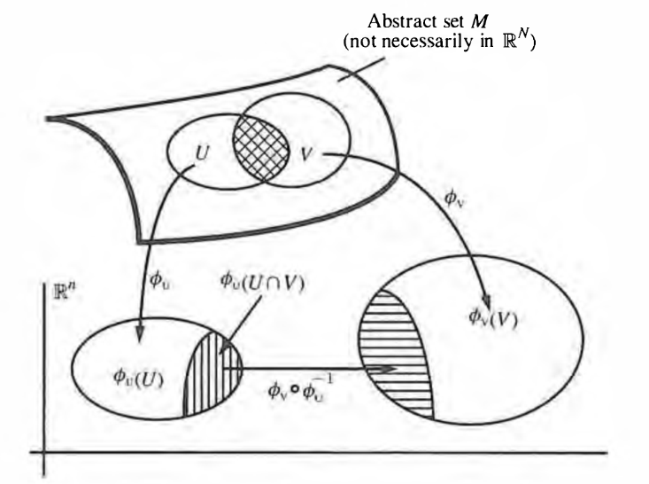
1. An open subset $U \subset X$ and a homeomorphism $\phi \colon \mathbb{R}^n \overset{\phantom{A}\simeq\phantom{A}}{\to} U$ from the $n$-dimensional Euclidean space is also called a local coordinate chart of $X$.

2. An open cover of $X$ by local charts $\left\{ \mathbb{R}^n \underoverset{\simeq}{\phi_i}{\to} U \subset X \right\}_{i \in I}$ is called an atlas of the topological manifold.

3. Given such an atlas then for each $i,j \in I$ the induced homeomorphism

   $$\mathbb{R}^n \supset \phantom{AA} \phi_i^{-1}(U_i \cap U_j) \overset{\phantom{A}\phi_i\phantom{A}}{\longrightarrow} U_i \cap U_j \overset{\phantom{A}\phi_j^{-1}\phantom{A}}{\longrightarrow} \phi_j^{-1}(U_i \cap U_j) \phantom{AA} \subset \mathbb{R}^n$$

   is called the coordinate transformation or gluing function from chart $i$ to chart $j$.

graphics grabbed from Frankel

Next we consider the case that the gluing functions of a topological manifold are differentiable functions in which case one speaks of a differentiable manifold (def. below). For convenience we first recall the definition of differentiable functions between Euclidean spaces:

Definition

(differentiable functions between Euclidean spaces)

Let $n \in \mathbb{N}$ and let $U \subset \mathbb{R}^n$ be an open subset of Euclidean space (example ).

Then a function $f \;\colon\; U \longrightarrow \mathbb{R}$ is called differentiable at $x\in U$ if there exists a linear map $d f_x : \mathbb{R}^n \to \mathbb{R}$ such that the following limit exists and vanishes as $h$ approaches zero “from all directions at once”:

$$\lim_{h\to 0} \frac{f(x+h)-f(x) - d f_x(h)}{\Vert h\Vert} = 0.$$

This means that for all $\epsilon \in (0,\infty)$ there exists an open neighbourhood $V_x\subseteq U$ of $x$ such that whenever $x+h\in V$ we have $\frac{f(x+h)-f(x) - d f_x(h)}{\Vert h\Vert} \lt \epsilon$.

We say that $f$ is differentiable on a subset $S$ of $U$ if $f$ is differentiable at every $x\in S$, and we say that $f$ is differentiable if $f$ is differentiable on all of $U$. We say that $f$ is continuously differentiable if it is differentiable and $d f$ is a continuous function.

The function $d f_x$ is called the derivative or differential of $f$ at $x$.

More generally, let $n_1, n_2 \in \mathbb{N}$ and let $U\subseteq \mathbb{R}^{n_1}$ be an open subset.

Then a function $f \;\colon\; U \longrightarrow \mathbb{R}^{n_2}$ is differentiable if for all $i \in \{1, \cdots, n_2\}$ the component function

$$f_i \;\colon\; U \overset{f}{\longrightarrow} \mathbb{R}^{n_2} \overset{pr_i}{\longrightarrow} \mathbb{R}$$

is differentiable in the previous sense

In this case, the derivatives $d f_i \colon \mathbb{R}^n \to \mathbb{R}$ of the $f_i$ assemble into a linear map of the form

$$d f_x \;\colon\; \mathbb{R}^{n_1} \to \mathbb{R}^{n_2} \,.$$

If the derivative exists at each $x \in U$, then it defines itself a function

$$d f \;\colon\; U \longrightarrow Hom_{\mathbb{R}}(\mathbb{R}^{n_1} , \mathbb{R}^{n_2}) \simeq \mathbb{R}^{n_1 \cdot n_2}$$

to the space of linear maps from $\mathbb{R}^{n_1}$ to $\mathbb{R}^{n_2}$, which is canonically itself a Euclidean space. We say that $f$ is twice continuously differentiable if $d f$ is continuously differentiable.

Generally then, for $k \in \mathbb{N}$ the function $f$ is called $k$-fold continuously differentiable or of class $C^k$ if for all $j \leq k$ the $j$-fold differential $d^j f$ exists and is a continuous function.

Finally, if $f$ is $k$-fold continuously differentiable for all $k \in \mathbb{N}$ then it is called a smooth function or of class $C^\infty$.

Of the various properties satisfied by differentiation, the following plays a special role in the theory of differentiable manifolds (notably in the discussion of their tangent bundles, def. below):

Proposition

(chain rule for differentiable functions between Euclidean spaces)

Let $n_1, n_2, n_3 \in \mathbb{N}$ and let

$$\mathbb{R}^{n_1} \overset{f}{\longrightarrow} \mathbb{R}^{n_2} \overset{g}{\longrightarrow} \mathbb{R}^{n_3}$$

be two differentiable functions (def. ). Then the derivative of their composite is the composite of their derivatives:

$$d(g \circ f)_x = d g_{f(x)} \circ d f_x \,.$$

Definition

(differentiable manifold and smooth manifold)

For $p \in \mathbb{N} \cup \{\infty\}$ then a $p$-fold differentiable manifold or $C^p$-manifold for short is

1. a topological manifold $X$ (def. );

2. an atlas $\{\mathbb{R}^n \overset{\phi_i}{\to} X\}$ (def. ) all whose gluing functions are $p$ times continuously differentiable.

A $p$-fold differentiable function between $p$-fold differentiable manifolds

$$\left(X,\, \{\mathbb{R}^{n} \overset{\phi_i}{\to} U_i \subset X\}_{i \in I} \right) \overset{\phantom{AA}f\phantom{AA}}{\longrightarrow} \left(Y,\, \{\mathbb{R}^{n'} \overset{\psi_j}{\to} V_j \subset Y\}_{j \in J} \right)$$

is

• a continuous function $f \colon X \to Y$

such that

• for all $i \in I$ and $j \in J$ then

  $$\mathbb{R}^n \supset \phantom{AA} (f\circ \phi_i)^{-1}(V_j) \overset{\phi_i}{\longrightarrow} f^{-1}(V_j) \overset{f}{\longrightarrow} V_j \overset{\psi_j^{-1}}{\longrightarrow} \mathbb{R}^{n'}$$

  is a $p$-fold differentiable function between open subsets of Euclidean space.

(Notice that this in in general a non-trivial condition even if $X = Y$ and $f$ is the identity function. In this case the above exhibits a passage to a different, but equivalent, differentiable atlas.)

If a manifold is $C^p$ differentiable for all $p$, then it is called a smooth manifold. Accordingly a continuous function between differentiable manifolds which is $p$-fold differentiable for all $p$ is called a smooth function,

Remark

(category Diff of differentiable manifolds)

In analogy to remark there is a category called Diff${}_p$ (or similar) whose objects are $C^p$-differentiable manifolds and whose morphisms are $C^p$-differentiable functions, for given $p \in \mathbb{N} \cup \{\infty\}$.

The analog of the concept of homeomorphism (def. ) is now this:

Definition

(diffeomorphism)

Given smooth manifolds $X$ and $Y$ (def. ), then a smooth function

$$f \;\colon\; X \longrightarrow Y$$

is called a diffeomorphism, if there is an inverse function

$$X \longleftarrow Y \;\colon\; g$$

which is also a smooth function (hence if $f$ is an isomorphism in the category Diff${}_\infty$ from remark ).

Remark

(basic properties of diffeomorphisms)

Let $X,Y$ be differentiable manifolds (def. ). Let

$$f \colon X \longrightarrow Y$$

be a diffeomorphisms (def. ) with inverse differentiable function

$$g \colon Y \to X \,.$$

Then:

1. $f$ is in particular a homeomorphism (def. ) between the underlying topological spaces.

   Because, by definition, $f$ is in particular a continuous function, as is its inverse function $g$.

2. The derivative (def. ) $d f$ of takes values in invertible linear maps, i.e. $d f_x \colon T_x X \overset{\simeq}{\to} T_{f(x)} X$ is a linear isomorphism for all $x \in X$.

   This is because by the chain rule (prop. ) the defining equations

   $$g \circ f = id_X \phantom{AAAAA} f \circ g = id_{Y}$$

   imply that

   $$d g_{f(x)} \circ d f_x = d (id_X)_x = id_{T_x X} \phantom{AAAAA} d f_{x} \circ d g_{f(x)} = d (id_Y)_{f(x)} = id_{T_{f(x)} Y} \,.$$

Beware that just as with homeomorphisms (counter-example ) a differentiable bijective function of underlying sets need not be a diffeomorphism, see example below.

It is important to note that while being a topological manifold is just a property of a topological space, a differentiable manifold carries extra structure encoded in the atlas:

Definition

(smooth structure)

Let $X$ be a topological manifold (def. ) and let

$$\left( \mathbb{R}^n \underoverset{\simeq}{\phi_i}{\longrightarrow} U_i \subset X \right)_{i \in I} \phantom{AAA} \text{and} \phantom{AAA} \left( \mathbb{R}^{n} \underoverset{\simeq}{\psi_j}{\longrightarrow} V_j \subset X \right)_{j \in J}$$

be two atlases (def. ), both making $X$ into a smooth manifold (def. ).

Then there is a diffeomorphism (def. ) of the form

$$f \;\colon\; \left( X \;,\; \left( \mathbb{R}^n \underoverset{\simeq}{\phi_i}{\longrightarrow} U_i \subset X \right)_{i \in I} \right) \overset{\simeq}{\longrightarrow} \left( X\;,\; \left( \mathbb{R}^{n} \underoverset{\simeq}{\psi_j}{\longrightarrow} V_j \subset X \right)_{j \in J} \right)$$

precisely if the identity function on the underlying set of $X$ constitutes such a diffeomorphism. (Because if $f$ is a diffeomorphism, then also $f^{-1}\circ f = id_X$ is a diffeomorphism.)

That the identity function is a diffeomorphism between $X$ equipped with these two atlases means, by definition , that

$$\underset{{i \in I} \atop {j \in J}}{\forall} \left( \phi_i^{-1}(V_j) \overset{\phi_i}{\longrightarrow} V_j \overset{\psi_j^{-1}}{\longrightarrow} \mathbb{R}^n \phantom{AA} \text{is smooth} \right) \,.$$

Notice that the functions on the right may equivalently be written as

$$\mathbb{R}^n \supset \, \phi_i^{-1}(U_i \cap U_j) \overset{\phi_i}{\longrightarrow} U_i \cap V_j \overset{\psi_j^{-1}}{\longrightarrow} \psi_j^{-1}(U_i \cap V_j) \; \subset \mathbb{R}^n$$

showing their analogy to the gluing functions within a single atlas (def. ).

Hence diffeomorphism induces an equivalence relation on the set of smooth atlases that exist on a given topological manifold $X$. An equivalence class with respect to this equivalence relation is called a smooth structure on $X$.

$\,$

Now we finally discuss examples of manifolds.

Example

(Cartesian space as a smooth manifold)

For $n \in \mathbb{N}$ then the Cartesian space $\mathbb{R}^n$ equipped with the atlas consisting of the single chart

$$\left\{ \mathbb{R}^n \overset{id}{\to} \mathbb{R}^n \right\}$$

is a smooth manifold, in particularly a $p$-fold differentiable manifold for every $p \in \mathbb{N}$ according to def. .

Similarly the open disk $D^n$ becomes a smooth manifold when equipped with the atlas whose single chart is the homeomorphism $\mathbb{R}^n \to D^n$. from example .

Counter-Example

(bijective smooth function which is not a diffeomorphism)

Regard the real line $\mathbb{R}^1$ as a smooth manifold via example . Consider the function

$$\array{ \mathbb{R}^1 &\longrightarrow& \mathbb{R}^1 \\ x &\mapsto& x^3 } \,.$$

This is clearly a smooth function and its underlying function of sets is a bijection.

But it is not a diffeomorphism (def. ): The derivative vanishes at $x = 0$, and hence it cannot be a diffeomorphism by remark .

Example

(n-sphere as a smooth manifold)

For all $n \in \mathbb{N}$, the n-sphere $S^n$ becomes a smooth manifold, with atlas consisting of the two local charts that are given by the inverse functions of the stereographic projection from the two poles of the sphere onto the equatorial hyperplane

$$\left\{ \mathbb{R}^n \underoverset{\simeq}{\sigma^{-1}_i}{\longrightarrow} S^n \right\}_{i \in \{+,-\}} \,.$$

By the formula given in the proof of prop. the induced gluing function $\mathbb{R}^n \setminus \{0\} \to \mathbb{R}^n \setminus \{0\}$ are rational functions and hence smooth functions.

Finally the $n$-sphere is a paracompact Hausdorff topological space. Ways to see this include:

1. $S^n \subset \mathbb{R}^{n+1}$ is a compact subspace by the Heine-Borel theorem (prop. ). Compact spaces are also paracompact (example ). Moreover, Euclidean space, like any metric space, is Hausdorff (example ), and subspaces of Hausdorff spaces are Hausdorff;

2. The $n$-sphere has the structure of a CW-complex (example ) and CW-complexes are paracompact Hausdorff spaces (example ).

Remark

(exotic smooth structure)

The constructions in example and define smooth structures (def. ) on the topological spaces underlying the Euclidean spaces $\mathbb{R}^n$ and the n-spheres $S^n$. These are clearly the standard smooth structures that are used by default whenever these spaces are used in differential geometry, since the beginning of the topic in the work by Gauss 1827.

But since being a smooth manifold is extra structure on a topological space (as opposed to being a topological manifold, which is just extra property) it makes sense to ask whether $\mathbb{R}^n$ and $S^n$ admit other smooth structures besides these standard ones. Remarkably, they do, for special values of the dimension $n$. These are called exotic smooth structures. Here are some results:

In dimension $\leq 3$ there are no exotic smooth structures: Two smooth manifolds of dimension $\leq 3$ are diffeomorphic (def. ) as soon as their underlying topological space are homeomorphic (def. ).

For $n \in \mathbb{N}$ with $n \neq 4$ there is a unique smooth structure on the Euclidean space $\mathbb{R}^n$ (the standard one from example ).

There are uncountably many exotic smooth structures on Euclidean 4-space $\mathbb{R}^4$.

For each $n \in \mathbb{N}$, $n \geq 5$ there is a finite set of smooth structures on the n-sphere $S^n$.

It is still unknown whether there is an exotic smooth structure on the 4-sphere $S^4$.

The only n-spheres with no exotic smooth structure in the range $5 \leq n \leq 61$ are $S^5$, $S^6$, $S^{12}$, $S^{56}$ and $S^{61}$.

For more on all of this see at exotic smooth structure.

Example

(open subsets of differentiable manifolds are again differentiable manifolds)

Let $X$ be a $k$-fold differentiable manifold (def. ) and let $S \subset X$ be an open subset of the underlying topological space $(X,\tau)$.

Then $S$ carries the structure of a $k$-fold differentiable manifold such that the inclusion map $S \hookrightarrow X$ is an open embedding of differentiable manifolds.

Proof

Since the underlying topological space of $X$ is locally connected (prop. ) it is the disjoint union space of its connected components (def. , lemma ).

Therefore we are reduced to showing the statement for the case that $X$ has a single connected component. By prop. this implies that $X$ is second-countable topological space.

Now a subspace of a second-countable Hausdorff space is clearly itself second countable and Hausdorff.

Similarly it is immediate that $S$ is still locally Euclidean: since $X$ is locally Euclidean every point $x \in S \subset X$ has a Euclidean neighbourhood in $X$ and since $S$ is open there exists an open ball in that (itself homeomorphic to Euclidean space) which is a Euclidean neighbourhood of $x$ contained in $S$.

For the differentiable structure we pick these Euclidean neighbourhoods from the given atlas. Then the gluing functions for the Euclidean charts on $S$ are $k$-fold differentiable follows since these are restrictions of the gluing functions for the atlas of $X$.

Example

(coordinate transformations are diffeomorphisms)

Let $\left( X, \left\{ \mathbb{R}^n \underoverset{\simeq}{\phi_i}{\to} U_i \subset X \right\}_{i \in I} \right)$ be a differentiable manifold (def. ). By example for all $i,j \in I$ the open subsets

$$\phi_i^{-1}(U_i \cap U_j) \subset \mathbb{R}^n$$

canonically are differentiable manifolds themselves. By definition of differentiable manifolds, the coordinate transformation functions

$$\phi_i^{-1}(U_i \cap U_j) \overset{\phi_i}{\longrightarrow} U_i \cap U_j \overset{\phi_j^{-1}}{\longrightarrow} \phi_j^{-1}(U_i \cap U_j)$$

and

$$\phi_j^{-1}(U_i \cap U_j) \overset{\phi_j}{\longrightarrow} U_i \cap U_j \overset{\phi_i^{-1}}{\longrightarrow} \phi_i^{-1}(U_i \cap U_j)$$

both are differentiable functions. Moreover they are bijective functions by assumption and by construction. This means that they are diffeomorphisms (def. ).

Example

(general linear group as a smooth manifold)

For $n \in \mathbb{N}$, the general linear group $Gl(n,\mathbb{R})$ (example ) is a smooth manifold (as an open subspace of Euclidean space $GL(n,\mathbb{R}) \subset Mat_{n \times n}(\mathbb{R}) \simeq \mathbb{R}^{(n^2)}$, via example and example ).

The group operations, being polynomial functions, are clearly smooth functions with respect to this smooth manifold structure, and thus $GL(n,\mathbb{R})$ is a Lie group.

Next we want to show that real projective space and complex projective space (def. ) carry the structure of differentiable manifolds. To that end first re-consider their standard open cover (def. ).

Lemma

(standard open cover of projective space is atlas)

The charts of the standard open cover of projective space, from def. are homeomorphic to Euclidean space $k^n$.

Proof

If $x_i \neq 0$ then

$$[x_1 : \cdots : x_i : \cdots : x_{n+1}] = \left[ \frac{x_1}{x_i} : \cdots : 1 : \cdots \frac{x_{n+1}}{x_i} \right]$$

and the representatives of the form on the right are unique.

This means that

$$\array{ \mathbb{R}^n &\overset{\phi_i}{\longrightarrow}& U_i \\ (x_1, \cdots, x_{i-1}, x_{i+1}, \cdots, x_{n+1}) &\mapsto& [x_1: \cdots: 1: \cdots : x_n+1] }$$

is a bijection of sets.

To see that this is a continuous function, notice that it is the composite

$$\array{ && \mathrlap{\mathbb{R}^{n+1} \setminus \{x_i = 0\}} \\ & {}^{\mathllap{\hat \phi_i}}\nearrow & \downarrow \\ \mathbb{R}^n & \underset{\phi_i}{\longrightarrow} & U_i }$$

of the function

$$\array{ \mathbb{R}^n &\overset{\hat \phi_i}{\longrightarrow}& \mathbb{R}^{n+1} \setminus \{x_i = 0\} \\ (x_1, \cdots, x_{i-1}, x_{i+1}, \cdots, x_{n+1}) &\mapsto& (x_1, \cdots, 1, \cdots ,x_n+1) }$$

with the quotient projection. Now $\hat \phi_i$ is a polynomial function and since polynomials are continuous, and since the projection to a quotient topological space is continuous, and since composites of continuous functions are continuous, it follows that $\phi_i$ is continuous.

It remains to see that also the inverse function $\phi_i^{-1}$ is continuous. Since

$$\array{ \mathbb{R}^{n+1} \setminus \{x_i = 0\} &\overset{}{\longrightarrow}& U_i &\overset{\phi_i^{-1}}{\longrightarrow}& \mathbb{R}^n \\ (x_1, \cdots, x_{n+1}) && \mapsto && ( \frac{x_1}{x_i}, \cdots, \frac{x_{i-1}}{x_i}, \frac{x_{i+1}}{x_i}, \cdots , \frac{x_{n+1}}{x_i}) }$$

is a rational function, and since rational functions are continuous, it follows, by nature of the quotient topology, that $\phi_i$ takes open subsets to open subsets, hence that $\phi_i^{-1}$ is continuous.

Example

(real/complex projective space is smooth manifold)

For $k \in \{\mathbb{R}, \mathbb{C}\}$ the topological projective space $k P^n$ (def. ) is a topological manifold (def. ).

Equipped with the standard open cover of def. regarded as an atlas by lemma , it is a differentiable manifold, in fact a smooth manifold (def. ).

Proof

By lemma $k P^n$ is a locally Euclidean space. Moreover, $k P^n$ admits the structure of a CW-complex (this prop. and this prop.) and therefore it is a paracompact Hausdorff space since CW-complexes are paracompact Hausdorff spaces. This means that it is a topological manifold.

It remains to see that the gluing functions of this atlas are differentiable functions and in fact smooth functions. But by lemma they are even rational functions.

A differentiable vector bundle is defined just as a topological vector bundle (def. ) only that in addition all structure is required to be differentiable:

Definition

(differentiable vector bundle)

Let $k$ be a “differentiable field”, specifically $k \in \{\mathbb{R}, \mathbb{C}\}$ so that $k^n$ is equipped with the canonical differentiable structure from example .

Given a differentiable manifold $X$ (def. ), then a differentiable k-vector bundle over $X$ of rank $k$ is

1. a differentiable manifold $E$;

2. a differentiable function $E \overset{\pi}{\longrightarrow} X$ (def. )

3. the structure of a $k$-vector space on the fiber $\pi^{-1}(\{x\})$ for all $x \in X$

such that there exists

1. an open cover of $X$ $\{\mathbb{R}^d \underoverset{\simeq}{\phi_i}{\to}\}_{i \in I}$ by open subsets diffeomorphic to Euclidean space with its canonical smooth structure from example (hence an atlas exhibiting the smooth structure of $X$)

2. for each $i \in I$ a differentiable function as on the top of this diagram

   $$\array{ \mathbb{R}^d \times k^n && \overset{\psi_i}{\longrightarrow} && E\vert|_{U_i} \\ & {}_{\mathllap{\phi_i \circ pr_1}}\searrow && \swarrow_{\mathrlap{ \pi|\vert_{U_i} }} \\ && U_i }$$

   which makes this diagram commute and which is fiber-wise a linear map.

A homomorphism between differentiable vector bundles $[E_1 \overset{\pi_1}{\to}X]$ and $[E_2 \overset{\pi_2}{\to} X]$ over the same base differentiable manifolds is a differentiable function as in the top of the following diagram

$$\array{ E_1 && \overset{f }{\longrightarrow} && E_2 \\ & {}_{\mathllap{\pi_1}}\searrow && \swarrow_{\mathrlap{\pi_2}} \\ && X }$$

which makes this diagram commute and which restricts to a linear map

$$f_x \;\colon\; (E_1)_x \longrightarrow (E_2)_x$$

on the fiber over each point $x \in X$.

More generally, if $[E_1 \overset{}{\to} X_1]$ and $[E_2 \overset{\pi_2}{\to} X_2]$ are differentiable vector bundles over possibly different differentiable base manifolds, then a homomorphism is a differentiable function $f \colon E_1 \to E_2$ together with a differentiable function $f \colon X \to Y$ that make the diagram

$$\array{ E_1 &\overset{f}{\longrightarrow}& E_2 \\ {}^{\mathllap{\pi_1}}\downarrow && \downarrow^{\mathrlap{\pi_2}} \\ X &\underset{\tilde f}{\longrightarrow}& Y }$$

commute and such that

$$f_x \;\colon\; (E_1)_x \longrightarrow (E_2)_{f(x)}$$

is a linear map for all $x \in X$.

This yields a category (remark ) whose

• objects are the differentiable vector bundles;

• morphisms are the homomorphisms between these.

We write $Vect(Diff)$ for this category.

Underlying a differentiable vector bundle, is a topological vector bundle (def. ). This yields a forgetful functor

$$U \;\colon\; Vect(Diff) \longrightarrow Vect(Top)$$

to the category of topological vector bundles from remark .

$\,$

Tangent bundles

Since differentiable manifolds are locally Euclidean spaces whose gluing functions respect the infinitesimal analysis on Euclidean space, they constitute a globalization of infinitesimal analysis from Euclidean space to more general topological spaces. In particular a differentiable manifold has associated to each point a tangent space of vectors that linearly approximate the manifold in the infinitesimal neighbourhood of that point. The union of all these tangent spaces is called the tangent bundle of the differentiable manifold, an example of a topological vector bundle.

The sections of a tangent bundle are therefore a choice of tangent vector for each point of a manifold, varying continuously or in fact differentiably. Such a “field” of tangent vectors is called a tangent vector field.

One may think of this as specifying a direction along the manifold at each point, and accordingly tangent vector fields integrate to groups of diffeomorphisms that “flow along them”. Such flows of tangent vector fields are the basic tool in differential topology.

Finally the tangent bundle, via the frame bundle that is associated to it, is the basis for all actual geometry: By equipping tangent bundles with (torsion-free) “G-structures” one encodes all sorts of flavors of geometry, such as Riemannian geometry, conformal geometry, complex geometry, symplectic geometry, and generally Cartan geometry. This is the topic of differential geometry proper.

$\,$

Definition

(tangency relation on differentiable curves)

Let $X$ be a differentiable manifold of dimension $n$ (def. ) and let $x \in X$ be a point. On the set of smooth functions of the form

$$\gamma \;\colon\; \mathbb{R}^1 \longrightarrow X$$

such that

$$\gamma(0) = x$$

define the relations

$$(\gamma_1 \sim \gamma_2) \coloneqq \underset{ { { \mathbb{R}^n \underoverset{}{\phi_i \, \text{chart}}{\to} U_i \subset X } } \atop { U_i \supset \{x\} } }{ \exists } \left( \frac{d}{d t}(\phi_i^{-1}\circ \gamma_1)(0) = \frac{d}{d t}(\phi_i^{-1}\circ \gamma_2)(0) \right)$$

and

$$(\gamma_1 \sim' \gamma_2) \coloneqq \underset{ { { \mathbb{R}^n \underoverset{}{\phi_i \, \text{chart}}{\to} U_i \subset X } } \atop { U_i \supset \{x\} } }{ \forall } \left( \frac{d}{d t}(\phi_i^{-1}\circ \gamma_1)(0) = \frac{d}{d t}(\phi_i^{-1}\circ \gamma_2)(0) \right)$$

saying that two such functions are related precisely if either there exists a chart (def. ) around $x$ such that (or else for all charts around $x$ it is true that) the first derivative of the two functions regarded via the given chart as functions $\mathbb{R}^1 \to \mathbb{R}^n$, coincide at $t = 0$ (with $t$ denoting the canonical coordinate function on $\mathbb{R}$).

Lemma

(tangency is equivalence relation)

The two relations in def. are equivalence relations and they coincide.

Proof

First to see that they coincide, we need to show that if the derivatives in question coincide in one chart $\mathbb{R}^n \underoverset{\simeq}{\phi_i}{\to} U_i \subset X$, that then they coincide also in any other chart $\mathbb{R}^n \underoverset{\simeq}{\phi_j}{\to} U_j \subset X$.

For brevity, write

$$U_{i j} \coloneqq U_i \cap U_j$$

for the intersection of the two charts.

First of all, since the derivative may be computed in any open neighbourhood around $t = 0$, and since the differentiable functions $\gamma_i$ are in particular continuous functions, we may restrict to the open neighbourhood

$$V \coloneqq \gamma_1^{-1}( U_{i j} ) \cap \gamma_2^{-1}(U_{i j}) \;\subset\; \mathbb{R}$$

of $0 \in \mathbb{R}$ and consider the derivatives of the functions

$$\gamma_n^i \;\coloneqq\; (\phi_i^{-1}\vert_{U_{i j}} \circ \gamma_n\vert_{V}) \;\colon\; V \longrightarrow \phi_i^{-1}(U_{i j}) \subset \mathbb{R}^n$$

and

$$\gamma_n^j \;\coloneqq\; (\phi_j^{-1}\vert_{U_{i j}} \circ \gamma_n \vert _{V}) \;\colon\; V \longrightarrow \phi_j^{-1}(U_{i j}) \subset \mathbb{R}^n \,.$$

But then by definition of the differentiable atlas, there is the differentiable gluing function

$$\alpha \;\coloneqq\; \phi_i^{-1}(U_{i j}) \underoverset{\simeq}{\phi_i}{\longrightarrow} U_{i j} \underoverset{\simeq}{\phi_j^{-1}}{\longrightarrow} \phi_j^{-1}(U_{i j})$$

such that

$$\gamma_n^j = \alpha \circ \gamma_n^i$$

for $n \in \{1,2\}$. The chain rule (prop. ) now relates the derivatives of these functions as

$$\frac{d}{d t} \gamma_n^j \;=\; (D \alpha) \circ \left(\frac{d}{d t} \gamma_n^i \right) \,.$$

Since $\alpha$ is a diffeomorphism and since derivatives of diffeomorphisms are linear isomorphisms (by remark ), this says that the derivative of $\gamma_n^j$ is related to that of $\gamma_n^i$ by a linear isomorphism , and hence

$$\left( \frac{d}{d t} \gamma_1^i = \frac{d}{d t} \gamma_2^i \right) \;\Leftrightarrow\; \left( \frac{d}{d t} \gamma_1^j = \frac{d}{d t} \gamma_2^\psi \right) \,.$$

Finally, that either relation is an equivalence relation is immediate.

Definition

(tangent vector)

Let $X$ be a differentiable manifold and $x \in X$ a point. Then a tangent vector on $X$ at $x$ is an equivalence class of the the tangency equivalence relation (def. , lemma ).

The set of all tangent vectors at $x \in X$ is denoted $T_x X$.

Lemma

(real vector space structure on tangent vectors)

For $X$ a differentiable manifold of dimension $n$ and $x \in X$ any point, let $\mathbb{R}^n \underoverset{\simeq}{\phi}{\to} U \subset X$ be a chart (def. ) of the given atlas, with $x \in U \subset X$.

Then there is induced a bijection of sets

$$\mathbb{R}^n \overset{\simeq}{\longrightarrow} T_x X$$

from the $n$-dimensional Cartesian space to the set of tangent vectors at $x$ (def. ) given by sending $\vec v \in \mathbb{R}^n$ to the equivalence class of the following differentiable curve:

$$\array{ \gamma^\phi_{\vec v} \colon & \mathbb{R}^1 &\overset{ \phi^{-1}(x) + (-)\cdot \vec v }{\longrightarrow}& \mathbb{R}^n &\underoverset{\simeq}{\phi}{\longrightarrow}& U_i \subset X \\ & t &\overset{\phantom{AAA}}{\mapsto}& \phi^{-1}(x) + t \vec v &\overset{\phantom{AAA}}{\mapsto}& \phi(\phi^{-1}(x) + t \vec v) } \,.$$

For $\mathbb{R}^n \underoverset{\simeq}{\phi'}{\longrightarrow} U' \subset X$ another chart of the atlas with $x \in U' \subset X$, then the linear isomorphism relating these two identifications is the derivative

$$d \left((\phi')^{-1} \circ \phi \right)_{ \phi^{-1}(x) } \in GL(n,\mathbb{R})$$

of the gluing function of the two charts at the point $x$:

$$\array{ \mathbb{R}^n && \overset{ d \left((\phi')^{-1} \circ \phi\right)_{\phi^{-1}(x)}}{\longrightarrow} && \mathbb{R}^n \\ & {}_{\mathllap{\simeq}}\searrow && \swarrow_{\mathrlap{\simeq}} \\ && T_x X } \,.$$

This is also called the transition function between the two local identifications of the tangent space.

If $\left\{ \mathbb{R}^n \underoverset{\simeq}{\phi_i}{\to} U_i \subset X \right\}_{i \in I}$ is an atlas of the differentiable manifold $X$, then the set of transition functions

$$\left\{ g_{i j} \coloneqq d( \phi_j^{-1} \circ \phi_i )_{\phi_i^{-1}(-)} \colon U_i \cap U_j \longrightarrow GL(n,\mathbb{R}) \right\}_{i,j \in I}$$

defined this way satisfies the normalized Cech cocycle conditions (def. ) in that for all $i,j \in I$, $x \in U_i \cap U_j$

1. $g_{i i}(x) = id_{\mathbb{R}^n}$;

2. $g_{j k}\circ g_{i j}(x) = g_{i k}(x)$.

Proof

The bijectivity of the map is immediate from the fact that the first derivative of $\phi^{-1}\circ \gamma^\phi_{\vec v}$ at $\phi^{-1}(x)$ is

$$\begin{aligned} \frac{d}{d t}( \phi^{-1} \circ \gamma_{\vec v}^\phi )_{t = 0} & = \frac{d}{d t} (\phi^{-1}(x) + t \vec v )_{t = 0} \\ & = \vec v \end{aligned} \,.$$

The formula for the transition function now follows with the chain rule (prop. ):

$$d \left( (\phi')^{-1} \circ \phi( \phi^{-1}(x) + (-) \vec v ) \right)_0 = d \left( (\phi')^{-1} \circ \phi \right)_{\phi^{-1}(x)} \circ \underset{ = (-)\vec v }{\underbrace{ d ( \phi^{-1}(x) +(-)\vec v )_0 }} \,.$$

Similarly the Cech cocycle condition follows by the chain rule:

$$\begin{aligned} g_{j k} \circ g_{i j}(x) & = d( \phi_k^{-1} \circ \phi_j )_{\phi_j^{-1}(x)} \circ d( \phi_j^{-1} \circ \phi_i )_{\phi_i^{-1}(x)} \\ & = d( \phi_k^{-1} \circ \phi_j \circ \phi_j^{-1} \circ \phi_i )_{\phi_i^{-1}(x)} \\ & = d( \phi_k^{-1} \circ \phi_i )_{\phi_i^{-1}(x)} \\ &= g_{i k}(x) \end{aligned}$$

and the normalization simply by the fact that the derivative of the identity function at any point is the identity linear isomorphism:

$$\begin{aligned} g_{i i}(x) & = d ( \phi_i^{-1} \circ \phi_i )_{\phi_i^{-1}(x)} \\ & = d (id_{\mathbb{R}^n})_{\phi_i^{-1}(x)} \\ & = id_{\mathbb{R}^n} \end{aligned}$$

Definition

(tangent space)

For $X$ a differentiable manifold and $x \in X$ a point, then the tangent space of $X$ at $x$ is the set $T_x X$ of tangent vectors at $x$ (def. ) regarded as a real vector space via lemma .

Example

(tangent bundle of Euclidean space)

If $X = \mathbb{R}^n$ is itself a Euclidean space, then for any two points $x,y \in X$ the tangent spaces $T_x X$ and $T_y X$ (def. ) are canonically identified with each other:

Using the vector space (or just affine space) structure of $X = \mathbb{R}^n$ we may send every smooth function $\gamma \colon \mathbb{R} \to X$ to the smooth function

$$\gamma' \;\colon\; t \mapsto (x-y) + \gamma(t) \,.$$

This gives a linear bijection

$$\phi_{x,y} \colon T_x X \overset{\simeq}{\longrightarrow} T_y X$$

and these linear bijections are compatible, in that for $x,y,z \in \mathbb{R}^n$ any three points, then

$$\phi_{y,z} \circ \phi_{x,y} = \phi_{x,z} \;\colon\; T_x X \longrightarrow T_y Y \,.$$

Moreover, by lemma , each tangent space is identified with $\mathbb{R}^n$ itself, and this identification in turn is compatible with all the above identifications:

$$\array{ && \mathbb{R}^n \\ & {}^{\mathllap{\simeq}}\swarrow && \searrow^{\mathrlap{\simeq}} \\ T_x X && \underoverset{\phi_{x,y}}{\simeq}{\longrightarrow} && T_y Y } \,.$$

Therefore it makes sense to canonically identify all the tangent spaces of Euclidean space with that Euclidean space itself.

In words, what this identification does is to use the additive group structure on $\mathbb{R}^n$ to translate any tangent vector at any point $x \in \mathbb{R}^n$ to the corresponding tangent vector at $0$. (Side remark: Hence this construction is not specific to $\mathbb{R}^n$ but applies to every Lie group and it fact to every coset space of a Lie group.)

As a result, the collection of all the tangent spaces of Euclidean space is naturally identified with the Cartesian product

$$T \mathbb{R}^n = \mathbb{R}^n \times \mathbb{R}^n$$

equipped with the projection on the first factor

$$\array{ T \mathbb{R}^n = \mathbb{R}^n \times \mathbb{R}^n \\ \downarrow^{\mathrlap{\pi = pr_1}} \\ \mathbb{R}^n } \,,$$

because then the pre-image of a singleton $\{x\} \subset \mathbb{R}^n$ under this projection are canonically identified with the above tangent spaces:

$$\pi^{-1}(\{x\}) \simeq T_x \mathbb{R}^n \,.$$

This way, if we equip $T \mathbb{R}^n = \mathbb{R}^n \times \mathbb{R}^n$ with the product space topology, then $T \mathbb{R}^n \overset{\pi}{\longrightarrow} \mathbb{R}^n$ becomes a trivial topological vector bundle (def. ).

This is called the tangent bundle of the Euclidean space $\mathbb{R}^n$ regarded as a differentiable manifold.

Remark

(chain rule is functoriality of tangent space construction on Euclidean spaces)

Consider the assignment that sends

1. every Euclidean space $\mathbb{R}^n$ to its tangent bundle $T \mathbb{R}^n$ according to def. ;

2. every differentiable function $f \colon \mathbb{R}^{n_1} \longrightarrow \mathbb{R}^{n_2}$ (def. ) to the function on tangent vectors (def. ) induced by postcomposition with $f$

   $$\array{ T \mathbb{R}^{n_1} &\overset{f \circ (-)}{\longrightarrow}& T \mathbb{R}^{n_2} \\ \left[ \mathbb{R}^1 \overset{\gamma}{\longrightarrow} \mathbb{R}^{n_1} \right] &\mapsto& \left[ \mathbb{R}^1 \overset{ f \circ \gamma}{\longrightarrow} \mathbb{R}^{n_2} \right] }$$

By the chain rule (prop. ) we have that the derivative of the composite curve $f \circ \gamma$ is

$$d (f \circ \gamma)_t = (d f_{\gamma(x)}) \circ d\gamma$$

and hence that under the identification $T \mathbb{R}^n \simeq \mathbb{R}^n \times \mathbb{R}^n$ of example this assignment takes $f$ to its derivative

$$\array{ \mathbb{R}^{n_1} \times \mathbb{R}^{n_1} &\overset{ d f }{\longrightarrow}& \mathbb{R}^{n_2} \times \mathbb{R}^{n_2} \\ (x,\vec v) &\mapsto& (f(x), d f_x(\vec v)) } \,,$$

Conversely, in the first form above the assignment $f \mapsto f \circ (-)$ manifestly respects composition (and identity functions). Viewed from the second perspective this respect for composition is once again the chain rule (prop. ) $d(g \circ f) = (d f)\circ (d g)$:

$$\array{ && Y \\ & {}^{\mathllap{f}}\nearrow && \searrow^{\mathrlap{g}} \\ X && \underset{ g\circ f}{\longrightarrow} && Z } \phantom{AAAA} \mapsto \phantom{AAAA} \array{ && T Y \\ & {}^{\mathllap{d f}}\nearrow && \searrow^{\mathrlap{d g}} \\ T X && \underset{d(g \circ f)}{\longrightarrow} && T Z } \,.$$

In the language of category theory this says that the assignment

$$\array{ CartSp &\overset{T}{\longrightarrow}& CartSp \\ \\ X &\mapsto& T X \\ {}^{\mathllap{ f }}\downarrow && \downarrow^{\mathrlap{d f}} \\ Y &\mapsto& T Y }$$

is an endofunctor on the category CartSp whose

1. objects are the Euclidean spaces $\mathbb{R}^n$ for $n \in \mathbb{N}$;

2. morphisms are the differentiable functions between these (for any chosen differentiability class $C^k$ with $k \gt 0$).

In fact more is true: By example $T X$ has the structure of a differentiable vector bundle (def. ) and the function $T X \overset{ d f}{\longrightarrow} T X$ is evidently a homomorphism of differentiable vector bundles

$$\array{ T X &\overset{d f}{\longrightarrow}& T Y \\ {}^{\mathllap{\pi_X}}\downarrow && \downarrow^{\mathrlap{\pi_Y}} \\ X &\underset{f }{\longrightarrow}& Y } \,.$$

Therefore the tangent bundle functor on Euclidean spaces refines to one of the form

$$T \;\colon\; CartSp \longrightarrow Vect(Diff)$$

to the category of differentiable vector bundles (def. ).

We may now globalize the concept of the tangent bundle of Euclidean space to tangent bundles of general differentiable manifolds:

Definition

(tangent bundle of a differentiable manifold)

Let $X$ be a differentiable manifold (def. ) with atlas $\left\{ \mathbb{R}^n \underoverset{\simeq}{\phi_i}{\to} U_i \subset X\right\}_{i \in I}$.

Equip the set of all tangent vectors (def. ), i.e. the disjoint union of the sets of tangent vectors

$$T X \;\coloneqq\; \underset{x \in X}{\sqcup} T_x X \phantom{AAA} \text{as underlying sets}$$

with a topology $\tau_{T X}$ (def. ) by declaring a subset $U \subset T X$ to be an open subset precisely if for all charts $\mathbb{R}^n \underoverset{\simeq}{\phi_i}{\to} U_i \subset X$ we have that its preimage under

$$\array{ \mathbb{R}^{2n} \simeq \mathbb{R}^n \times \mathbb{R}^n & \overset{d \phi}{\longrightarrow} & T X \\ (x, \vec v) &\overset{\phantom{AAA}}{\mapsto}& [ t \mapsto \phi(\phi^{-1}(x) + t \vec v) ] }$$

is open in the Euclidean space $\mathbb{R}^{2n}$ (example ) with its metric topology (example ).

Equipped with the function

$$\array{ T X &\overset{\phantom{AA}p_x \phantom{AA}}{\longrightarrow}& X \\ (x,v) &\overset{\phantom{AAAA}}{\mapsto}& x }$$

this is called the tangent bundle of $X$.

Equivalently this means that the tangent bundle $T X$ is the topological vector bundle (def. ) which is glued (via example ) from the transition functions $g_{i j} \coloneqq d(\phi_j^{-1} \circ \phi_i)_{\phi^{-1}(-)}$ from lemma :

$$T X \;\coloneqq\; \left( \underset{i \in I}{\sqcup} U_i \times \mathbb{R}^n \right)/\left( \left\{ d( \phi_j^{-1} \circ \phi_i )_{\phi_i^{-1}(-)} \right\}_{i, j \in I} \right) \,.$$

(Notice that, by examples , each $U_i \times \mathbb{R}^n \simeq T U_i$ is the tangent bundle of the chart $U_i \simeq \mathbb{R}^n$.)

The co-projection maps of this quotient topological space construction constitute an atlas

$$\left\{ \mathbb{R}^{2n} \underoverset{\simeq}{d \phi_i}{\to} T U_i \subset T X \right\}_{i \in I} \,.$$

Lemma

(tangent bundle is differentiable vector bundle)

If $X$ is a $(p+1)$-times differentiable manifold, then the total space of the tangent bundle def. is a $p$-times differentiable manifold in that

1. $(T X, \tau_{T X})$ is a paracompact Hausdorff space;

2. The gluing functions of the atlas $\left\{ \mathbb{R}^{2n} \underoverset{\simeq}{d \phi_i}{\to} T U_i \subset T X \right\}_{i \in I}$ are $p$-times continuously differentiable.

Moreover, the projection $\pi \colon T X \to X$ is a $p$-times continuously differentiable function.

In summary this makes $T X \to X$ a differentiable vector bundle (def. ).

Proof

First to see that $T X$ is Hausdorff:

Let $(x,\vec v), (x', \vec v') \in T X$ be two distinct points. We need to produce disjoint openneighbourhoods of these points in $T X$. Since in particular $x,x' \in X$ are distinct, and since $X$ is Hausdorff, there exist disjoint open neighbourhoods $U_x \supset \{x\}$ and $U_{x'} \supset \{x'\}$. Their pre-images $\pi^{-1}(U_x)$ and $\pi^{-1}(U_{x'})$ are disjoint open neighbourhoods of $(x,\vec v)$ and $(x',\vect v')$, respectively.

Now to see that $T X$ is paracompact.

Let $\{U_i \subset T X\}_{i \in I}$ be an open cover. We need to find a locally finite refinement. Notice that $\pi \colon T X \to X$ is an open map (by example and example ) so that $\{\pi(U_i) \subset X\}_{i \in I}$ is an open cover of $X$.

Let now $\{\mathbb{R}^n \underoverset{\simeq}{\phi_j}{\to} V_j \subset X\}_{j \in J}$ be an atlas for $X$ and consider the open common refinement

$$\left\{ \pi(U_i) \cap V_j \subset X \right\}_{i \in I, j \in J} \,.$$

Since this is still an open cover of $X$ and since $X$ is paracompact, this has a locally finite refinement

$$\left\{ V'_{j'} \subset X\right\}_{j' \in J'}$$

Notice that for each $j' \in J'$ the product topological space $V'_{j'} \times \mathbb{R}^n \subset \mathbb{R}^{2n}$ is paracompact (as a topological subspace of Euclidean space it is itself locally compact and second countable and since locally compact and second-countable spaces are paracompact, lemma ). Therefore the cover

$$\{ \pi^{-1}(V'_{j'}) \cap U_i \subset V'_{j'} \times \mathbb{R}^n \}_{(i,j') \in I \times J'}$$

has a locally finite refinement

$$\{W_{k_{j'}} \subset V'_{j'} \times \mathbb{R}^n \}_{k_{j'} \in K_{j'}} \,.$$

We claim now that

$$\{ W_{k_{j'}} \subset T X \}_{j' \in J', k_{j'} \in K_{j'}}$$

is a locally finite refinement of the original cover. That this is an open cover refining the original one is clear. We need to see that it is locally finite.

So let $(x,\vec v) \in T X$. By local finiteness of $\{ V'_{j'} \subset X\}_{j' \in J'}$ there is an open neighbourhood $V_x \supset \{x\}$ which intersects only finitely many of the $V'_{j'} \subset X$. Then by local finiteness of $\{ W_{k_{j'}} \subset V'_{j_'}\}$, for each such $j'$ the point $(x,\vec v)$ regarded in $V'_{j'} \times \mathbb{R}^n$ has an open neighbourhood $U_{j'}$ that intersects only finitely many of the $W_{k_{j'}}$. Hence the intersection $\pi^{-1}(V_x) \cap \left( \underset{j'}{\cap} U_{j'} \right)$ is a finite intersection of open subsets, hence still open, and by construction it intersects still only a finite number of the $W_{k_{j'}}$.

This shows that $T X$ is paracompact.

Finally the statement about the differentiability of the gluing functions and of the projections is immediate from the definitions

Proposition

(differentials of differentiable functions between differentiable manifolds)

Let $X$ and $Y$ be differentiable manifolds and let $f \;\colon\; X \longrightarrow Y$ be a differentiable function. Then the operation of postcomposition, which takes differentiable curves in $X$ to differentiable curves in $Y$,

$$\array{ Hom_{Diff}(\mathbb{R}^1, X) &\overset{f \circ (-)}{\longrightarrow}& Hom_{Diff}(\mathbb{R}^1, Y) \\ \left( \mathbb{R}^1 \overset{\gamma}{\to} X \right) &\overset{\phantom{AAA}}{\mapsto}& \left( \mathbb{R}^1 \overset{f \circ \gamma}{\to} Y \right) }$$

descends at each point $x \in X$ to the tangency equivalence relation (def. , lemma ) to yield a function on sets of tangent vectors (def. ), called the differential $d f_x$ of $f$ at $x$

$$d f|_{x} \;\colon\; T_x X \longrightarrow T_{f(x)} Y \,.$$

Moreover:

1. (linear dependence on the tangent vector) these differentials are linear functions with respect to the vector space structure on the tangent spaces from lemma , def. ;

2. (differentiable dependence on the base point) globally they yield a homomorphism of real differentiable vector bundles between the tangent bundles (def. , lemma ), called the global differential $d f$ of $f$

   $$d f \;\colon\; T X \longrightarrow T Y \,.$$

3. (chain rule) The assignment $f \mapsto d f$ respects composition in that for $X$, $Y$, $Z$ three differentiable manifolds and for

   $$X \overset{\phantom{A}f\phantom{A}}{\longrightarrow} Y \overset{\phantom{A}g\phantom{A}}{\longrightarrow} Z$$

   two composable differentiable functions then their differentials satisfy

   $$d(g \circ f) = (d g) \circ (d f) \,.$$

Proof

All statements are to be tested on charts of an atlas for $X$ and for $Y$. On these charts the statement reduces to that of example .

Remark

(tangent functor)

In the language of category theory (remark ) the statement of prop. says that forming tangent bundles $T X$ of differentiable manifolds $X$ and differentials $d f$ of differentiable functions $f \colon X \to Y$ constitutes a functor

$$T \;\colon\; Diff \longrightarrow Vect(Diff)$$

from the category Diff of differentiable manifolds to the category of differentiable real vector bundles.

Definition

(vector field)

Let $X$ be a differentiable manifold with differentiable tangent bundle $T X \to X$ (def. ).

A differentiable section $v \colon X \to T X$ of the tangent bundle is called a (differentiable) vector field on $X$. We write $\Gamma(T X)$ for the real vector space of tangent vector fields on $X$.

Remark

(notation for tangent vectors in a chart)

Under the bijection of lemma one often denotes the tangent vector corresponding to the the $i$-th canonical basis vector of $\mathbb{R}^n$ by

$$\frac{\partial}{\partial x^i} \phantom{AA} \text{or just } \phantom{AA} \partial_i$$

because under the identification of tangent vectors with derivations on the algebra of differentiable functions on $X$ as above then it acts as the operation of taking the $i$th partial derivative. The general tangent vector corresponding to $v \in \mathbb{R}^n$ is then denoted by

$$\underoverset{i = 1}{n}{\sum} v^i \frac{\partial}{\partial x^i} \phantom{AA} \text{or just } \phantom{AA} \underoverset{i = 1}{n}{\sum} v^i \partial_i \,.$$

Notice that this identification depends on the choice of chart, which is left implicit in this notation.

Sometimes, notably in texts on thermodynamics, one augments this notation to indicate the chart being used by listing the remaining coordinate functions as subscripts. For instance if two functions $f,g$ on a 2-dimensional manifold are used as coordinate functions for a local chart (i.e. so that $x^1 = f$ and $x^2 = g$ ), then one writes

$$(\partial/\partial f)_g \phantom{AA} (\partial/\partial g)_f$$

for the tangent vectors $\frac{\partial}{\partial x^1}$ and $\frac{\partial}{\partial x^2}$, respectively.

$\,$

Embeddings

An embedding of topological spaces (def. ) in an inclusion of topological spaces such that the ambient topology induces the included one. An embedding of smooth manifolds (def. below) is similarly meant to be an an inclusion of smooth manifolds, such that the ambient smooth structure induces the included one. In order for this to be the case we need that the tangent spaces include into each other. This is the concept of an immersion of differentiable manifolds (def. below).

It turns out that every connected smooth manifold embeds this way into a Euclidean space. This means that every “abstract” smooth manifold may be thought of as a sub-manifold of Euclidean space. We state and prove the weakest form of this statement (just for compact manifolds and without any bound on the dimension of the ambient Euclidean space) below as prop. . The strong form of this statement is famous as the Whitney embedding theorem (remark below).

$\,$

Definition

(immersion and submersion of differentiable manifolds)

Let $f \colon X \longrightarrow Y$ be a differentiable function between differentiable manifolds.

If for each $x \in X$ the differential (prop. )

$$d f\vert_x \;\colon\; T_x X \longrightarrow T_{f(x)} Y$$

is…

1. …an injective function, then $f$ is called an immersion of differentiable manifolds

2. …a surjective function, then $f$ is called a submersion of differentiable manifolds.

3. …a bijective function, then $f$ is called a local diffeomorphism.

Definition

(embedding of smooth manifolds)

An embedding of smooth manifolds is a smooth function $f : X \hookrightarrow Y$ between smooth manifolds $X$ and $Y$ (def. ) such that

1. the underlying continuous function is an embedding of topological spaces (def. );

2. $f$ is an immersion (def. ).

A closed embedding is an embedding such that the image $f(X) \subset Y$ is a closed subset.

If $X \hookrightarrow Y$ is an embedding of smooth manifolds, then $X$ is also called a submanifold of $Y$.

Nonexample

(immersions that are not embeddings)

Consider an immersion $f \;\colon\; (a,b) \to \mathbb{R}^2$ of an open interval into the Euclidean plane (or the 2-sphere) as shown on the right. This is not a embedding of smooth manifolds: around the points where the image crosses itself, the function is not even injective, but even at the points where it just touches itself, the pre-images under $f$ of open subsets of $\mathbb{R}^2$ do not exhaust the open subsets of $(a,b)$, hence do not yield the subspace topology.

As a concrete examples, consider the function

$$\phi \coloneqq (sin(2-), sin(-)) \;\colon\; (-\pi, \pi) \longrightarrow \mathbb{R}^2 \,.$$

While this is an immersion and injective, it fails to be an embedding due to the points at $t = \pm \pi$ “touching” the point at $t = 0$:

Every open neighbourhood in $\mathbb{R}^2$ which contains the origin $(0,0)$ also contains the image $\phi( (-\pi , -\pi + \epsilon) \sqcup (\pi-\epsilon, \pi) )$ for some $\epsilon$ and hence in the subspace topology on $(-\pi,\pi) \hookrightarrow \athbb{R}^2$ none of the intervals $(-\delta, \delta) \subset (-\pi,\pi)$ is open, contrary to the actual Euclidean topolgy on $(-\pi,\pi)$.

graphics grabbed from Lee

Proposition

(proper injective immersions are equivalently the closed embeddings)

Let $X$ and $Y$ be smooth manifolds (def. ), and let $f \colon X \to Y$ be a smooth function. Then the following are equivalent

1. $f$ is a proper injective immersion (def. , def. );

2. $f$ is a closed embedding of smooth manifolds (def. ).

Proof

Since topological manifolds are locally compact topological spaces (prop. ), this follows directly since injective proper maps to locally compact spaces are equivalently the closed embeddings by prop. .

We now turn to the construction of embeddings of smooth manifolds into Euclidean spaces (prop. and remark below). To that end we need to consider smooth partitions of unity, which we discuss now (prop. below).

Since manifolds by definition are paracompact Hausdorff spaces, they admit subordinate partitions of unity by continuous functions (by prop. ). But smooth manifolds even admit partitions of unity by smooth bump functions:

Definition

(bump function)

A bump function is a function on Cartesian space $\mathbb{R}^n$, for some $n \in \mathbb{R}$ with values in the real numbers $\mathbb{R}$

$$b \;\colon\; \mathbb{R}^n \longrightarrow \mathbb{R}$$

such that

1. $b$ is smooth (def. );

2. $b$ has compact support (def. ).

The main point of interest about bump functions is that they exist, their precise form is usually not of interest. Here is one of many ways to obtain examples:

Example

(a class of bump functions)

For every closed ball $B_{x_0}(\epsilon) = \{x \in \mathbb{R}^n \,\vert\, {\Vert x - x_0 \Vert} \leq \epsilon\} \subset \mathbb{R}^n$ (def. ) there exists a bump function $b \colon \mathbb{R}^n \to \mathbb{R}$ (def. ) with support $Supp(b) \coloneqq Cl\left( b^{-1}( (0,\infty) ) \right)$ being that closed ball:

$$Supp(b) = B_x(\epsilon) \,.$$

Proof

Consider the function

$$\phi \;\colon\; \mathbb{R}^n \longrightarrow \mathbb{R}$$

given by

$$\phi(x) \;\coloneqq\; \left\{ \array{ \exp\left( \frac{1}{{\Vert x \Vert}^2 - 1} \right) & \vert & { \Vert x \Vert} \lt 1 \\ 0 &\vert & \text{otherwise} } \right. \,.$$

By construction the support of this function is the closed unit ball at the origin, $Supp(\phi) = B_0(1)$.

We claim that $\phi$ is smooth. That it is smooth away from $r \coloneqq {\Vert x \Vert} = 0$ is clear, hence smoothness only need to be checked at $r = 0$, where it amounts to demanding that all the derivatives of the exponential function vanish as $r \to 0$.

But that is the case since

$$\frac{d}{d r} \left( \exp\left( \frac {1} { r^2 - 1 } \right) \right) = \frac{ -2 r } { \left( r^2 - 1 \right)^2 } \exp\left( \frac {1} { r^2 - 1 } \right) \,.$$

This clearly tends to zero as $r \to 1$. A quick way to see this is to consider the inverse function and expand the exponential to see that this tends to $\infty$ as $r \to 1$:

$$\frac{ \left( 1- r^2 \right)^2 } { 2 r } \exp\left( \frac {1} { 1- r^2 } \right) = \sum_{n = 0}^\infty \frac{1}{n!} \frac{ \left( 1- r^2 \right)^2 } { 2 r } \frac{1} { (1- r^2)^n }$$

The form of the higher derivatives is the same but with higher inverse powers of $(r^2 -1)$ and so this conclusion remains the same for all derivatives. Hence $\phi$ is smooth.

Now for arbitrary radii $\varepsilon \gt 0$ define

$$\phi_\varepsilon(x) \coloneqq \phi(x/\varepsilon) \,.$$

This is clearly still smooth and $Supp(\phi_{\varepsilon}) = B_0(\epsilon)$.

Finally the function $x \mapsto \phi_\varepsilon(x-x_0)$ has support the closed ball $B_{x_0}(\varepsilon)$.

We want to say that a smooth manifold admits subordinate partitions of unity by bump functions (prop. below). To that end we first need to see that it admits refinements of covers by closed balls.

Lemma

(open cover of smooth manifold admits locally finite refinement by closed balls)

Let $X$ be a smooth manifold (def. ) and let $\{U_i \subset X\}_{i \in I}$ be an open cover. Then there exists cover

$$\left\{ B_0(\epsilon_j) \underoverset{\simeq}{\psi_j}{\to} V_j \subset X \right\}_{i \in J}$$

which is a locally finite refinement of $\{U_i \subset X\}_{i \in I}$ with each patch diffeomorphic to a closed ball (def. ) regarded as a subspace of Euclidean space.

Proof

First consider the special case that $X$ is compact topological space (def. ).

Let

$$\left\{ \mathbb{R}^n \underoverset{\simeq}{\phi_j}{\longrightarrow} V_j \subset X \right\}$$

be a smooth atlas representing the smooth structure on $X$ (def. ) (hence an open cover by patches which are diffeomorphic to standard Euclidean space). The intersections

$$\left\{ U_i \cap V_j \right\}_{i \in I, j \in J}$$

still form an open cover of $X$. Hence for each point $x \in X$ there is $i \in I$ and $j \in J$ with $x \in U_i \cap V_j$. By the nature of the Euclidean space metric topology, there exists a closed ball $B_x$ around $\phi_j^{-1}(x)$ in $\phi_j^{-1}(U_i \cap V_j) \subset \mathbb{R}^n$. Its image $\phi_j(B_x) \subset X$ is a neighbourhood of $x \in X$ diffeomorphic to a closed ball.

The interiors of these balls form an open cover

$$\left\{ Int(B_x) \subset X \right\}_{x \in X}$$

of $X$ which, by construction, is a refinement of $\{U_i \subset X\}_{i \in I}$. By the assumption that $X$ is compact, this has a finite subcover

$$\left\{ Int(B_l) \subset X \right\}_{l \in L}$$

for $L$ a finite set. Hence

$$\left\{ B_l \subset X \right\}_{l \in L}$$

is a finite cover by closed balls, hence in particular locally finite, and by construction it is still a refinement of the original cover. This shows the statement for $X$ compact.

Now for general $X$, notice that without restriction we may assume that $X$ is connected (def. ), for if it is not, then we obtain the required refinement on all of $X$ by finding one on each connected component (def. ), and so we are immediately reduced to the connected case.

But, by the proof of prop. , if a locally Euclidean paracompact Hausdorff space $X$ is connected, then it is sigma-compact and in fact admits a countable increasing exhaustion

$$V_0 \subset V_1 \subset V_2 \subset \cdots$$

by open subsets whose topological closures

$$K_0 \subset K_1 \subset K_2 \subset \cdots$$

exhaust $X$ by compact subspaces $K_n$.

For $n \in \mathbb{N}$, consider the open subspace

$$V_{n+2} \setminus K_{n-1} \;\subset\; X$$

which canonically inherits the structure of a smooth manifold by example . As above we find a refinement of the restriction of $\{U_i \subset X\}_{i \in I}$ to this open subset by closed balls and since the further subspace $K_{n+1}\setminus K_n$ is still compact (example ) there is a finite set $L_n$ such that

$$\{B_{l_n} \subset V_{n+2} \setminus K_{n-1} \subset X \}_{l_n \in L_n}$$

is a finite cover of $K_{n+1} \setminus K_n$ by closed balls refining the original cover.

It follows that the union of all these

$$\left\{ B_{l_n} \subset X \right\}_{n \in \mathbb{N}, l_n \in L_n}$$

is a refinement by closed balls as required. Its local finiteness follows by the fact that each $B_{l_n}$ is contained in the “strip” $V_{n+2} \setminus K_{n-1}$, each strip contains only a finite set of $B_{l_n}$-s and each strip intersects only a finite number of other strips. (Hence an open subset around a point $x$ which intersects only a finite number of elements of the refined cover is given by any one of the balls $B_{l_n}$ that contain $x$.)

Proposition

(smooth manifolds admit smooth partitions of unity)

Let $X$ be a smooth manifold (def. ). Then every open cover $\{U_i \subset X\}_{i \in I}$ has a subordinate partition of unity (def. ) by functions $\{f_i \colon U_i \to \mathbb{R}\}_{i \in I}$ which are smooth functions.

Proof

By lemma the given cover has a locally finite refinement by closed subsets diffeomorphic to closed balls:

$$\left\{ B_0(\epsilon_j) \underoverset{\simeq}{\psi_j}{\to} V_j \subset X \right\}_{j \in J} \,.$$

Given this, let

$$h_j \;\colon\; X \longrightarrow \mathbb{R}$$

be the function which on $V_j$ is given by a smooth bump function (def. , example )

$$b_j \;\colon\; \mathbb{R} \longrightarrow \mathbb{R}$$

with support $supp(b_j) = B_0(\epsilon_j)$:

$$h_j \;\colon\; x \mapsto \left\{ \array{ b_j(\psi_j^{-1}(x)) &\vert& x \in V_j \\ 0 &\vert& \text{otherwise} } \right. \,.$$

By the nature of bump functions this is indeed a smooth function on all of $X$. By local finiteness of the cover by closed balls, the function

$$h \;\colon\; X \longrightarrow \mathbb{R}$$

given by

$$h(x) \coloneqq \underset{j \in J}{\sum} h_j(x)$$

is well defined (the sum involves only a finite number of non-vanishing contributions), non vanishing (since every point is contained in the support of one of the $h_i$) and is smooth (since finite sums of smooth functions are smooth). Therefore if we set

$$f_j \;\coloneqq\; \frac{h_j}{h}$$

for all $j \in J$ then

$$\left\{ f_j \right\}_{j \in J}$$

is a subordinate partition of unity by smooth functions as required.

$\,$

Now we may finally state and prove the simplest form of the embedding theorem for smooth manifolds:

Proposition

(weak embedding theorem)

For every compact (def. ) smooth manifold $X$ of finite dimension (def ), there exists some $k \in \mathbb{N}$ such that $X$ has an embedding of smooth manifolds (def. ) into the Euclidean space of dimension $k$, regarded as a smooth manifold via example :

$$X \overset{\text{embd}}{\hookrightarrow} \mathbb{R}^k$$

Proof

Let

$$\{\mathbb{R}^n \underoverset{\simeq}{\phi_i}{\longrightarrow} U_i \subset X\}_{i \in I}$$

be an atlas exhibiting the smooth structure of $X$ (def. ), hence an open cover by patches diffeomorphic to Euclidean space. By compactness there exists a finite subset $J \subset I$ such that

$$\{\mathbb{R}^n \underoverset{\simeq}{\phi_i}{\to} U_i \subset X\}_{i \in J \subset I}$$

is still an open cover.

Since $X$ is a smooth manifold, there exists a partition of unity $\{f_i \in C^\infty(X,\mathbb{R})\}_{i \in J }$ subordinate to this cover (def. ) with smooth functions $f_i$ (by prop. ).

This we may use to extend the inverse chart identifications

$$X \supset \;\; U_i \underoverset{\simeq}{\psi_i}{\longrightarrow} \mathbb{R}^n$$

to smooth functions on all of $X$

$$\hat \psi_i \;\colon\; X \to \mathbb{R}^{n}$$

by setting

$$\hat \psi_i \;\colon\; x \mapsto \left\{ \array{ f_i(x) \cdot \psi_i(x) &\vert& x \in U_i \subset X \\ 0 &\vert& \text{otherwise} } \right. \,.$$

The idea now is to use the universal property of the product topological space to combine all these functions to obtain an injective function of the form

$$(\hat \psi_i)_{i \in J} \;\colon\; X \longrightarrow (\mathbb{R}^n)^{\vert J\vert } \simeq \mathbb{R}^{n \cdot {\vert J \vert }} \,.$$

This function is an immersion: On the interior of the support of the bump functions the product functions $f_i\cdot \psi_i$ have smooth inverses $\tfrac{\psi_i^{-1}}{f_i}$ and therefore their differentials have vanishing kernel.

Hence it remains to see that the function is also an embedding of topological spaces.

Observe that it is an injective function: If two points $x,y \in X$ have the same image, this means that they have the same image under all the $f_i \cdot \psi_i$. But where these are non-vanishing, they are bijective. Moreover, since their supports cover $X$, not all of them vanish on $x$ and $y$. Therefore $x$ and $y$ must be the same.

Hence we have an injective immersion. With this prop. says that it is now sufficient to show that we also have a closed map. But this follows generally since $X$ is a compact topological space by assumption, and since Euclidean metric space is a Hausdorff topological space (example ), and since maps from compact spaces to Hausdorff spaces are closed and proper (prop. ).

Remark

(Whitney embedding theorem)

The Whitney embedding theorem (which we do not prove here) strengthens the statement of prop. in two ways:

1. it applies to non-compact smooth manifolds with a countable set of connected components;

2. it gives the upper bound of $2n$ on the dimension of the ambient Euclidean space (for embedding of $n$-dimensional manifolds) which turns out to be the minimal ambient dimension such that all $n$-manifolds have an embedding.

$\,$

---

$\,$

This concludes Section 1 Point-set topology.

For the next section see Section 2 – Basic homotopy theory.

$\,$

---

References

General

A canonical compendium is

• Nicolas Bourbaki, chapter 1 Topological Structures in Elements of Mathematics III: General topology, Springer (1971, 1990)

Introductory textbooks include

• John KelleyGeneral Topology, Graduate Texts in Mathematics, Springer (1955)

• James Munkres, Topology, Prentice Hall (1975, 2000)

Lecture notes include

• Friedhelm Waldhausen, Topologie (pdf)

See also the references at algebraic topology.

Special topics

The standard literature typically omits the following important topics:

Discussion of sober topological spaces is briefly in

• Peter Johnstone, section II 1. of Stone Spaces, Cambridge Studies in Advanced Mathematics 3, Cambridge University Press 1982. xxi+370 pp. MR85f:54002, reprinted 1986.

An introductory textbook that takes sober spaces, and their relation to logic, as the starting point for toplogy is

• Steven Vickers, Topology via Logic, Cambridge University Press (1989)

Detailed discussion of the Hausdorff reflection is in

• Bart van Munster, The Hausdorff quotient, 2014 (pdf)

Index

topology (point-set topology, point-free topology)

see also differential topology, algebraic topology, functional analysis and topological homotopy theory

Introduction

Basic concepts

• open subset, closed subset, neighbourhood

• topological space, locale

• base for the topology, neighbourhood base

• finer/coarser topology

• closure, interior, boundary

• separation, sobriety

• continuous function, homeomorphism

• uniformly continuous function

• embedding

• open map, closed map

• sequence, net, sub-net, filter

• convergence

• categoryTop

  • convenient category of topological spaces

Universal constructions

• initial topology, final topology

• subspace, quotient space,

• fiber space, space attachment

• product space, disjoint union space

• mapping cylinder, mapping cocylinder

• mapping cone, mapping cocone

• mapping telescope

• colimits of normal spaces

Extra stuff, structure, properties

• nice topological space

• metric space, metric topology, metrisable space

• Kolmogorov space, Hausdorff space, regular space, normal space

• sober space

• compact space, proper map

  sequentially compact, countably compact, locally compact, sigma-compact, paracompact, countably paracompact, strongly compact

• compactly generated space

• second-countable space, first-countable space

• contractible space, locally contractible space

• connected space, locally connected space

• simply-connected space, locally simply-connected space

• cell complex, CW-complex

• pointed space

• topological vector space, Banach space, Hilbert space

• topological group

• topological vector bundle, topological K-theory

• topological manifold

Examples

• empty space, point space

• discrete space, codiscrete space

• Sierpinski space

• order topology, specialization topology, Scott topology

• Euclidean space

  • real line, plane

• cylinder, cone

• sphere, ball

• circle, torus, annulus, Moebius strip

• polytope, polyhedron

• projective space (real, complex)

• classifying space

• configuration space

• path, loop

• mapping spaces: compact-open topology, topology of uniform convergence

  • loop space, path space

• Zariski topology

• Cantor space, Mandelbrot space

• Peano curve

• line with two origins, long line, Sorgenfrey line

• K-topology, Dowker space

• Warsaw circle, Hawaiian earring space

Basic statements

• Hausdorff spaces are sober

• schemes are sober

• continuous images of compact spaces are compact

• closed subspaces of compact Hausdorff spaces are equivalently compact subspaces

• open subspaces of compact Hausdorff spaces are locally compact

• quotient projections out of compact Hausdorff spaces are closed precisely if the codomain is Hausdorff

• compact spaces equivalently have converging subnet of every net

  • Lebesgue number lemma

  • sequentially compact metric spaces are equivalently compact metric spaces

  • compact spaces equivalently have converging subnet of every net

  • sequentially compact metric spaces are totally bounded

• continuous metric space valued function on compact metric space is uniformly continuous

• paracompact Hausdorff spaces are normal

• paracompact Hausdorff spaces equivalently admit subordinate partitions of unity

• closed injections are embeddings

• proper maps to locally compact spaces are closed

• injective proper maps to locally compact spaces are equivalently the closed embeddings

• locally compact and sigma-compact spaces are paracompact

• locally compact and second-countable spaces are sigma-compact

• second-countable regular spaces are paracompact

• CW-complexes are paracompact Hausdorff spaces

Theorems

• Urysohn's lemma

• Tietze extension theorem

• Tychonoff theorem

• tube lemma

• Michael's theorem

• Brouwer's fixed point theorem

• topological invariance of dimension

• Jordan curve theorem

Analysis Theorems

• Heine-Borel theorem

• intermediate value theorem

• extreme value theorem

topological homotopy theory

• left homotopy, right homotopy

• homotopy equivalence, deformation retract

• fundamental group, covering space

• fundamental theorem of covering spaces

• homotopy group

• weak homotopy equivalence

• Whitehead's theorem

• Freudenthal suspension theorem

• nerve theorem

• homotopy extension property, Hurewicz cofibration

• cofiber sequence

• Strøm model category

• classical model structure on topological spaces