Schreiber Complete Topological Quantization

Redirected from "ICMS25".
Script

A mini-course that I have lectured:


Abstract. After global completion of higher gauge fields (as appearing in higher-dimensional supergravity) by proper flux quantization in extraordinary nonabelian cohomology, the (non-perturbative, renormalized) topological quantum observables and quantum states of solitonic field histories are completely determined through a topological form of light-front quantization. We survey the logic of this construction and expand on aspects of the quantization argument.

In the instructive example of 5D Maxwell-Chern-Simons theory (the gauge sector of 5D SuGra) dimensionally reduced to 3D, a suitable choice of flux quantization in Cohomotopy (“Hypothesis h”) recovers fine detail of the traditionally renormalized (Wilson loop) quantum observables of abelian Chern-Simons theory and makes novel predictions about anyons in fractional quantum (anomalous) Hall systems. An analogous choice (“Hypothesis H”) of global completion of 11D higher Maxwell-Chern-Simons theory (the higher gauge sector of 11D SuGra) realizes various aspects of the topological sector of the conjecturalM-theory” and its M5-branes.


Based on:


Followup:


Related talk:


Script

The following is close to the blackboard presentation.


Complete Topological Quantization of Higher Gauge Fields
ncatlab.org/schreiber/show/ICMS25


Plan:

  1. Completion of Higher Gauge Theories

  2. Their Complete Topological Quantization

  3. Application to Topological Quantum Materials


Motivation:


Part 1 – Completion of Higher Gauge Theories


Recall Maxwell's equations in vacuum:

dF 2=0,d 1,3F 2=0. \mathrm{d} F_2 = 0 ,\;\;\; \mathrm{d} \star_{1,3} F_2 = 0 \mathrlap{\,.}


Suprprisingly good idea to rewrite this in

pre-metric or duality symmetric form

dF 2 =0 dG 2 =0},G 2= 1,3F 2 \left. \begin{aligned} \mathrm{d} F_2 & = 0 \\ \mathrm{d} G_2 &= 0 \end{aligned} \right\}\,, \;\;\;\;\; G_2 = \star_{1,3} F_2


In this vein, say that

higher Maxwell-type equations

on higher flux densities

F(F (i)Ω dR deg i(X 1,d)) iI \vec F \;\coloneqq\; \Big( F^{(i)} \in \Omega^{deg_i}_{dR}(X^{1,d}) \Big)_{i \in I}

are equations of the form

dF=P(F), 1,dF=μ(F) \mathrm{d} \vec F \;=\; \vec P\big( \vec F \big) \,,\;\;\;\; \star_{1,d} \vec F = \vec \mu\big( \vec F \big)

for


Examples

RR-field in type IIA 10D supergravity:

dF 2=0}, 1,9F 2=F 102,. \mathrm{d} F_{2\bullet} = 0 \Big\} \,,\;\;\;\; \star_{1,9} F_{2\bullet} = F_{10-2\bullet} ,.

self-dual higher gauge field:

dH 2k+1=0}, 1,4k+1H 2k+1=H 2k+1 \mathrm{d} H_{2k+1} = 0 \Big\} \,,\;\;\;\;\; \star_{1,4k+1} H_{2k+1} = H_{2k+1}

Maxwell-Chern-Simons field in minimal 5D supergravity

dF 2 =0 dF 3 =12F 2F 2},F 3= 1,4F 2 \left. \begin{aligned} \mathrm{d} F_2 & = 0 \\ \mathrm{d} F_3 & = \tfrac{1}{2} F_2 \wedge F_2 \end{aligned} \right\} \,,\;\;\;\; F_3 = \star_{1,4} F_2

C-field in 11D supergravity:

dG 4 =0 dG 7 =12G 4G 4},G 7= 1,10G 4. \left. \begin{aligned} \mathrm{d} G_4 & = 0 \\ \mathrm{d} G_7 & = \tfrac{1}{2} G_4 \wedge G_4 \end{aligned} \right\} \,,\;\;\;\; G_7 = \star_{1,10} G_4 \mathrlap{\,.}


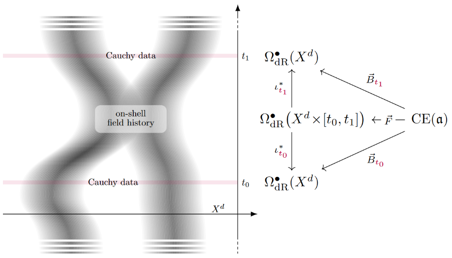
Next, assume a globally hyperbolic spacetime

X 1,d 1,0×X d X^{1,d} \simeq \mathbb{R}^{1,0} \times X^d

with Cauchy surface X dι t 1,0×X dX^d \xhookrightarrow{ \iota_t } \mathbb{R}^{1,0} \times X^d

and consider the time-local solution space

LocSol t{ temporal germs of solutions of the above EoMs around {t}×X d}. LocSol_t \;\coloneqq\; \left\{ \begin{array}{l} \text{ temporal germs of solutions } \\ \text{ of the above EoMs around }\; \{t\} \times X^d \end{array} \right\} \mathrlap{\,.}


Proposition.

Pullback to the Cauchy surface constitutes a bijection:

LocSol tι t *{B(B (i)Ω dR deg i(X d)) iI|dB=P(B)higher Gauss law} LocSol_t \xrightarrow[\sim]{\phantom{--}\iota_t^\ast\phantom{--}} \Big\{ \vec B \coloneqq \big( B^{(i)} \in \Omega^{deg_i}_{dR}(X^d) \big)_{i \in I} \;\Big\vert\; \overset{ \text{higher Gauss law} }{ \overbrace{ \mathrm{d}\vec B = \vec P(\vec B) } } \Big\}

so:


Proposition: Moreover:

The higher Gauss law is equivalently the closure (flatness)

condition of 𝔞\mathfrak{a}-valued differential forms

{B|dB=P(B)}Ω dR 1(X d;𝔞) cl \Big\{ \vec B \;\Big\vert\; \mathrm{d}\vec B = \vec P(\vec B) \Big\} \;\; \simeq \;\; \Omega^1_{dR}\big(X^d; \mathfrak{a}\big)_{cl}

for a characteristic L L_\infty-algebra 𝔞\mathfrak{a}

\linbreak

Let’s recall what this means:


connected L L_\infty-algebras of finite type are

L Alg conn ft CE dgcAlg op (𝔤,[],[,], [,,],) ( 𝔤 ,d | 1𝔤 =[] *+[,] *+ [,,] *+) \begin{array}{ccc} L_\infty Alg^{ft}_{conn} &\xhookrightarrow{\phantom{--}CE\phantom{--}}& dgcAlg^{op} \\ \left( \mathfrak{g} ,\; \begin{array}{l} [-], [-,-], \\ [-,-,-], \cdots \end{array} \right) &\mapsto& \left( \wedge^\bullet \mathfrak{g}^{\vee} ,\, \mathrm{d}_{\vert \wedge^1 \mathfrak{g}^{\vee}} = \begin{array}{l} [-]^\ast + [-,-]^\ast + \\ [-,-,-]^\ast + \cdots \end{array} \right) \end{array}

where 𝔤\mathfrak{g} is

and closed L L_\infty-valued forms are

Ω dR 1(X;𝔤) clHom dgAlg(CE(𝔤),Ω dR (X)) \Omega^1_{dR}\big(X; \mathfrak{g}\big)_{cl} \;\coloneqq\; Hom_{dgAlg}\Big( CE(\mathfrak{g}) , \Omega^\bullet_{dR}(X) \Big)


Example/Definition/Proposition

For 𝒜\mathcal{A} a connected topological space

with abelian fundamental groups (for simplicity)

and dim (H (𝒜,))<dim_{\mathbb{R}}\big(H^\bullet(\mathcal{A},\mathbb{R})\big) \lt \infty,

then its real Whitehead L∞-algebra 𝔩𝒜\mathfrak{l}\mathcal{A} is

(𝔩𝒜) π (Ω𝒜) (\mathfrak{l}\mathcal{A})_\bullet \coloneqq \pi_\bullet(\Omega \mathcal{A}) \otimes_{\mathbb{Z}} \mathbb{R}

with brackets uniquely determined by the condition that

H (CE(𝔩𝒜))H (𝒜;). H^\bullet\big( CE(\mathfrak{l}\mathcal{A}) \big) \;\simeq\; H^\bullet\big( \mathcal{A}; \mathbb{R} \big) \mathrlap{\,.}


Examples

electromagnetism: 𝔞=𝔩(BU(1) 2)\mathfrak{a} = \mathfrak{l}(B \mathrm{U}(1)^2)

self-dual higher gauge field: 𝔞=𝔩B 2k\mathfrak{a} = \mathfrak{l} B^{2k} \mathbb{Z}

RR-field: 𝔞=𝔩(BU)\mathfrak{a} = \mathfrak{l}(B \mathrm{U})

Maxwell-Chern-Simons field: 𝔞=𝔩S 2\mathfrak{a} = \mathfrak{l}S^2

C-field: 𝔞=𝔩S 4\mathfrak{a} = \mathfrak{l}S^4


Definition/Proposition.

The total flux of a flux density F\vec F

is its image in non-abelian de Rham cohomology

H dR 1(X;𝔞)Ω dR 1(X;𝔞) cl/concordance H^1_{dR}\big( X;\, \mathfrak{a} \big) \;\simeq\; \Omega^1_{dR}\big(X; \mathfrak{a}\big)_{cl}\big/ \text{concordance}


Definition/Proposition.

Denoting by

  • L 𝒜L^{\mathbb{Q}}\mathcal{A} the rationalization of 𝒜\mathcal{A},

  • L 𝒜L^{\mathbb{R}}\mathcal{A} its extension of scalars to the reals

  • η :𝒜L 𝒜\eta^{\mathbb{R}} \colon \mathcal{A} \longrightarrow L^{\mathbb{R}} \mathcal{A} the comparison map,

the nonabelian character map is

charge in nonabelian cohomology character total flux in nonabelian dR-cohomology H 1(X;Ω𝒜) ch 𝒜 H dR 1(X;𝔞) = π 0Map(X,𝒜) η π 0Map(X,L 𝒜) \begin{array}{ccc} \begin{array}{c} \text{charge in} \\ \text{nonabelian cohomology} \end{array} &character& \begin{array}{c} \text{total flux in} \\ \text{nonabelian dR-cohomology} \end{array} \\ H^1(X;\,\Omega \mathcal{A}) &\xrightarrow{\phantom{--} ch^{\mathcal{A}} \phantom{--}}& H^1_{dR}\big(X;\,\mathfrak{a}\big) \\ = && \simeq \\ \pi_0\, Map\big(X, \mathcal{A}\big) &\xrightarrow{\phantom{--} \eta^{\mathbb{R}} \phantom{--}}& \pi_0\, Map\big(X, L^{\mathbb{R}}\mathcal{A}\big) \end{array}


Flux quantization of a higher gauge theory is

choice of 𝒜\mathcal{A} with 𝔩𝒜𝔞\mathfrak{l}\mathcal{A}\simeq \mathfrak{a}

Promotion of flux densities to pairs (F,χ)(\vec F, \chi) for

χ\chi a charge whose character is the total flux of F\vec F:

Ω dR 1(X d;𝔞) cl [] H dR 1(X d;𝔞) ch 𝒜 H 1(X d;Ω𝒜) F [F]=ch 𝒜([χ]) | [χ] \begin{array}{ccccc} \Omega^1_{dR}\big( X^d; \mathfrak{a} \big)_{cl} &\xrightarrow{ [-] }& H^1_{dR}\big( X^d;\, \mathfrak{a} \big) &\xleftarrow{ ch^{\mathcal{A}} }& H^1(X^d; \Omega \mathcal{A}) \\ \vec F &\mapsto& [\vec F] = ch^{\mathcal{A}}([\chi]) &\leftarrow\!\!\!\vert& [\chi] \end{array}


There are either none or infinitely many admissible 𝒜\mathcal{A}

\Rightarrow 𝒜\mathcal{A} is a hypothesis about the correct model for given physics


Examples

Dirac charge quantization of EM-field: 𝒜BU(1) 2\mathcal{A} \equiv B \mathrm{U}(1)^2

Hypothesis K on the RR-field

Hypothesis h on Maxwell-Chern-Simons field: 𝒜S 2\mathcal{A} \equiv S^2

Hypothesis H on C-field: 𝒜S 4\mathcal{A} \equiv S^4


Finally, the full completed higher gauge field

is not just the flux densities F\vec F, a charge χ\chi

and an equality [F]=ch[χ][\vec F] = ch[\chi], but involves

a gauge transformation/homotopy A^\widehat{A} exhibiting this equality

which out the “be” the gauge potentials.

The globally completed phase space is, schematically:

PhsSpc{flux densities FΩ dR 1(X d;𝔞) cl local charges χMap(X d,𝒜) gauge potentials A^:Fχ} PhsSpc \;\coloneqq\; \left\{ \begin{array}{ll} \text{flux densities} & \vec F \in \Omega^1_{dR}(X^d;\mathfrak{a})_{cl} \\ \text{local charges} & \chi \in Map(X^d, \mathcal{A}) \\ \text{gauge potentials} & \widehat{A} \colon \vec F \Rightarrow \chi \end{array} \right\}


More in detail, this is the smooth ∞-groupoid

which as such is the homotopy pullback

of the character map from total flux to flux densities.


Essentially. In the following we will only need

the shape of the space space,

which turns out to be given by a concrete formula.


Part 2 – Their Complete Topological Quantization


observables are the smooth functions on phase space

O:PhsSpc O \,\colon\, PhsSpc \longrightarrow \mathbb{C}

the topological observables are the locally constant functions

O top:PhsSpc O_{top} \,\colon\, PhsSpc \longrightarrow \flat \mathbb{C}

(where 𝒞\flat \mathcal{C} is the discrete set underlying 𝒞\mathcal{C})


Proposition

The topological observables

PhsSpc PhsSpc \xrightarrow{\phantom{--}} \flat \mathbb{C}

are naturally equivalent to the maps

π 0Map(X d,𝒜)𝒞 \pi_0 \, Map(X^d, \mathcal{A}) \xrightarrow{\phantom{--}} \mathcal{C}

out of the connected components of the mapping space

from the Cauchy surface into the classifying space,


“Topologically, fields are only seen through their charges.”


Moreover, realistic observables are

supported on finitely many components, hence:

TopObs[π 0Map(X d,𝒜)]H 0(Map(X d,𝒜);) TopObs \;\coloneqq\; \mathbb{C}\big[ \pi_0 \, Map(X^d, \mathcal{A}) \big] \,\simeq\, H_0\big( Map(X^d, \mathcal{A}) ;\, \mathbb{C} \big)


More specifically, we look at field solitons,

whose charge vanishes at infinity


To formalize this, consider a pointed topological space

(X dom d,)Top * \big( X^d_{dom}, \infty \big) \in Top^\ast

with basepoint thought of as a point at infinity:

X dX dom d{} X^d \,\simeq\, X^d_{dom} \setminus \{\infty\}


Also think of 𝒜\mathcal{A} as pointed by 0-charge

(𝒜,0)Top *. \big(\mathcal{A}, 0\big) \in Top^\ast \,.


Then a pointed map χMap *(X dom d,𝒜)\chi \in Map^\ast\big(X^d_{dom}, \mathcal{A}\big)

literally takes the value 00 at \infty

X dom d χ 𝒜 {} {0} \begin{array}{ccc} X^d_{dom} &\xrightarrow{\phantom{--} \chi \phantom{--}}& \mathcal{A} \\ \uparrow && \uparrow \\ \{\infty\} &\xrightarrow{\phantom{----}}& \{0\} \end{array}


So the solitonic topological observabels are

TopObs[Map *(X dom d,𝒜)] TopObs \,\coloneqq\, \mathbb{C}\Big[ Map^\ast\big(X^d_{dom}, \mathcal{A}\big) \Big]


Question: What is the quantum operator product \star on TopObsTopObs?

Feynman 1948: the time-ordered ordinary product

e.g. for field operators ϕ\phi and their canonical momenta:

π(t,x)ϕ(t,y) = limϵ +0π(t+ϵ,x)ϕ(t,y) ϕ(t,x)π(t,y) limϵ +0ϕ(t+ϵ,x)π(t,y) \begin{array}{rcr} \big\langle \pi(t, \vec x) \star \phi(t, \vec y) \big\rangle &=& \underset{\underset{\epsilon \to_+ 0}{\longrightarrow}}{\lim} \big\langle \pi(t + \epsilon, \vec x) \cdot \phi(t, \vec y) \big\rangle \\ - \big\langle \phi(t, \vec x) \star \pi(t, \vec y) \big\rangle && - \underset{\underset{\epsilon \to_+ 0}{\longrightarrow}}{\lim} \big\langle \phi(t + \epsilon, \vec x) \cdot \pi(t, \vec y) \big\rangle \end{array}


NB: The analogue is still true for light front quantization

with respect to ordering in the light-front parameter x +x 0+x 1x^+ \coloneqq x^0 + x^1.


So consider light-front quantization on spacetime if the form

X 1,d 1,1×X d1 X d 1×X d1 X dom d = {} 1X dom d1 \begin{aligned} X^{1,d} &\simeq\, \mathbb{R}^{1,1} \times X^{d-1} \\ X^d & \simeq \mathbb{R}^1 \times X^{d-1} \\ X^d_{dom} & = \mathbb{R}^1_{\cup \{\infty\}} \wedge X^{d-1}_{dom} \end{aligned}


For topological observables which are necessarily x 0x^0-independent

their light-front ordering is their x 1x^1-ordering.

This is given by the Pontrjagin product/fundamental group algebra-structure on:

TopObs =H 0(Map *( {} 1X dom d)) H 0(ΩMap *(X dom d)) [π 1Map *(X dom d)] \begin{aligned} TopObs & = H_0\Big( Map^\ast\big( \mathbb{R}^1_{\cup \{\infty\}} \wedge X^d_{dom} \big) \Big) \\ & \simeq H_0\Big( \Omega Map^\ast\big( X^d_{dom} \big) \Big) \\ & \simeq \mathbb{C}\Big[ \pi_1 \, Map^\ast\big( X^d_{dom} \big) \Big] \end{aligned}

induced under pushforward in homology

H 0(ΩM)H 0(ΩM)H 0(ΩM×ΩM) *H 0(ΩM) H_0(\Omega M) \otimes H_0(\Omega M) \simeq H_0(\Omega M \times \Omega M) \xrightarrow{\phantom{--} \star_\ast \phantom{--}} H_0(\Omega M)

from concatenation of loops

ΩM×ΩM ΩM ( 2, 1) 2 1 :x 1{ 1(ln(1x 1)) | x 10 2(ln(+x 1)) | x 10 \begin{array}{ccc} \Omega M \times \Omega M &\xrightarrow{\phantom{--} \star \phantom{--}}& \Omega M \\ \big( \ell_2, \ell_1 \big) &\mapsto& \ell_2 \star \ell_1 & \colon\; x^1 \,\mapsto\, \left\{ \begin{array}{lcl} \ell_1\big(\ln(-\tfrac{1}{x^1})\big) & \vert & x^1 \geq 0 \\ \ell_2\big(\ln(+x^1)\big) & \vert & x^1 \leq 0 \end{array} \right. \end{array}


So where δ TopObs\delta_\ell \in TopObs
is the {0,1}\{0,1\}-valued observable asking:

“Is the field history of shape [][\ell]?”

the observable δ 2δ 1\delta_{\ell_2} \star \delta_{\ell_1} asks

“Is the field history
first of shape 1\ell_1 and
then of shape 2\ell_2?”


With the algebra of topological quantum observables understood,

the topological quantum states are its modules,

which here are the linear representations of the moduli fundamental group:

TopQuStSpc (TopObs,)Mod (H 0(ΩMap *(X dom d1,𝒜)),)Mod ([π 1Map *(X dom d1,𝒜)])Mod (π 1Map *(X dom d1,𝒜))Rep \begin{aligned} TopQuStSpc & \coloneqq (TopObs, \star) Mod \\ & \equiv \Big( H_0\big( \Omega Map^\ast(X^{d-1}_{dom}, \mathcal{A}) \big), \star \Big) Mod \\ & \simeq \Big( \mathbb{C}\big[ \pi_1 Map^\ast(X^{d-1}_{dom}, \mathcal{A}) \big] \Big) Mod \\ & \simeq \big( \pi_1 Map^\ast(X^{d-1}_{dom}, \mathcal{A}) \big) Rep \end{aligned}


Part 3 – Application to Topological Quantum Materials


Consider 𝔤\mathfrak{g}-Yang-Mills theory on

X 1,3= 1,1×Σ 2 X^{1,3} = \mathbb{R}^{1,1} \times \Sigma^2

What are its standard topological flux quantum observables?


Proposition.

The Poisson brackets on linear E/M YM-flux observables through Σ 2\Sigma^2 are:

C (Σ 2,𝔤 )electric flux adC (Σ 2,𝔤 0),magnetic flux \underset{\text{electric flux}}{ \underbrace{ C^\infty\big( \Sigma^2, \mathfrak{g}_{\hbar} \big) } } \ltimes_{ad} \underset{\text{magnetic flux}}{ \underbrace{ C^\infty\big( \Sigma^2, \mathfrak{g}_{0} \big) } \mathrlap{\,,} }

where 𝔤 \mathfrak{g}_{\hbar} is 𝔤\mathfrak{g} with Lie bracket rescaled by >0\hbar \in \mathbb{R}_{\gt 0}.

Their non-perturbative C-star algebraic deformation quantization

is the C *C^\ast-convolution algebra:

[C (Σ 2,G) AdC (Σ 2,𝔤 0/Λ)] \mathbb{C}\Big[ C^\infty\big( \Sigma^2, G \big) \ltimes_{Ad} C^\infty\big( \Sigma^2, \mathfrak{g}_{0}/\Lambda \big) \Big]

for choices of


Hence the traditional non-perturbative topological quantum observables

on E/M Yang-Mills fluxes through a surface Σ 2\Sigma^2 are:

TopObs trad =[π 0C (Σ 2,G𝔤 0/Λ)] [π 0Map(Σ 2,G𝔤 0/Λ)] [π 1Map(Σ 2,B(G𝔤 0/Λ))] \begin{aligned} TopObs^{trad} & = \mathbb{C}\Big[ \pi_0 C^\infty\big( \Sigma^2, G \ltimes \mathfrak{g}_{0}/\Lambda \big) \Big] \\ & \simeq \mathbb{C}\Big[ \pi_0 Map\big( \Sigma^2, G \ltimes \mathfrak{g}_{0}/\Lambda \big) \Big] \\ & \simeq \mathbb{C}\Big[ \pi_1 Map\big( \Sigma^2, B(G \ltimes \mathfrak{g}_{0}/\Lambda) \big) \Big] \end{aligned}

Specifically for Maxwell theory, where 𝔤=𝔲(1)\mathfrak{g} = \mathfrak{u}(1),

if we choose G=U(1)G = \mathrm{U}(1) and Λ=\Lambda = \mathbb{Z} \subset \mathbb{R} then

TopObs trad=[π 1Map(Σ 2,BU(1) 2)] TopObs^{trad} = \mathbb{C}\Big[ \pi_1 Map\big( \Sigma^2, B \mathrm{U}(1)^2 \big) \Big]

which coincides with our general TopObsTopObs from above.


Example.

For Σ 2=T 2\Sigma^2 = T^2 the 2-torus,

π 1Map(T 2,BU(1)) π 0Map(T 2,U(1)) H 1(T 2;) a× b \begin{aligned} \pi_1 Map\big( T^2 , B \mathrm{U}(1) \big) & \simeq \pi_0 Map\big( T^2 , \mathrm{U}(1) \big) \\ & \simeq H^1(T^2; \mathbb{Z}) \\ & \simeq \mathbb{Z}_a \times \mathbb{Z}_b \end{aligned}

Algebra of Maxwell Wilson loops on torus.


Now consider lifting these particles in 4D to strings in 5D

X 1,4 1,1×( 1×Σ 2) X^{1,4} \simeq \mathbb{R}^{1,1} \times (\mathbb{R}^1 \times \Sigma^2)

X dom 4= {} 1( 1×Σ 2) . X^4_{dom} = \mathbb{R}^1_{\sqcup \{\infty\}} \wedge (\mathbb{R}^1 \times \Sigma^2)_{\cup \infty} \,.


Under Hyothesis h, with 𝒜=S 2ι 2BU(1)\mathcal{A} = S^2 \xhookrightarrow{\iota_2} B \mathrm{U}(1),

the topological observables are deformed to:

Proposition.

π 1Map(T 2,S 2) 2^ \pi_1 Map\big( T^2, S^2 \big) \simeq \widehat{\mathbb{Z}^2}

which is the integer Heisenberg group at level=2:

2^ Set( a× b)× \widehat{\mathbb{Z}^2} \coloneqq_{Set} (\mathbb{Z}_a \times \mathbb{Z}_b) \times \mathbb{Z}

with generating elements

W a ((1,0),0) W b ((0,1),0) ζ ((0,0),1) \begin{aligned} W_a &\coloneqq \big((1,0), 0\big) \\ W_b &\coloneqq \big((0,1), 0\big) \\ \zeta &\coloneqq \big((0,0), 1\big) \end{aligned}

on which the only non-trivial group commutator is

[W a,W b]=ζ 2. [W_a, W_b] = \zeta^2 \mathrlap{\,.}


This is a nonabelian deformation of the Maxwell Wilson loops.

In fact this is exactly the algebra of observables of:

  1. abelian Chern-Simons theory

  2. anyons in fractional quantum Hall systems,

the latter being (vortices in a 2D electron liquid induced by)

surplus magnetic flux quanta

on top of some rational number of flux quanta per electrons.


Let’s further lift this situation to 11D supergravity on

X 1,10 1,3×( 1×S 3×S 3) X^{1,10} \coloneqq \mathbb{R}^{1,3} \times \big( \mathbb{R}^1 \times S^3 \times S^3 \big)

with

X dom 10 {} 3( 1×S 3×S 3) {} X^{10}_{dom} \coloneqq \mathbb{R}^3_{\sqcup \{\infty\}} \wedge \big( \mathbb{R}^1 \times S^3 \times S^3 \big)_{\cup \{\infty\}}

globally completed according to Hypothesis H:


Proposition.

π 1Map(S 3×S 3,S 4) 2^× /12 \pi_1 Map\big( S^3 \times S^3, S^4 \big) \simeq \widehat{\mathbb{Z}^2} \times \mathbb{Z}_{/12}

Under the Pontrjagin theorem this says that

5-branes on this background, wrapped on 1,3\mathbb{R}^{1,3}

have the same anyon braiding in S 3×S 3S^3 \times S^3 as FQH anyons on T 2T^2


Back to the case in 5D,

to see more transparently where the anyon braiding comes from

consider the simpler situation flux through the plane

X 1,4 = 1,1×( 1× 2) X dom 4 = {} 1 3 \begin{aligned} X^{1,4} & = \mathbb{R}^{1,1} \times (\mathbb{R}^1 \times \mathbb{R}^2) \\ X^4_{dom} & = \mathbb{R}^1_{\sqcup \{\infty\}} \wedge \mathbb{R}^3_{\cup \infty} \end{aligned}

Then the 2-Cohomotopical quantum observables are spanned by

π 1Map(S 2,S 2)π 3(S 2) \pi_1 \, \mathrm{Map}\big( S^2 ,\, S^2 \big) \simeq \pi_3(S^2) \simeq \mathbb{Z}

This looks simple, but let’s see what these observables observe:

Pontrjagin theorem:

π 2(S 3)={framed links}/(cobordism) \pi^2(S^3) = \Big\{ \text{framed links} \Big\} \Big/ \big(\text{cobordism}\big)

In our situation, these links are

vacuum diagrams of flux quanta on the surface.


Proposition.

The observables

{framed links} L #L \begin{array}{ccc} \Big\{ \text{framed links} \Big\} &\longrightarrow& \mathbb{Z} \\ L &\mapsto& \# L \end{array}

compute the writhe or total linking of a link.

Hence in a pure quantum state |K\vert K \rangle this is

K|𝒪 L|K =exp(πiK#L) =exp(πiK( ijlnk(L i,L j)+ ifrm(L i))) \begin{aligned} \langle K \vert \mathcal{O}_L \vert K \rangle & = \exp\big( \tfrac{\pi \mathrm{i}}{K} \# L \big) \\ & = \exp\bigg( \tfrac{\pi\mathrm{i}}{K} \Big( \textstyle{\sum_{i \neq j}} lnk(L_i, L_j) + \textstyle{\sum_{i}} frm(L_i) \Big) \bigg) \end{aligned}

These are exactly the expectation values of traditionally

renormalized Wilson loop observable of abelian Chern-Simons.


The first line shows that a braiding phase

ζexp(πiK) \zeta \coloneqq \exp(\tfrac{\pi \mathrm{i}}{K})

is picked up for each crossing in the link diagram

hence for each braiding of the anyon worldlines.


For more see at ncatlab.org/schreiber/show/ICMS25


Last revised on April 9, 2026 at 09:23:05. See the history of this page for a list of all contributions to it.