nLab geometry of physics -- flux quantization

under construction

this page is based on the MathPhys Encyclopedia-entry SS24

this entry is one section of “geometry of physics”

previous section: fundamental super p-branes

Abstract.

For higher gauge fields of Maxwell type — e.g. the common electromagnetic field (the “A-field”) but also the B-, RR-, and C-fields considered in string/M-theory — flux&charge-quantization laws specify non-perturbative completions of these fields by encoding their solitonic behaviour and hence by specifying the quantized charges carried by the individual branes that source these fluxes (higher-dimensional monopoles or solitons).

This page surveys the general (rational-)homotopy theoretic understanding [FSS23-Char] of flux- & charge-quantization via the Chern-Dold character map generalized to the non-linear (self-sourcing) Bianchi identities that appear in higher-dimensional supergravity theories, notably for B-&RR-fields in D=10 supergravity and for the C-field in D=11 supergravity.

History.

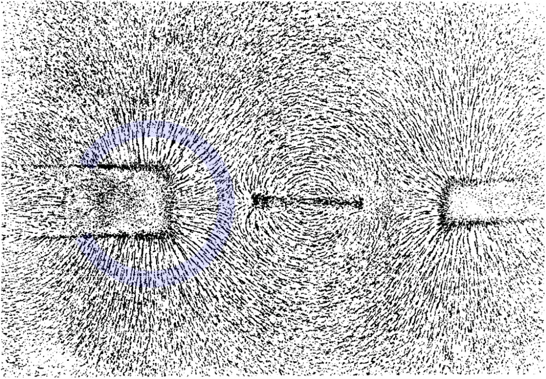
In 1852 Faraday observes magnetic field flux lines emanating from magnetic poles [Faraday 1852].

In 1931 Dirac invokes quantum mechanics to argue that, if there were unpaired such (mono-)poles, then the total flux emanating from them — and thus the magnetic charge carried by them — had to come in integer multiples of a unit quantum [Dirac 1931].

In 1957 Abrikosov essentially notices that the same electromagnetic flux-&charge-quantization mechanism makes vortex strings in type II superconductors carry units of localized magnetic flux. [Abrikosov 1957]

In 1985 Alvarez understands such solitonic magnetic fields as 2-cocycles in (differential) ordinary cohomology. [Alvarez 1985]

In 1988 Gawędzki observes that the B-field flux felt by a string must similarly be quantized as a 3-cocycle in Deligne cohomology. [Gawędzki 1988, also Freed & Witten 1999]

In the 1990s string theorists hypothesize that the combined flux of B-&RR-fields and hence the charge of D-branes is analogously quantized in a generalized cohomology theory called “topological K-theory” [Minasian & Moore 1997; Witten 1998] or more generally in “twisted” such K-theory [Bouwknegt & Mathai 2001],

and that the flux of the C-field and hence the charge of M-branes is quantized in a “shifted half-integral” cohomology theory [Witten 1996] whose proper mathematical home motivates Hopkins & Singer 2005 but remains somewhat mysterious, for a long time.

In the 2020s Fiorenza et al. 2020 develop a systematic understanding [FSS23-Char] of flux quantization of any higher gauge theory of Maxwell-type in generalized non-abelian cohomology theory, using tools from dg-algebraic rational homotopy theory related to the "FDA-method" in the supergravity literature.

This provides a transparent re-derivation of known flux quantization laws and it allows to finally discuss C-field flux- and M-brane charge-quantization.

Overview

(§2) A higher gauge theory (review includes Alfonsi 2024, §2; BFJ${}^+$ 2024) of Maxwell-type (Def. below) is a (quantum) field theory analogous to vacuum-electromagnetism (on curved spacetimes), but with the analog of the electromagnetic flux density $F_2$ (which ordinarily is a differential 2-form on 3+1 dimensional spacetime $X^4$) allowed to be a system of differential forms $\vec F \,\equiv\, \big\{F^{(i)}\big\}_{i \in I}$ of any degree $deg_i \geq 1$ on a $D$-dimensional spacetime $X^D$ of any dimension $D = d+1 \geq 2$, and satisfying a higher analog of Maxwell's equations (6).

Such higher gauge theories famously appear as the gauge field-sector in higher-dimensional supergravity and hence in super-string/M-theory, which is where they draw most of their motivation from.

In analogy to how for ordinary Maxwell theory one may think of singularities or stable bumps in the flux density $F_2$ as being sourced by charges carried by (hypothetical) Dirac monopoles or by (observed) Abrikosov vortex strings, respectively, so one may think of singularities or stable bumps in these higher flux densities as sourced by singular branes or solitonic branes, respectively, for suitably higher dimensional (mem-)branes carrying suitable higher charges.

(§3) But for such singular/solitonic branes to be “elementary” objects of individually discernible nature, their charges, and hence the total fluxes which they source, should have discrete (“quantized”) values (as indeed observed for Abrikosov vortex strings). This is what flux quantization is about.

Traditionally one declares the full higher gauge field to be given by gauge potentials $\widehat A$ whose curvature is the flux density $\vec F$ and which is globally subjected to a topological condition that implies the flux and charge quantization. While this is classical for electromagnetism (and Yang-Mills theory), it is not transparent from this point of view how to identify the structure of gauge potentials for general higher gauge theories.

More systematically, one may understand flux quantization as the specification of a generalized (non-abelian) cohomology theory for which the charges are required to be cocycles, and of which the total fluxes are then the differential-geometric (Chern-Dold-)characters.

From this streamlined point of view the higher gauge potential, and hence the full field content of the higher gauge theory, arises as the homotopy/gauge theoretic witness of the matching of total fluxes with the character of the charges, making the full higher gauge fields be cocycles in a corresponding generalized (nonabelian) differential cohomology theory.

(§4) Examples of flux quantization beyond Dirac charge quantization in electromagnetism play a key role in string/M-theory:

• the seminal “Hypothesis K” postulating D-brane charge quantization in K-theory,

• the more recent “Hypothesis H” postulating M-brane charge quantization in unstable twisted Cohomotopy.

These hypotheses are not unrelated: Under “double dimensional Kaluza-Klein reduction” along a circle fiber, the C-field fluxes on $X^{10+1}$ are to give rise to most of the $B$-/RR-field-fluxes in $X^{9+1}$ (as part of the duality between M-theory and type IIA string theory, which is either conjectural or defining, depending on attitude towards the definition of the elusive M-theory). Therefore Hypothesis H may be understood as providing an non-perturbative/M-theoretic lift of Hypothesis K to the extent that it reduces to the latter under double dimensional reduction, and as a non-perturbative/M-theoretic correction to the extent that it does not quite reduce to Hypothesis K.

Perspective. This highlights that a choice of flux quantization is (depending on perspective of how that higher gauge theory is ultimately defined):

• a hypothesis about

or else

• a specification of

the non-perturbative completion of the given higher gauge theory, which is generally an issue that deserves (more) attention.

Traditionally, flux quantization laws have been postulated sporadically and in ad-hoc fashion, in order to patch up “anomalous” theories: Since the ancient past it has been common to define any physical theory by a stationary action principle embodied by a Lagrangian density, from which a perturbative BRST complex is extracted, whose quantization (e.g. Henneaux & Teitelboim 1992) is generally afflicted with problems (“anomalies”) some of which are dealt with by ad-hoc flux quantization: For example the original Dirac charge quantization was postulated to cure an anomaly in the quantum theory of an electron propagating in the background field of a magnetic monopole (a “0-brane”), while the enigmatic shifted C-field flux quantization similarly serves to cure an anomaly in the quantum theory of the M2-brane propagating in the background field of an M5-brane (Witten 1996a, §2.2).

More systematically, the available choices of flux-quantization laws $\mathcal{A}$ are algebro-topologically determined by the form of the higher Gauss law on any Cauchy surface, and any such choice, given by a compatible non-abelian cohomology-theory, determines the non-perturbative phase space stack of flux-quantized gauge fields. This process makes no reference to Lagrangian densities and applies seamlessly to field theories that do not even have a natural Lagrangian description, such as self-dual higher gauge theories.

Typically there is an “evident” choice of flux quantization and this is the choice tacitly made in the literature, where considered at all. But it is important to notice that there are other admissible choices, embodying hypotheses about (or definitions of) non-evident nonperturbative completions of the given higher gauge theory.

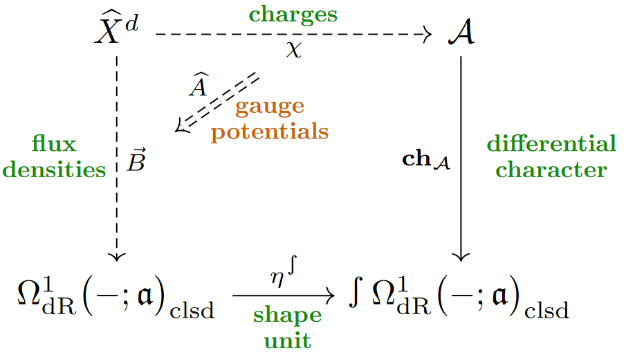
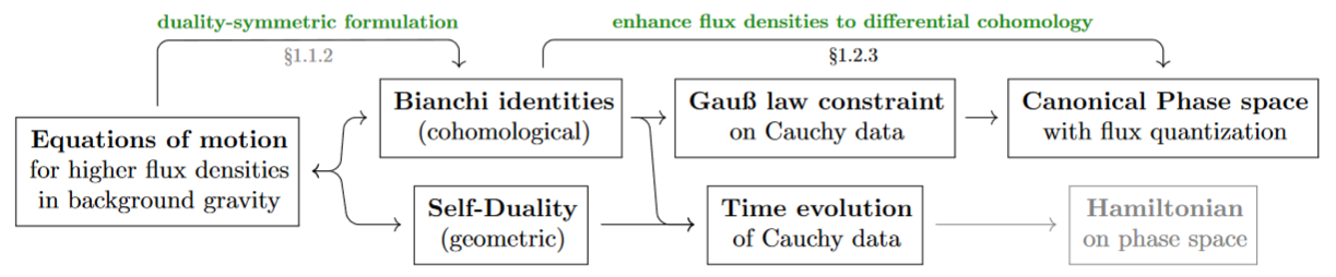
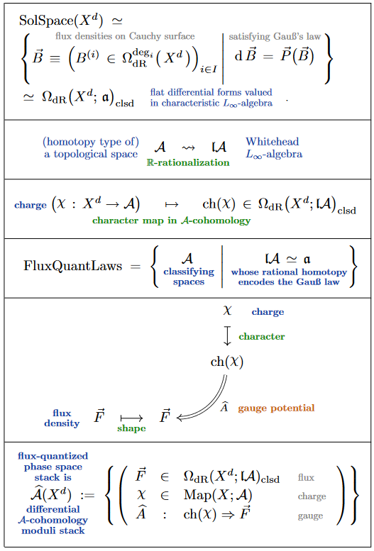
The logic of flux quantization. The following table shows in outline the logic of algebro-topological flux quantization as reviewed here; on the left in generality and on the right for our running examples:

1. traditional Dirac charge quantization of the electromagnetic field (experimentally well-supported);

2. traditional D-brane charge quantization in twisted topological K-theory (“Hypothesis K”);

3. more recent M-brane$\;$charge quantization in unstable twisted Cohomotopy (“Hypothesis H”).

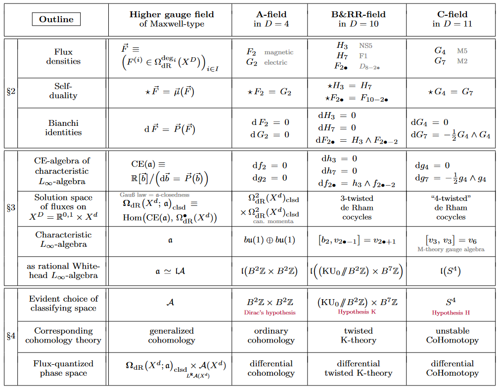
As this table indicates, the algebro-topological nature of flux/charge quantization is higher Lie theoretic (explained in §3), by matching two $L_\infty$-algebras associated with a given higher gauge theory of Maxwell type (§2):

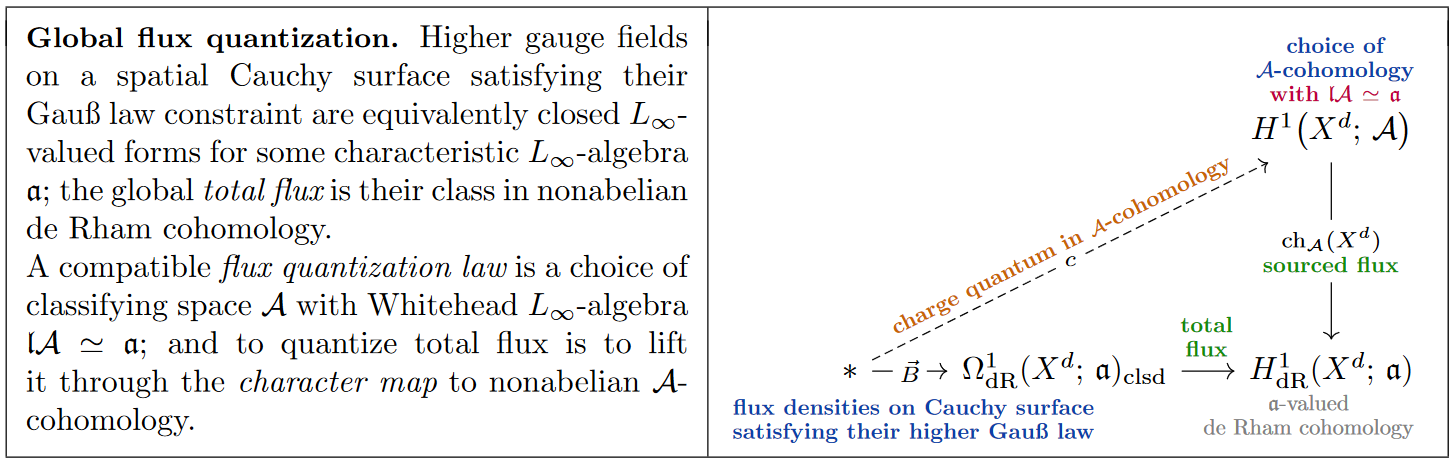
(i) Bianchi-Gauss $L_\infty$-algebras. The higher Bianchi identities of duality-symmetric higher flux densities, and hence their their higher Gauss law (Prop. ) are equivalent to the condition that the flux densities jointly constitute a closed $L_\infty$-algebra valued differential form with coefficients in a characteristic $L_\infty$-algebra $\mathfrak{a}$ (Prop. below):

(ii) Whitehead $L_\infty$-algebras. The classifying space $\mathcal{A}$ of any charge quantization law is rationally characterized by its rational Whitehead $L_\infty$-algebra $\mathfrak{l}\mathcal{A}$ (essentially the “Quillen model” of $\mathcal{A}$: that $L_\infty$-algebra whose Chevalley-Eilenberg algebra $CE(\mathfrak{l}\mathcal{A})$ is the Sullivan model of $\mathcal{A}$) and the nonabelian Chern-Dold character map extracts from $\mathcal{A}$-cohomology its image in $\mathfrak{l}\mathcal{A}$-valued nonabelian de Rham cohomology (27):

The admissible flux quantization laws for a higher gauge theory with Bianchi-Gauss $L_\infty$-algebra $\mathfrak{a}$ are hence those classified by spaces $\mathcal{A}$ with Whitehead $L_\infty$-algebra $\mathfrak{l}\mathcal{A} \simeq \mathfrak{a}$. Given such a choice, then quantizing a flux density $\vec B$ is to lift its $\mathfrak{a}$-valued de Rham-class to a class in $\mathcal{A}$-valued nonabelian cohomology.

More in detail, a flux-quantized higher gauge field is (i) a flux density $\vec B$ being a cocycle in $\mathfrak{a}$-de Rham cohomology, (ii) a charge $\rchi$ being a cocycle in $\mathcal{A}$-cohomology and (iii) a gauge potential $\widehat A$ being a coboundary between their joint images (thus exhibiting the above identification of their cohomology classes).

This makes the flux-quantized higher gauge fields be cocycles in differential $\mathcal{A}$-cohomology.

In the following we discuss all this in more detail.

Remark

(the role of $L_\infty$-algebras: curvature-coefficients instead of gauge potiential-coefficients)
In comparison to more traditional discussions, beware that the (possibly non-abelian) $L_\infty$-algebra $\mathfrak{a}$ here controls the (possibly non-linear) Bianchi identities/Gauss law satisfied by the curvature forms/flux densities — and thus is not the (higher) Lie algebra in which the gauge potentials take values, if any. (Even in the abelian case, where both types of coefficient $L_\infty$-algebras make sense, they differ by a degree-shift.)

This is an underappreciated use of $L_\infty$-algebras in physics, but it is known from the “FDA”-method in supergravity and is tacitly familiar in traditional discussion of RR-flux/D-brane charge:

Here the characteristic $L_\infty$-algebra $[b_2, \, v_{2\bullet-1}] = v_{2\bullet + 1}$ bears no resemblance to the Lie algebra $\mathfrak{su}(n)$, and yet after choosing D-brane charge quantization in topological K-theory it follows (an algebro-topological form of “gauge enhancement”) that gauge potentials with coefficients in $\mathfrak{su}(n)$ (namely connections on Hermitean vector bundles) provide cocycles for the resulting differential K-theory. It is in this way (RR-flux quantization $\rightsquigarrow$ K-theory $\rightsquigarrow$ gauge bundles as cocycles) that non-abelian gauge fields appear on D-branes.

In fact, flux quantization as discussed here does not apply to $\mathfrak{su}(n)$-Yang-Mills theory directly:

Generally, not all $L_\infty$-algebras appear as rational Whitehead $L_\infty$-algebras of (the homotopy type (37) of) a topological space $\mathcal{A}$ that is amenable to rationalization; those that do are “nilpotent”. Specifically, $\mathfrak{su}(n)$ ($n \geq 2$) is not a nilpotent Lie algebra, which relates to the fact that flux quantization as discussed here — while it does apply to non-linear/non-abelian higher Bianchi identities such as for the C-field — does not apply directly to Yang-Mills theory with gauge Lie algebra $\mathfrak{su}(n)$ (or other classical Lie algebras).

Flux densities and Brane charges

Electromagnetic flux and its “branes”

Faraday observed “lines of force” – now called flux of the magnetic field – concentrating towards the poles of rod magnets:

From Faraday’s diary of experimental investigation, vol VI, entry from 11th Dec. 1851, as reproduced in Martin 2009, p. 311 -- the colored arc is our addition, for ease of comparison with the next graphics.

In modern differential-geometric formulation, the density of these flux lines through any given surface-element is encoded in a differential 2-form $F_2$, as indicated in the following schematic graphics:

adapted from Hyperphysics

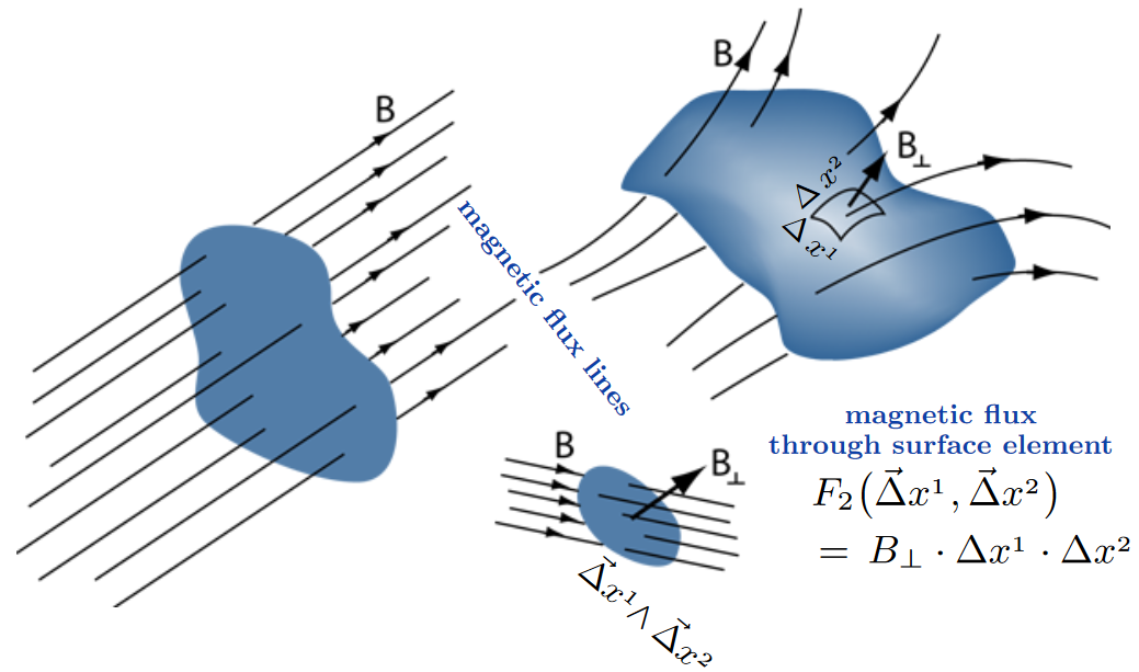
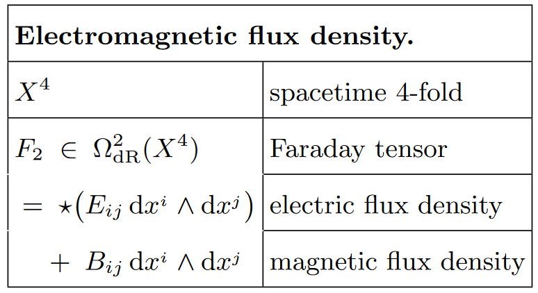
More in detail, with respect to any foliation $X^4 \simeq \mathbb{R}^1 \times X^3$ of a globally hyperbolic spacetime $X^4$ by spacelike Cauchy surfaces $X^3$, the spatial component of $F_2$ is the magentic flux density $B$, while the Hodge dual (with respect to $X^4$) of the temporal component is the electric flux density $E$.

Imagining, as Dirac did, that Faraday’s rod magnet could be made infinitely long and thin, any one of its poles would look like an isolated mono-pole with flux concentrating towards it from all directions:

(1)

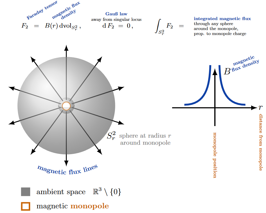
At the point of the idealized monopole itself, the flux density $B$ per unit volume would diverge – a “singularity” much in the sense of black holes, which therefore we do not regard to be part of space(-time): The spacetime domain on which to discuss the fluxes sourced by a magnetic monopole is (more on this below) not Minkowski spacetime $\mathbb{R}^{3,1}$ itself, but its complement around the worldline $\mathbb{R}^{0,1}$ of the would-be monopole:

$$\mathbb{R}^{3,1} \setminus \mathbb{R}^{0,1} \; \underset{\mathrm{homeo}}{\simeq} \; \mathbb{R}^{0,1} \times \big( \mathbb{R}^3 \setminus \{0\} \big) \; \underset{\mathrm{homeo}}{\simeq} \; \mathbb{R}^{0,1} \times R^1_{\gt 0} \times S^2 \; \underset{\mathrm{hmtp}}{\simeq} \; S^2 \,.$$

As such, magnetic monopoles are the singular 0-branes of electromagnetism (cf. below) — in theory: Whether magnetic monopoles exist in nature remains open; they have not been seen in experiment, but there are decent theoretical arguments that they should exist if the standard model symmetry is a broken symmetry grand unified symmetry.

On the other hand, the “solitonic branes” of electromagnetism (cf. again below) are experimentally well-established (and have famously been regarded as actual 1-branes (strings) approximated by a Nambu-Goto action [Nielsen & Olesen 1973; Polyakov 2008, p. 1; Beekman & Zaanen 2011]): These are the Abrikosov vortices formed in type II superconductors within a transverse magnetic field:

(2)

adapted from Loudon and Midgley 2009

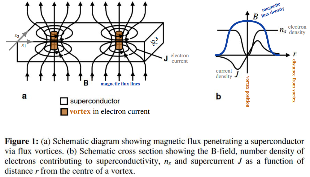
In this case the “sphere” through which the total magnetic flux density is measured is nominally the plane filled by the superconducting material, but since far away from any vortex the magentic flux has to vanish, this plane appears to the fluxes via its one-point compactification with the “point at infinity” adjoined.

These vortex strings are solitons in that the flux density is everywhere finite, and yet the “bumps” in the flux density are topologically stable. Much like a bump in a rug cannot be flattened as long as the boundary of the rug is fixed in place, so the requirement that flux densities “vanish at infinity” keeps the vortex strings in place — or at least this is the case once we take account of Dirac flux quantization below.

In summary:

The spacetime domains on which to exhibit fluxes of singular EM-branes (monopoles) and of solitonic EM-branes (vortices) are as shown on the left of the following graphics, respectively, whose right hand side already shows the classifying maps of their quantized charges, further discussed below:

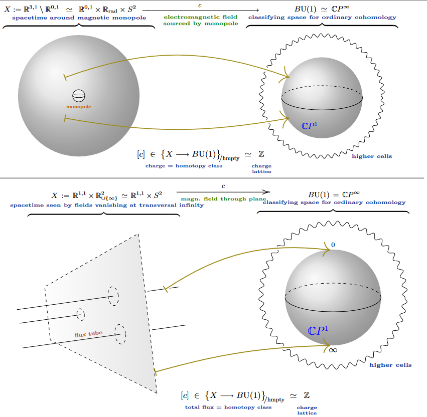
The fact that there are, generally, these two kinds of “branes imprinted on flux” is “well-known” and yet underappreciated:

Singular versus solitonic branes

Generally, imprinted on flux densities may be two kinds of branes, here to be called:

1. singular branes (black branes) reflected in diverging flux density at singular loci that are to be removed from spacetime,

   Beware that in supergravity these are also called “elementary branes” [Duff & Lu 1994], in reference to how black holes carry the same quantum numbers as elementary particles – but here we rather not conflate these two aspects.

2. solitonic branes reflected in finite flux density which is localized in that it vanishes at infinity, transversally.

   The terminology “solitonic brane” was introduced in Duff, Khuri & Lu 1992, 1994 and Duff & Lu 1993, 1994 to mean stable but non-singular brane-like solutions to (supergravity/flux) equations of motion (“solitons”).

This general distinction between singular branes and solitonic branes is important for the correct identification of the implications of choices of flux quantization-laws on the corresponding brane charges.

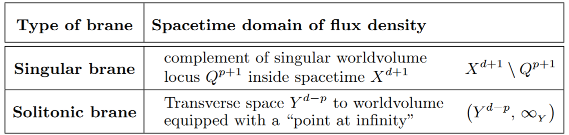
Spacetime domains for brane fluxes. More formally, one may encode these two cases by slightly adjusting the nature of the spacetime domain on which fluxes are actually defined [cf. SS23-MF, §2.1]:

1. fluxes sourced by singular branes of dimension $p+1$ inside spacetime $X^{d+1}$ are actually defined on the complement $X^{d+1} \setminus Q^{p+1}$ of their singular worldvolume,

2. fluxes sourced by solitonic branes of codimension $d-p$ are actually defined on their transverse space $T^{d-p}$ equipped with a “point at infinity” on which they are required to vanish.

The condition of flux densities vanishing at infinity on some space is naturally formalized by considering the larger category of pointed topological spaces $(X, x \in X)$ (we discuss further below how to properly speak of differential geometric smoothness in this context) and regarding their given “base point” as being the “point at infinity”, whence we shall write $(X, \infty_X)$ for the generic pointed space. Then a function “vanishing at infinity” on $(X,\infty_X)$ is a function on $X$ that literally vanishes at $\infty_X$.

For example:

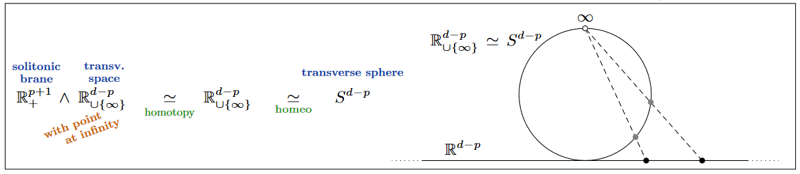
1. The result of adjoining to $\mathbb{R}^n$ its “point at infinity” (this is called its one-point compactification, here to be denoted $\mathbb{R}^n_{\cup \{\infty\}}$) is homeomorphic to the $n$-sphere with any basepoint:

   $$\mathbb{R}^n_{\cup \{\infty\}} \,\underset{homeo}{\simeq}\, S^n \,.$$

2. On the other hand, to consider unconstrained functions on some $X$ in this context, we may regard all the points of $X$ as being at finite distance by declaring that the “point at infinity” is disjoint from $X$, hence by considering the disjoint union (denoted “$\sqcup$” as opposed to “$\cup$”):

   $$X_{\sqcup \{\infty\}} \;\coloneqq\; X \sqcup \{ \infty \} \,.$$

Given two such pointed spaces, their smash product “$\wedge$” is their Cartesian product with all points that are at infinity in either factor identified with a single new point at infinity:

$$\big( X,\, \infty_X \big) \wedge \big( Y,\, \infty_Y \big) \;\; \coloneqq \;\; \frac{ X \times Y }{ X \times \{\infty_Y\} \,\cup\, \{\infty_X\} \times Y }$$

Example

(The case of flat branes.)
In the case of flat branes — i.e. with Cartesian worldvolumes inside Minkowski spacetime — both these spacetime domains are homotopy equivalent to spheres, but of different dimensions:

(1.) The spacetime domain for flat singular branes is homotopy-equivalent to the unit sphere in the transverse space, hence the sphere around the singular brane locus:

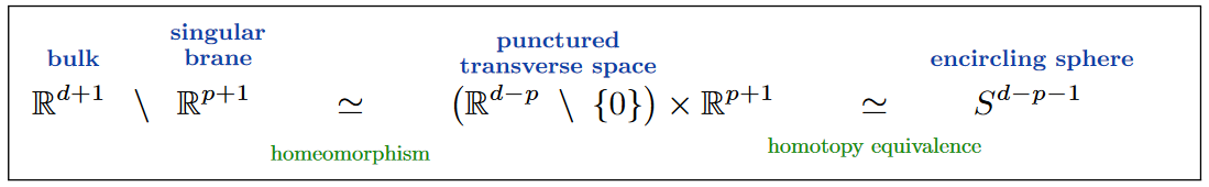
(2.) The spacetime domain for flat solitonic branes is homotopy equivalent to the sphere which is the one-point compactification of the transverse space (its stereographic projection):

Example

(the flat branes of electromagnetism)
Specifying Ex. to the case of ordinary electromagnetic flux (above) it follows from this general reasoning that a flux density 2-form $F_2$ in $D=3+1$ may reflect the presence of

1. singular 0-branes with spacetime domain

   $$\mathbb{R}^{3,1} \setminus \mathbb{R}^{0,1} \,\underset{\mathrm{homeo}}{\simeq}\, \mathbb{R}^{0,1} \times \mathbb{R}_{\gt 0} \times S^2 \,\underset{\mathrm{hmtp}}{\simeq}\, S^2$$

2. solitonic 1-branes with spacetime domain

   $$\mathbb{R}^{1,1}_+ \wedge \mathbb{R}^{2}_{\cup \{\infty\}} \;\underset{homeo}{\simeq}\; \mathbb{R}^{1,1}_+ \wedge S^2 \;\underset{hmtp}{\simeq}\; S^2$$

which are exactly the familiar cases of magnetic monopoles (hypothetical) and Abrikosov vortex strings (observed), discussed above.

Example

(near-horizon geometries of singular branes)
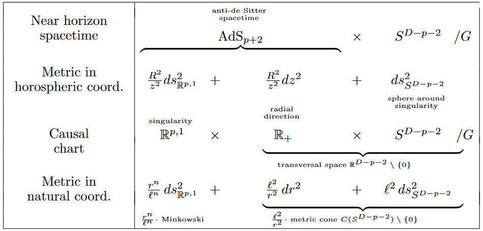
The idea of regarding singular branes from the complement of their singular locus in spacetime is familiar from the AdS/CFT correspondence:

The near horizon geometry of any $\gt 1/4$ BPS black brane are all product spaces of an anti de Sitter spacetime with a (free discrete quotient of) a sphere (a spherical space form) around the singularity [Acharya, Figueroa-O’Farrill, Hull & Spence 1999]. On a causal chart of AdS spacetime, this is homeomorphic to the flat brane complements from Ex. :

In general, the spacetime domain on which to measure flux densities may be a mix of these purely singular and purely solitonic situations, in which case the notions of singular and of solitonic branes blend into each other:

Example

(solitonic branes in KK-compactifications)

In mild generalization of Ex. , consider the case that spacetime is a trivial circle-fiber bundle over a Minkowski spacetime

$$X^D \,\equiv\, \mathbb{R}^{1,d-1} \times S^1 \,.$$

In this case the flux sourced by solitonic branes of codimension $n$ as seen on the base spacetime $\mathbb{R}^{1,d-1}$ is measured on the smash product space

$$\big( S^1 \times \mathbb{R}^n \big)_{\cup \{\infty\}} \;\underset{homeo}{\simeq}\; S^1_{\sqcup \{\infty\}} \wedge \mathbb{R}^n_{\cup \{\infty\}} \;\underset{homeo}{\simeq}\; S^1_{\sqcup \{\infty\}} \wedge S^n \,.$$

This was maybe first understood by Bergman, Gimon & Hořava 1999, §2.2 & §2.3 (there in slightly different language).

Higher fluxes and their brane sources

On this backdrop of ordinary electromagnetic flux (above) and of the general rule for measuring flux sourced by singular branes or solitonic branes (above) it clearly makes sense to consider physical theories of higher gauge fields whose precise nature remains to be discussed, but whose flux densities are reflected in higher-degree differential forms $F^{(i)}(X^D)$, these possibly being of different field species to be labeled by a finite index set $I \in FinSet$ and jointly to be denoted as follows:

(3)$$\vec F \;\equiv\; \Big\{ F^{(i)} \,\in\, \Omega_{dR}^{deg_i}\big( X^D \big) \Big\} \,.$$

(4)

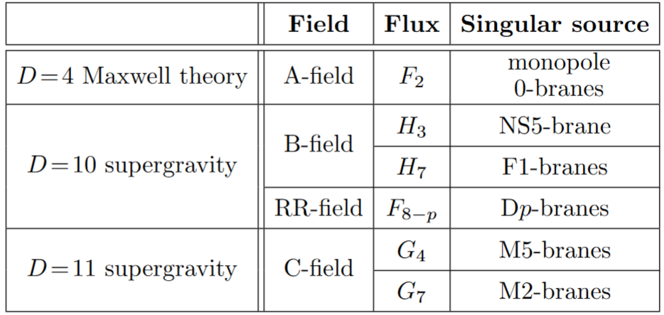
Remarkably, such higher flux densities “automatically” appear in higher dimensional supergravity, namely as “superpartners” of the gravitino-field that cannot be accounted for by the graviton itself. In particular in D=10 supergravity and D=11 supergravity these higher flux densities are known under the (now) fairly standard symbols shown on the right, along with the standard name of the correspoding singular branes (the “higher-dimensional monopoles”).

• D=10 supergravity: B-field$\leftrightarrow$NS5-brane/F1-brane and RR-field$\leftrightarrow$D-branes

• D=11 supergravity: C-field$\leftrightarrow$M5-brane/M2-brane.

(cf. Blumenhagen, Lüst & Theisen 2013, §18.5, Table 18.3)

Remark

(singular vs. solitonic D-branes)
Historically, the D-branes in D=10 supergravity were first identified as such [Polchinski 1995, cf. (14)] in their singular brane incarnation [Duff & Lu 1994], while their incarnation as solitonic branes (in the above sense) was considered only later in the context of the hypothesis of D-brane charge quantization in K-theory [Bergman, Gimon & Hořava 1999, §2.2 & §2.3, building on earlier discussion by Witten 1998, §4.1] to be discussed further below.

But beware that the distinction between these two aspects of D-branes, while “well-known”, is not commonly highlighted in the literature (not even in these original articles).

The above flux densities in 11d and 10d are closely related:

Example

(double dimensional reduction of fluxes form 11d to 10d)
Consider the case of C-field flux densities $G_4$ and $G_7$ on an 11-dimensional spacetime $X^{11}$ which is the total space of a circle-principal bundle

and denote by

• $\theta \,\in\, \Omega^1_{dR}(X^{11})$ any fiberwise Maurer-Cartan form along the fibers (i.e. an Ehresmann connection form),

• $F_2 \,\in\, \Omega^2_{dR}(X^{10})$ the corresponding (first) Chern class-characteristic form, i.e. the curvature form whose pullback to $X^{11}$ is

  $$\mathrm{d} \theta \;=\; p^\ast F_2 \,.$$

Assuming that all flux densities are $S^1$-inavariant (hence focusing on their 0th KK-modes) they decompose into a basic component (a differential form on $X^{10}$, pulled back along the projection $p$) and the wedge product of a basic differential form with the Maurer-Cartan form $\theta$ on the $S^1$-fibers:

(5)

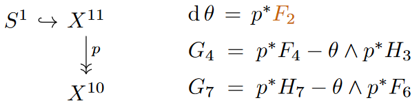
This is the process of “double dimensional reduction” – called this way since both spacetime dimension is reduced by Kaluza-Klein reduction on a fiber space, but also the degrees of densities of fluxes “through the fiber space” are decreased – known as part of the duality between M-theory and type IIA string theory: The new component flux densities $H_3$ and $H_7$ are interpreted as those of the B-field and the component flux densities $F_4$ and $F_6$ (and $F_2$) as those of the RR-field in type IIA supergravity.

Here the flux density $F_2$, which in 10d is understood as witnessing singular $D_6$-brane sources, is a $\color{orange}\text{gravitational}$ flux from the 11d point of view: If $X^{10} \,=\, \mathbb{R}^{6,1} \times \mathbb{R}_{\gt 0} \times S^2$ is the spacetime domain around a flat singular D6-brane (cf. above), then the total space of the circle-principal bundle $X^{11}$ (a multiple of the complex Hopf fibration) is known as the corresponding “KK-monopole” spacetime.

This transmutation, under Kaluza-Klein compactification, of parts of the gravitational field in higher dimensions into gauge fields in lower dimensions is a major subtlety in choosing flux quantization laws: Since these laws apply to higher gauge fields but not directly to the field of gravity, there may appear new possibilities for flux quantization after KK-reduction to lower dimensions which do not come from flux quantization in higher dimensions.

Equations of motion of higher flux

As we now turn to the equations of motion for flux densities (the analogs of Maxwell's equations for electromagnetic flux), the key move towards identifying possible flux quantization laws (below) is to arrange these equations, equivalently, as:

1. a purely cohomological system of differential equations known as higher Bianchi identities;

2. a purely geometric system of linear equations expressing a Hodge self-duality,

the point being that the first item is entirely “algebro-topological” (homotopy-theoretic), while dependency on geometry, namely on the spacetime metric (the field of gravity) is all isolated in the second item.

It turns out [SS23-FQ] that from such duality-symmetric laws of flux, the canonical phase space of the higher gauge theory, including the flux-quantization structure may be obtained straightforwardly, without going through the traditional and thorny route of BRST-BV analysis based on an stationary action principle given by a Lagrangian density.

This move of isolating “pre-metric flux equations” supplemented by a “constitutive” duality constraint has a curious status in the literature. On the one hand, it is elementary and immediate as an equivalent re-formulation of the usual form of (higher) Maxwell-type equations of motion, and as such has been highlighted a century ago [Kottler (1922a), (1922b), Cartan (1924) §80, Dantzig (1934)] and again more recently [Hehl & Obukhov (2003), Delphenich (2005a), (2005b)] (see the surveys Hehl, Itin & Obukhov 2016 and Delphenich (202x)).

While the broader community does not seem to have taken much note of “premetric electromagnetism” as such, we notice that just the same perspective is evidently what in supergravity and string theory is called “duality-symmetric” [Bandos, Berkovits & Sorokin 1998] or “democratic” [Mkrtchyan & Valach 2023] formulations of fluxes in supergravity (see Examples and below).

Definition

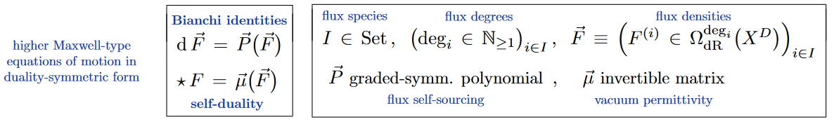
Higher Maxwell-type equations (in vacuum) on a tuple (3) of flux differential forms $\vec F \,\equiv\, \big\{F^{(i)}\big\}_{i \in I}$ of any degree $deg_i \geq 1$ on a $D$-dimensional spacetime $X^D$ (a pseudo-Riemannian manifold) of any dimension $D = d+1 \geq 2$ , is:

1. any system of polynomial $\vec P(-)$ first order exterior-differential equations $\mathrm{d} \vec F \,=\, \vec P\big(\vec F\big)$ (the higher Bianchi identities, crucially admitting polynomial “self-sourcing” of fluxes);

2. subject to a linear $\vec \mu(-)$ Hodge-self-duality relation $\star \vec F \,=\, \vec \mu\big(\vec F\big)$ (the “constitutive equation”):

(6)

Concretely:

• $\vec P$ is an $I$-tuple of graded-symmetric polynomials with rational coefficients in $I$ variables of degrees $\vec deg$,

• $\vec \mu$ is a linear endomorphism on the vector space spanned by these variables.

Remark

The equations in Def. imply that $\vec P$ and $\vec \mu$ respect degrees in a certain evident way. Moreover, the following property of the Hodge star operator on Lorentzian manifolds (see there) implies further constraints on the available higher Maxwell-type equations:

(7)$$\star \, \star \, F_{deg} \;\; = \;\; -(-1)^{deg(D-deg)} \, F_{deg} \,, \;\;\;\;\;\;\;\; \text{for} \; F_{deg} \,\in\, \Omega^{deg}_{dR}(X^D) \,.$$

This controls notably the existence of genuinely self-dual higher gauge theories, see Ex. below.

Remark

Not all higher gauge theories are of the higher Maxwell-form (Def. ): For instance higher Chern-Simons type theories are different.

Example

(Motion of the ordinary electromagnetic fluxes)

The classical Maxwell equations expressed in terms of differential forms (see basic references here) are as shown on the left, with their premetric form shown on the right (see the references there):

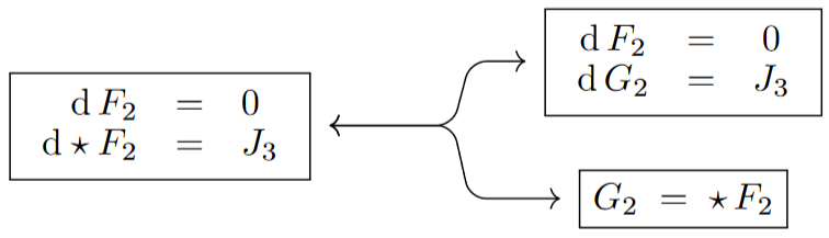
Here the differential 3-form $J_3$ embodies the density of an electric current carrying an electric field and inducing a magnetic field. This kind of background source term, where the source is not given by (a polynomial in) the flux densities themselves, does not fit into the Definition and shall be disregarded for the purpose of the present discussion, meaning that we focus on the special case of Maxwell’s equations “in vacuum”:

It is clear that, mathematically at least, Ex. , makes sense more generally for flux densities of any degree. In particular:

Example

(Motion of unbounded RR-field fluxes)

The equations of motion of the RR-field fluxes in D=10 supergravity in the case of vanishing B-field-fluxes are often taken to be as follows (e.g. Mkrtchyan & Valach 2023):

(8)

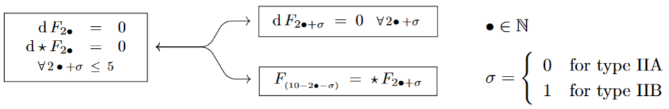
(While we may think of $\bullet$ as ranging over all natural numbers – which is suggestive in view of Hypothesis K discussed below – of course on the given spacetime manifold of dimension $D=10$ all differential forms of degree $\gt 10$ vanish identically.)

and, more generally, those with non-vanishing B-field as follows:

(9)

Beware, while these equations are now often stated in this form, and while this is the form that motivates the traditional Hypothesis K, it is at least subtle to see them in entirety as actually arising from ordinary D=10 supergravity (namely from KK-compactification of D=11 supergravity), since in that context:

1. The fluxes $F_0$ and $F_{10}$ are not actually present (they arise only in massive type IIA supergravity, which has its own subtleties).

2. The flux $H_7$ has a non-linear Bianchi identity ($\mathrm{d} H_7 \,=\, -F_4 \wedge F_4 + F_2 \wedge F_6$) which does not fit the suggestive pattern.

For more on this see Ex. below.

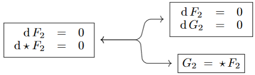
Notice that in type IIB, (8) describes a flux density ($F_5$) which is Hodge dual (not just to any other flux in the tuple but) to itself, $F_5 \,=\, \star\, F_5$. Generally we have:

Example

(Motion of self-dual higher gauge field fluxes)

Since Def. regards every higher gauge theory (of Maxwell-type) as being “self-dual” in a sense, the equations of motion of flux densities of actual self-dual higher gauge fields – in the strict sense that one and the same flux density form is required to be Hodge dual to itself – are readily an example of Def. :

(10)

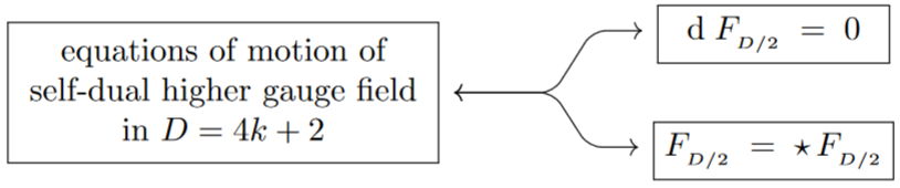
Due to the properties of the square of the Hodge operator (7), this has non-trivial solutions iff the degree of the flux is odd, $deg = 2k+1$, and hence iff spacetime dimension is $D = 4k + 2$, $k \in \mathbb{N}$.

What is much more clear-cut than the example of fluxes in D=10 supergravity (Ex. ) is the following example of fluxes in D=11 supergravity, where at least on flat spacetimes there is no ambiguity in the literature:

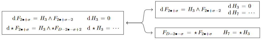
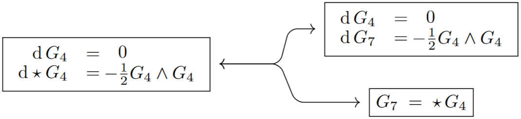
Example

(Motion of C-field fluxes)

The equations of motion of the C-field in D=11 supergravity (originally the “3-index A-field” due to Cremmer, Julia & Scherk 1978, see also D’Auria & Fré 1982, p. 131; Castellani, D’Auria & Fré 1991, §III.8; Miemiec & Schnakenburg 2006, p. 32) are traditionally as shown on the left here, with their equivalent “duality-symmetric” reformulation shown on the right (see the references there):

(11)

Example

(Motion of type IIA B&RR-field fluxes)

Under double dimensional reduction of the C-field flux from Ex. along a circle-bundle as in (5), the equations of motion (11) of the C-field from are equivalently expressed in terms of its B&RR-field-components as follows [Mathai & Sati 2004, §4; FSS17-Sph, §3; see also Figueroa-O’Farrill & Simón 2003, §1.2]:

(12)

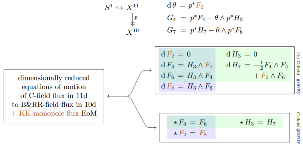
These are the equations of motion of the flux densities of type IIA supergravity in their duality-symmetric formulation [Cremmer, Julia, Lu & Pope 1998, §3].

Several terms in (12) deserve special attention, either for how they appear or for how they do not appear:

1. The Hodge dual $F_8 \,\coloneqq\, \star \, F_2$ is not part of the C-field in 11d, but is part of the gravitational field (the Hodge star encodes the 10d metric and $F_2$ is an aspect of the 11d fiber geometry). The expression for $\mathrm{d} H_8$ arises as part of the gravitational field equations [Cremmer, Julia, Lu & Pope 1998 (3.4)].

2. The presence in type IIA supergravity of the non-linear Bianchi identity for $H_7$, albeit readily verified and “well-known” at least since CJLP98 (3.4), is not as widely appreciated as the pattern (9) from Ex. – which it breaks.

3. No flux densities $F_0$ nor $F_{10}$ appear in 10d from KK-reduction on a circle, nor are they part of type IIA supergravity. These fluxes are instead part of massive type IIA supergravity whose relation to D=11 supergravity/M-theory remains less understood, see the references here.

Solution space of the flux equations

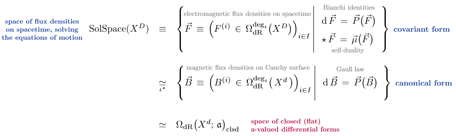
The phase space. Abstractly, the phase space of a any field theory is nothing but the space of all those field histories that satisfy the given equations of motion (the “on-shell” field histories). Phrased this way, this is sometimes called the covariant phase space, to emphasize that no choice of foliation of spacetime by Cauchy surfaces has been or needs to be made.

(13)

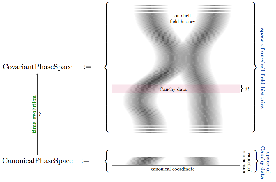
The more traditionally familiar canonical phase space (common physics jargon, somewhat incompatible with the mathematician’s “canonical”) is instead a parameterization of the covariant phase space by initial value data on a choice of Cauchy surface. This choice breaks the “manifest covariance” of the covariant phase space. Nevertheless, if a Cauchy surface exists at all (hence on globally hyperbolic spacetimes), then both these phase spaces are equivalent, by definition, the equivalence being the map that generates from initial value data the essentially unique on-shell field history that evolves from it (possibly up to gauge transformation).

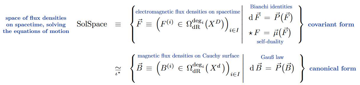
Solution space of on-shell flux densities. At this point in the discussion, the full gauge field content is not yet determined – this will only be implied by a choice of flux quantization below – so far we are only considering the flux densities of the would-be gauge fields. To remember this, we shall call the space of flux densities solving their equations of motion (Def. ) the solution space; and we are after its incarnation as a canonical solution space of initial value data on a Cauchy surface. But this goes a long way, since the higher Maxwell-type equations of motion constrain exclusively the flux densities: Once the flux-quantization the canonical phase will simply consist of all flux-quantized gauge potentials compatible with the flux densities in the canonical solution space.

Proposition

(SS23-FQ) On a globally hyperbolic spacetime $X^D \,\simeq\, \mathbb{R}^{0,1} \times X^d$, the solution space to given higher Maxwell-equations of motion (Def. ) is isomorphic to the solution of (just) the duality-symmetric Bianchi identities (6) restricted (pulled back to) to any Cauchy surface $\iota \,:\, X^d \hookrightarrow X^D$, there to be called the higher Gauß law:

(14)

Example

(Solution- and phase-space of ordinary electromagnetism)
In the case of ordinary vacuum electromagnetism, Prop. applied to the ordinary Maxwell equations from Ex. says that the initial value data on a Cauchy surface $X^3$ is given by independently specifying magnetic and electric flux densities

$$B,\, E \,\in\, \Omega^2_{dR}(X^3)$$

subject only to the ordinary Gauß laws:

$$\mathrm{d} B \,=\, 0 \,,\;\;\; \mathrm{d} E \,=\, 0 \,.$$

Indeed, the actual phase space of electromagnetism, after introducing a gauge potential, is well-known (see there) to have as

• canonical coordinate the gauge potential $A$,

• canonical momentum the electric flux density $E$.

Thereby $B \,\equiv\, curv\big(\widehat{A}\big)$ is indeed independent from $E$ (and satisfies its Gauß law definitionally, while the Gauß law on $E$ is a phase space constraint).

Notice how, thereby, this traditional split of initial value data into canonical coordinates and canonical momenta (whose definition requires assumption and variation of a Lagrangian density) is preempted here, under Prop. , already by the pregeometric/duality-symmetric formulation of Maxwell’s equations (in Ex. ), in the sense that the spacetime archetypes of the canonical coordinates and momenta on a Cauchy surface (the former seen under the differential) are just the ordinary flux density $F_2$ (since $B = \iota^\ast F_2$) and its “duality partner” $G_2$ (since $E = \iota^\ast G_2$).

Remark

(Gravity “decouples” on canonical phase space)
The inverse isomorphism (14) is given by time evolution of initial value data. Notice that the pseudo-Riemannian metric on $X^D$ – the background field of gravity – enters only in determining the nature of this isomorphism $\iota^\ast$ (the time evolution away from the Cauchy surface), but does not affect the nature of the initial value data (of the canonical phase space) as such.

It is this “decoupling” on the canonical phase space of the gravity/metric effects from the phase space Gauß law constraint which allows to gain plenty of insight into brane configurations from purely cohomological analysis of fluxes on Cauchy surfaces, disregarding the full solution of the coupled (super-)gravity equations of motion:

Qualitative solutions: Brane intersections

Prop. implies that on globally hyperbolic spacetimes the structure of on-shell flux densities in supergravity may be analyzed already by solving the (non-linear) Gauss law (14) for duality-symmetric fluxes on any Cauchy surface and ignoring the coupling to gravity there (assuming only that there exists at least one gravitational field configuration which solves its Einstein equations with source terms of this form). Since the same Gauss law also governs the admissible flux quantization laws below we showcase a couple of qualitative solutions to highlight just how much non-trivial (brane-)physics is encoded in these equations.

Example

(D6/D8-intersections and the Hanany-Witten effect) A popular conjecture by Hanany & Witten 1997 states that the expected $\mathrm{D}_{\!p}$-branes stretching between $\mathrm{NS}_5$ and $\mathrm{D}_{p+2}$ (cf. above) are “created” as the $\mathrm{D}_{\!p+2}$-branes are “dragged over” the $\mathrm{NS}_5$, intuitively like a pole will cause a spike in a rubber sheet that is pulled over its tip. It was suggested by Marolf 2001 (§2) that this Hanany-Witten effect should be understandable entirely from analysis of the flux Bianchi identities (14).

For the case of NS5/D6/D8-brane intersections [e.g. Hanany & Zaffaroni 1998 (§2.4); Bergshoeff, Lozano & Ortin 1998 (p. 60) this may be seen as follows (the other cases work analogously):

Here, by the flux equation (9)

(15)$$\begin{array}{l} \mathrm{d} F_0 \;=\; 0 \,, \\ \mathrm{d} \, F_2 \;=\; H_3 \wedge F_0 \,, \end{array}$$

the flux density $F_0$ of $\mathrm{D}_8$-branes (the “Romans mass”) is a locally constant function that vanishes in the vacuum and jumps by $N$ units across the singular locus of $N$ $\mathrm{D}_8$-branes (cf. e.g. Fazzi 2017 (p. 40)). But this means that:

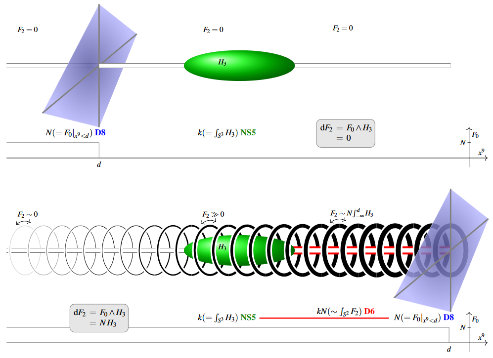
(1.) When the $\mathrm{NS}_5$-brane is located in the vacuum where $F_0 = 0$, then its sourcing of $F_{2}$-flux is “switched off” by the vanishing $F_0$-factor in (15), hence if $F_2$ vanishes at infinity then the PDE demands it vanishes everywhere, reflecting the absence of $\mathrm{D}_6$-branes.

(2.) When the $\mathrm{NS}_5$-brane is located on the other side of the $\mathrm{D}_8$-branes, where $F_0 = N$, then the equation (15) shows that $F_2$-flux/$\mathrm{D}_6$-number density which vanishes far away will increase along the coordinate axis $x^9$ orthogonal to the $\mathrm{D}_8$-branes in proportionality to the $\mathrm{d}x^9$-component of the flux $H_3$, and hence pronouncedly so as one crosses the $\mathrm{NS}_5$-brane locus.

Example

(M2$\perp$M5-brane intersections on “M-strings”)
Consider the singular loci of two parallel flat M5-branes at a distance $2d \gt 0$

each reflected by unit 4-flux through their surrounding 4-spheres:

$$G_4^{{}^{(i)}} \;\coloneqq\; \mathrm{dvol}_{S^4} \,\in\, \Omega^4_{\mathrm{dR}}(S^4) \xhookrightarrow{ \quad \mathrm{pr}_{S^4}^\ast \quad} \Omega^4_{\mathrm{dR}}\Big( \mathbb{R}^{1,5}_{{}_{(i)}} \times \mathbb{R}_{\plus} \times S^4 \Big) \;\simeq\; \Omega^4_{\mathrm{dR}}\Big( \mathbb{R}^{1,10} \setminus \mathbb{R}^{1,5}_{{}_{(i)}} \Big) \,.$$

With the total 4-flux thus $G_4 \;\coloneqq\; G_4^{(1)} + G_4^{(2)} \,,$ the C-field Bianchi identity (Ex. ) says that the flux $G_7$ sourced by M2-branes obeys the equation

(16)$$\begin{array}{rcl} \mathrm{d} G_7 &=& - \tfrac{1}{2} G_4 \wedge G_4 \\ &=& - G_4^{(1)} \wedge G_4^{(2)} \,, \end{array}$$

where the wedge product of the two translated $S^4$-volume forms acts as an effective “electric potential” source term.

For the purpose of illustration we consider a qualitative sketch of the 2-dimensional analog of this situation, where the 4-forms are replaced by 2-forms:

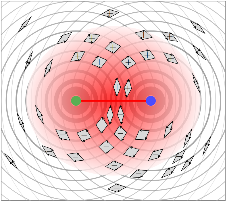
Effective dipole of quadratic brane flux. The figure means to indicate the nature of the differential 2-form which is the wedge product of two copies of the pullback of $\mathrm{dvol}_{S^1}$ to around either of the punctures (the brane loci) in the 2-punctured plane. Here:

• the strength of the circular lines indicates the absolute value of the flux density sourced by the respective 5-brane,

• the arrows indicate the orientation of the flux density of either 5-brane,

• the parallelograms indicate the orientation of their wedge product.

Evidently, the absolute value of the wedge product is concentrated near the 5-branes and particularly between them…

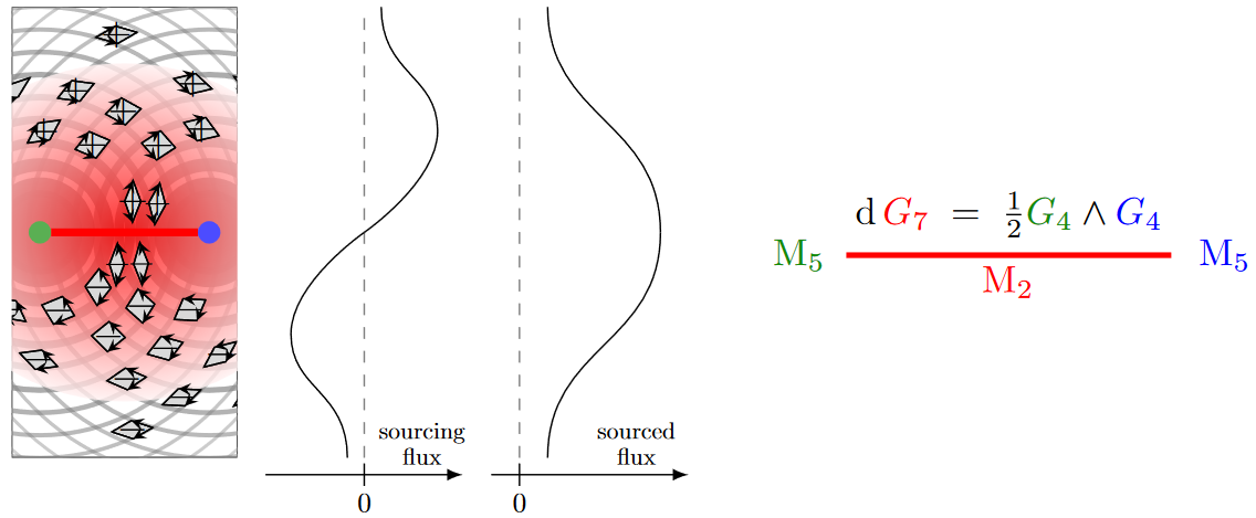
…but the orientation of the wedge product changes sign across the axis connecting the branes, as shown. This means that the flux sourced by this wedge product, according to (16), is, if vanishing at infinity, concentrated between the branes.

This sourced flux concentration (indicated in red) witnesses an M2-brane stretching between the two M5-branes. The intersection is known as the M-string.

Notice how in these examples we chose integral values for the total source brane fluxes. Next we discuss how such flux quantization is systematically enforced in the higher gauge theory.

Flux/Charge quantization laws

With the solution space (Prop. ) of higher Maxwell-type equations of motion (Def. ) in hand, the question of flux quantization is to further constrain the flux densities such that the total fluxes and their total source charges take values in some discrete space.

The technical issue to be resolved here is that:

• this is a global condition on the flux densities: The local flux densities may take any value (compatible with the equations of motion) and yet the total accumulation of all these local contributions needs to be constrained;

• the evident idea of constraining the ordinary integrals of the flux densities (their “periods”) makes sense only for closed differential forms and hence does not work for non-linear Bianchi identities (such as those of the C-field, Ex. , and the B&RR-field, Ex. ).

To resolve this, one may first observe that:

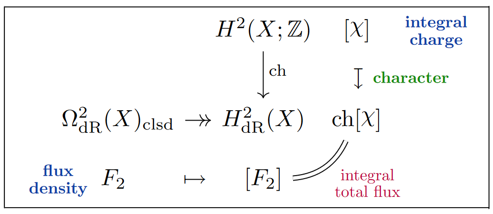
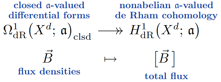
• the integrals/periods of ordinary closed differential $n$-forms $F_n$ over $n$-manifolds are in natural correspondence with their de Rham-classes, $[F_n] \in H^n_{dR}(-)$, which in turn are equivalently their “deformation classes”, namely their concordance classes: $H^n_{dR}(-) \,\simeq\, \Omega^n_{dR}(-)_{clsd}\big/_{cncrdnc}$,

• so that integrality of closed flux density $F_n$ is witnessed by an integral cohomology class $[\chi] \in H^n(X;\mathbb{Z})$ whose “de Rham character” image $ch[\chi] \in H^n_{dR}(X)$ coincides with the deformation class $[F_n]$

and then that this perspective generalizes [FSS23-Char, SS23-FQ]:

(1) Higher Maxwell-type equations (6) have a characteristic $L_\infty$-algebra $\mathfrak{a}$: The flux densities are equivalently $\mathfrak{a}$-valued differential forms, and the Gauss law (14) is equivalently the condition that these be closed (i.e.: flat, aka a “Maurer-Cartan element”; in Italian SuGra literature: “satisfying an FDA”).
(2.) Also (homotopy types (37) of) topological spaces $\mathcal{A}$ (under mild conditions) have a characteristic $L_\infty$-algebra: Their $\mathbb{R}$-rational Whitehead bracket $L_\infty$-algebra.
(3.) The nonabelian Chern-Dold character map turns $\mathcal{A}$-valued maps into closed $\mathfrak{l}\mathcal{A}$-valued differential forms, generalizing the Chern character for $\mathcal{A} =$ $\mathrm{KU}_0$.
(4.) The possible flux quantization laws for a higher gauge field are those spaces $\mathcal{A}$ whose Whitehead $L_\infty$-algebra is the characteristic one.
(5.) Given a flux quantization law $\mathcal{A}$, the corresponding gauge potentials are deformations of the flux densities into characters of a $\mathcal{A}$-valued map, witnessing the flux densities as reflecting discrete charges quantized in $\mathcal{A}$-cohomology.
(It is not obvious that this reduces to the usual notion of gauge potentials, but it does.)
(6.) These non-perturbatively completed higher gauge fields form a smooth higher groupoid: the “canonical differential $\mathcal{A}$-cohomology moduli stack”. Since these are now the flux-quantized on-shell fields, this is the phase space of the flux-quantized higher gauge theory.

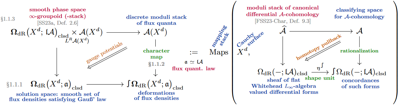
This flux-quantized phase space hence subsumes the “solitonic” fields with non-trivial charge sectors $\chi$, and as such is a non-perturbative completion of the traditional phase spaces (which correspond to a fixed charge sector only, typically to $\chi = 0$).

Incidentally, it follows (as discussed below) that the choice of flux quantization law $\mathcal{A}$ not only defines the solitonic content of the theory but completely characterizes it:

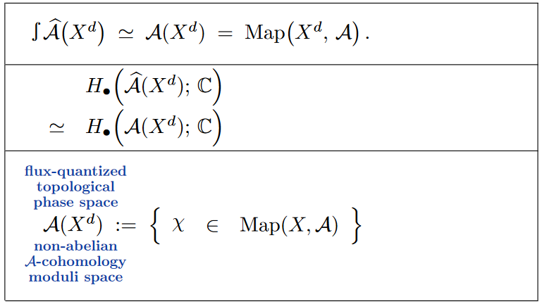
The shape (topological realization) of this phase space stack is the space of topological fields,

which implies that the ordinary homology of the phase space stack constitutes the topological quantum observables on the higher gauge theory.

Hence if one focuses only on the solitonic or topological field-content of the phase space, then we see plain $\mathcal{A}$-cohomology moduli of the Cauchy surface, with the full phase space stack serving to justify this object.

We now explain all this in more detail:

Total flux as Non-abelian de Rham cohomology

We explain how higher Bianchi identities (6) and their corresponding higher Gauss laws (14) are equivalently the closure (flatness) condition on differential forms valued in a characteristic $L_\infty$-algebra (Prop. below), so that total flux is a class in $\mathfrak{a}$-valued nonabelian de Rham cohomology (Def. below).

The notion of $L_\infty$- or strong homotopy Lie algebra is finally becoming more widely appreciated in physics, where they appear in various guises (see the references there). Here we are concerned with $L_\infty$-algebras which are (i) nilpotent, (ii) connective (iii) of finite type, in their joint incarnation as higher flux density coefficients and as higher Whitehead brackets (all to be explained in a moment), which one might refer to as the

Flux Homotopy Lie algebra triality.

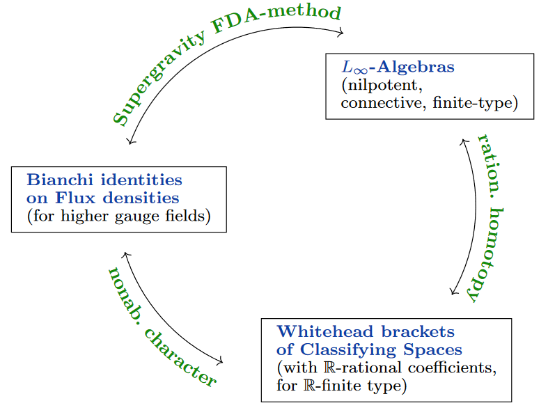
$\bullet$ With rational homotopy we are referring here specifically the fundamental theorem of dg-algebraic rational homotopy theory, mainly due to Quillen, Sullivan and Bousfield & Gugenheim, as reviewed in FSS23-Char, §5,

$\bullet$ by the FDA method in supregravity we are referring, with some hindsight, to the observations of van Nieuwenhuizen 1983; D Auria & Fré 1982; Castellani, D’Auria & Fré, as explained in FSS13, FSS18,HSS19, reviewed in FSS19-$\mathbb{Q}$Struc.

$\bullet$ The nonabelian character is the generalization of the Chern-Dold character map from topological K-theory and Whitehead-generalized cohomology to generalized non-abelian cohomology, constructed in FSS23-Char.

In particular, this means that $L_\infty$-algebras as used here are not directly to be understood as generalizations of the gauge Lie algebras familiar from Yang-Mills theory, which are coefficients of the gauge potentials, but instead as the coefficients of their flux densities (cf. Rem. ).

$L_\infty$-Algebras. Since we are assuming $L_\infty$-algebras to be connective and of finite type (meaning that they are degreewise finite-dimensional and concentrated in non-negative degrees) we may define them through their Chevalley-Eilenberg (CE) algebras in the following manner, which is not only convenient for dealing with the otherwise intricate sign rules, but also essential to their alternative perspectives in the above triality:

$\;\;$Chevalley-Eilenberg algebras of Lie algebras. Namely, for $\mathfrak{g}$ a finite-dimensional Lie algebra (our ground field is the real numbers, throughout) with Lie bracket a skew-symmetric linear map $[-,-] \,:\, \mathfrak{g} \otimes \mathfrak{g} \to \mathfrak{g}$, its linear dual vector space $\mathfrak{g}^\ast$ is equipped with the dual bracket $[-,-]^\ast \,:\,\mathfrak{g}^\ast \to \mathfrak{g}^\ast \wedge \mathfrak{g}^\ast$ which extends uniquely to a degree=1 derivation on the graded Grassmann algebra $\wedge^\bullet \mathfrak{g} \,:=\, \underset{n \in \mathbb{N}}{\bigoplus} \,\underbrace{\mathfrak{g}^\ast \wedge \cdots \wedge \mathfrak{g}^\ast}_{n\;factors}$:

(17)

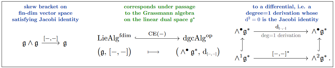
One readily checks that this derivation squares to zero iff the bracket satisfies its Jacobi identity(!):

$$\text{ Jacobi identity for } \; [-,-] \;\;\;\;\;\;\;\; \Leftrightarrow \;\;\;\;\;\;\;\; \mathrm{d}_{{}_{[-,-]}} \circ \mathrm{d}_{{}_{[-,-]}} \;=\; 0 \,.$$

The resulting differential graded-commutative (dgc) algebra $(\wedge^\bullet \mathfrak{g}^\ast, \mathrm{d}_{[-,-]})$ is known as the Chevalley-Eilenberg complex $\mathrm{CE}(\mathfrak{g})$ whose cochain cohomology computes the Lie algebra cohomology of $\mathfrak{g}$ (with trivial coefficients) — but the key point at the moment is that its construction is a fully faithful embedding the category of finite-dimensional Lie algebras into the opposite of that of dgc-algebras.

$\;\;$$L_\infty$-algebras of finite type. With ordinary Lie algebras viewed as special dgc-algebras this way, it is immediate to generalize them to the case where $\mathfrak{g}$ may be a graded vector space of degreewise finite dimension (“of finite type”): Namely, writing

$$(\mathfrak{g}^\vee)_n \;\coloneqq\; (\mathfrak{g}_n)^\ast, \;\;\;\;\;\;\;\;\;\;\;\; \wedge^\bullet \mathfrak{g}^\vee \;\coloneqq\; \mathrm{Sym}(\mathfrak{g}^\vee[1])$$

we can use verbatim the same construction:

A degree=1 derivation on $\wedge^\bullet\mathfrak{g}^\vee$ is determined by its restriction to $\wedge^1 \mathfrak{g}^\vee$, where it is a sum of co-$n$-ary linear maps, whose linear duals are identified as $n$-ary degree=(-1) brackets on $\mathfrak{g}[1]$:

(18)

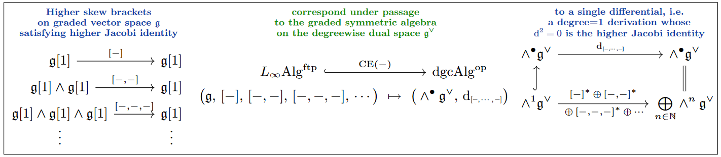
Here the simple condition that $\mathrm{d}_{{}_{[\cdots]}}$ be a differential implies a tower of conditions on these brackets, generalizing the Jacobi identity on an ordinary Lie algebra and known as the conditions that make $\big( \mathfrak{g}, [-], [-,-], [-,-,-], \cdots \big)$ an $L_\infty$-algebra:

$$\array{ \text{higher Jacobi identity for} \\ [-], [-,-], [-,-,-], \cdots } \;\;\;\;\;\;\;\;\; \Leftrightarrow \;\;\;\;\;\;\;\;\; \mathrm{d}_{{}_{[\cdots]}} \circ \mathrm{d}_{{}_{[\cdots]}} \;=\; 0 \,.$$

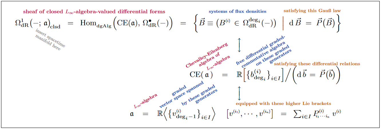
In other words, we may identify $L_\infty$-algebras of finite type as the formal dual to dgc-algebras whose underlying graded-commutative algebra is free on a graded vector space.

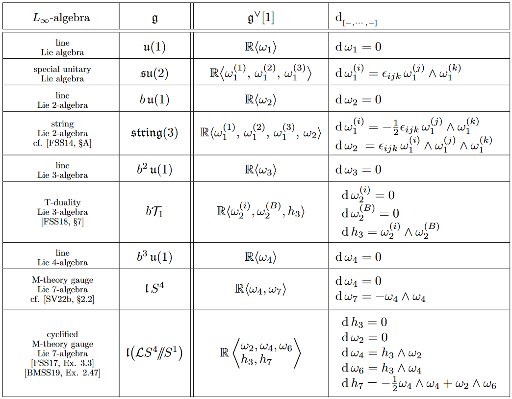
Some examples:

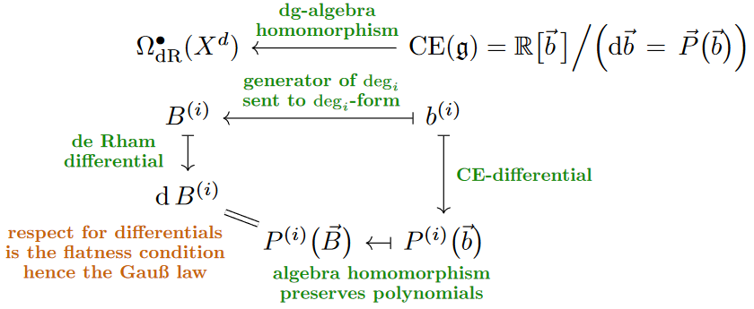
$\;\;$Flat $L_\infty$-algebra valued differential forms now have an immediate definition from this perspective: They are the dg-algebra homomorphism from their CE-algebras into de Rham algebras (aka “Maurer-Cartan elements”):

(19)$$\left. \begin{array}{l} \mathfrak{a} \in L_\infty Alg^{ftp} \\ X \in SmthMfd \end{array} \right\} \;\;\;\;\;\;\; \vdash \;\;\;\;\;\;\; \Omega^1_{dR}(X;\mathfrak{a})_{clsd} \;\coloneqq\; Hom_{dgAlg}\big( CE(\mathfrak{a}) ,\, \Omega^\bullet_{dR}(X) \big) \,.$$

Namely, a graded algebra homomorphism from a CE-algebra sends the algebra generators $\vec b$ to differential forms $\vec B$, and its respect for the differentials imposes on these differential forms exactly the closure/flatness condition:

Some examples:

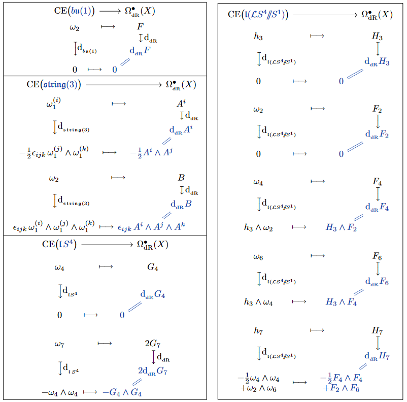
$\;\;$Flux densities satisfying Bianchi/Gauss laws are flat $L_\infty$-algebra-valued differential forms. Remarkably, it follows that polynomials $\vec P$ defining Bianchi identities (6) and Gauss laws (14) are equivalently structure constants of $L_\infty$-algebras $\mathfrak{a}$, such that the Bianchi/Gauss law is the closure/flatness condition on $\mathfrak{a}$-valued forms:

With Prop. this means:

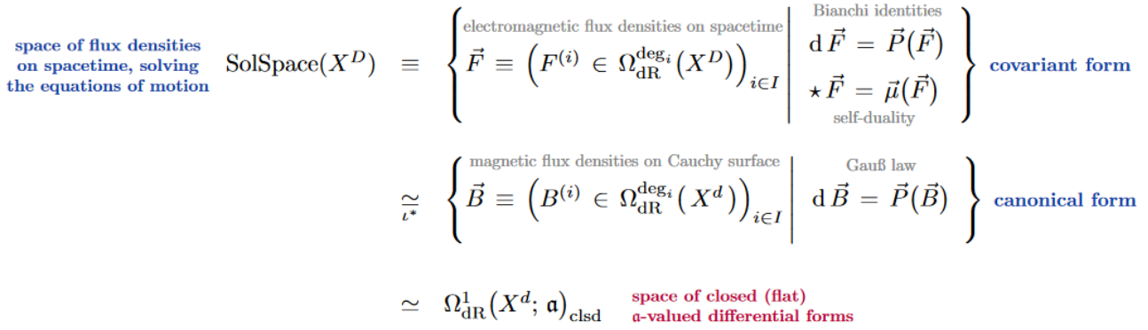
Proposition

Given a higher gauge theory of Maxwell-type (Def. ) with Bianchi identities given by graded-symmetric polynomials $\vec P$ (6) its space of flux densities solving the higher Maxwell equations is identified with the space of closed differential forms with coefficients in the $L_\infty$-algebra $\mathfrak{a}$ on $I$ $(\vec deg-1)$-graded generators with structure constants $\vec P$:

Example

The characteristic $L_\infty$-algebra of ordinary vacuum electromagnetism is the direct sum $b \mathfrak{u}(1) \oplus b \mathfrak{u}(1)$ of two copies of the line Lie 2-algebra, which by the previous example and Prop. corresponds to:

$$SolSpace_{EM}(X^3) \;\simeq\; \Omega^1_{dR}\big( X^3 ;\, b\mathfrak{u}(1) \times b\mathfrak{u}(1) \big)_{clsd} \;\simeq\; \Omega^2_{dR}(X^3) \times \Omega^2_{dR}(X^3) \,.$$

An element here is a pair $(B,E)$, where

1. the magnetic flux density is the curvature $B = \mathrm{curv}\big(\widehat A\big)$ of the gauge potential which plays the role of the “canonical coordinate” on the field space;

2. the electric flux density $E$ serves as the canonical momentum.

$\;\;$Total flux in non-abelian de Rham cohomology. While, with Prop. , the Gauss law of the given higher gauge theory of Maxwell-type constrains the flux densities on any Cauchy surface $X^d \hookrightarrow X^D$ to constitute a flat $L_\infty$-algebra valued differential form, the actual value of these differential forms depends on the Cauchy surface, which is an arbirary choice.

We should, therefore, regard as the total flux that aspect of the flux densities which is invariant under choice of Cauchy surfaces.

But since the Gauss law is (by Prop. ) nothing but the restriction to the Cauchy surface of the Bianchi identities (on the duality-symmetric flux densities of Def. ), the argument of Prop. shows that this invariant aspect is the equivalence classes of flux densities under concordance:

(20)

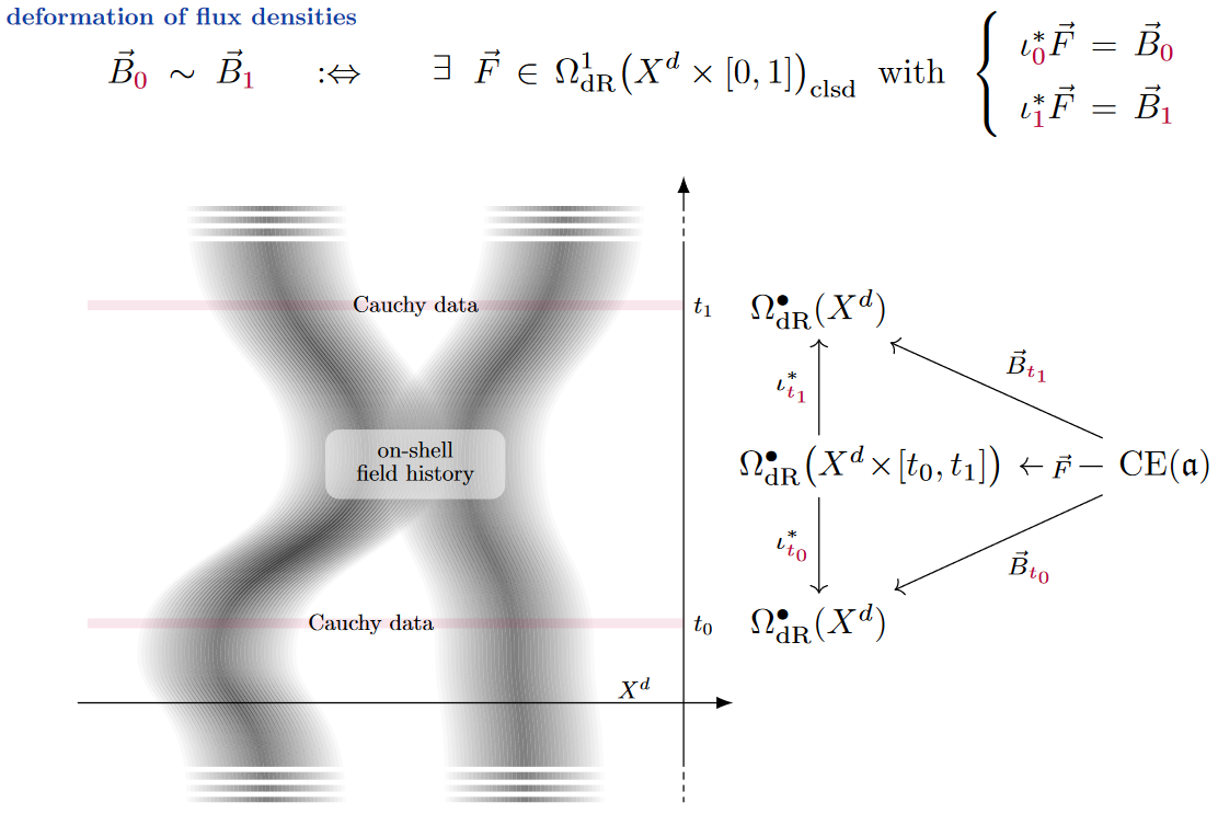
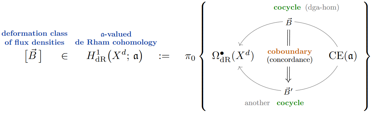
Definition

(non-abelian de Rham cohomology [FSS23-Char, Def. 6.3])
Given an $L_\infty$-algebra $\mathfrak{a}$ and a smooth manifold $X^d$, we say that a pair of closed $\mathfrak{a}$-valued differential forms $\vec B_0, \vec B_1 \,\in\, \Omega^1_{dR}\big(X^d;\mathfrak{a}\big)_{clsd}$ (19) are cohomologous iff they are concordant: iff there exists a closed $\mathfrak{a}$-valued differential form $\vec F$ on the cylinder over $X^d$ whose restriction (pullback) to the $k$th boundary component equals $\vec B_k$:

$$\vec B_0 \;\sim\; \vec B_1 \;\;\;\;\;\; \Leftrightarrow \;\;\;\;\;\; \exists \;\; \vec F \,\in\, \Omega^1_{dR}\big( X^d \times [0,1] ;\, \mathfrak{a} \big)_{clsd} \;\;\; \text{with} \;\;\; \left\{ \begin{array}{l} \vec B_1 \,=\, \iota_1^\ast \vec F \\ \vec B_0 \,=\, \iota_0^\ast \vec F \end{array} \right. \,.$$

The quotient set by this equivalence relation is $\mathfrak{a}$-valued nonabelian de Rham cohomology of $X^d$:

$$H^1_{dR}\big( X^d;\mathfrak{a} \big) \;\coloneqq\; \Omega^1_{dR}\big( X^d ;\, \mathfrak{a} \big)_{clsd} \Big/ \! \sim \,.$$

Remark

(flux conservation)

Regarding the image of flux densities in non-abelian de Rham cohomology as expressing their total flux it follows immediately that:

$\;\;\;\;\;$Total flux is conserved under time evolution.

Remark

(nonabelian de Rham cohomology as dg-homotopy classes)
For comparison to the flux quantization rules discussed below it is useful to understand this equivalently [FSS23-Char, Thm. 6.5] as the set of dg-homotopy classes of the corresponding dgc-homomorphisms:

Example

(FSS23-Char, Prop. 6.4)
In the case of ordinary electromagnetism and abelian higher gauge fields, hence for $\mathfrak{a} = b^n \mathfrak{u}(1)$ the line Lie $(n+1)$-algebra, Def. reduces to the ordinary notions:

1. $\Omega^1_{dR}\big(X^d; b^n\mathbb{R}\big)_{clsd} \,\simeq\, \Omega^{n+1}(X^d)_{clsd}$ are ordinary closed differential forms;

2. concordance between these is the coboundary relation in the ordinary de Rham complex;

3. $H^1_{dR}\big(X^d;\, b^n \mathbb{R}\big) \,\simeq\, H^{n+1}_{dR}\big(X^d\big)$ is ordinary de Rham cohomology.

and since the latter also gives the periods of closed differential forms, this recovers indeed the usual notion of total (integrated) flux.

Concretely, with

$$F_2 \;\coloneqq\; q \mathrm{dvol}_{S^2} \;\in\; \Omega^2_{dR}\big(S^2\big) \;\overset{p^\ast_{S^2}}{\longrightarrow}\; \Omega^2_{dR}\big(\mathbb{R}^3 \setminus \{0\}\big) \;\simeq\; \Omega^1_{dR}\big(\mathbb{R}^3 \setminus \{0\} ;\, b\mathbb{R} \big)$$

the flux density around a magnetic monopole of charge $q$ (1), the total flux is

$$\array{ H^2_{dR}\big( \mathbb{R}^3 \setminus \{0\} \big) &\simeq& H^2_{dR}\big( S^2 \big) &\simeq& \mathbb{R} \\ F_2 &\mapsto& \big[ F_2\, \big] &\mapsto& \int_{S^2} F_2 \mathrlap{ = q \,. } }$$

With on-shell flux densities thus understood as cocycles in nonabelian de Rham cohomology, we find their flux quantization laws among the corresponding torsion-ful nonabelian cohomology-theories:

Flux quantization laws as Nonabelian cohomology

We explain how the $\mathfrak{a}$-valued nonabelian de Rham cohomology of the previous subsection receives character maps from generalized nonabelian cohomology theories whose classifying spaces $\mathcal{A}$ have compatible rational Whitehead $L_\infty$-algebra $\mathfrak{l}\mathcal{A} \simeq \mathfrak{a}$ — whence $\mathcal{A}$ encodes a flux quantization law for Bianchi identities characterized by $\mathfrak{a}$, and lifting through the $\mathcal{A}$-character map corresponds to choices of charge quanta which source given total flux.

Classifying spaces for generalized cohomology. It is a classical fact of algebraic topology – which may have remained somewhat underappreciated in mathematical physics – that reasonable generalized cohomology theories have classifying spaces $\mathcal{A}$, in that the sets of cohomology classes assigned to a given domain space (which we take to be a smooth manifold $X$) are in natural bijection with the homotopy classes $\pi_0 Maps\big(-, \mathcal{A}\big)$ of continuous maps from $X$ into $\mathcal{A}$ (it is only the homotopy type (37) of $\mathcal{A}$ that matters here).

The archetypical examples are Eilenberg-MacLane spaces like $K(\mathbb{Z},n)$ which classify ordinary cohomology such as integral cohomology, in any degree $n$. As $n$ ranges, these EM-spaces happen to be loop spaces of each other, $K(\mathbb{Z},n) \simeq \Omega K(\mathbb{Z}, n+1)$.

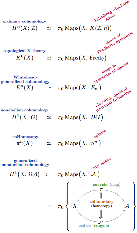
Generalizing from this classical example, one considers Whitehead-generalized cohomology theories which are classified by any sequences of pointed topological spaces $\{E_n\}_{n \in \mathbb{N}}$ equipped with weak homotopy equivalences $E_n \simeq \Omega E_{n+1}$, called a spectrum of spaces.

This implies that each $E_n$ is an infinite-loop space, which makes them be “abelian $\infty$-groups” reflecting the fact that the homotopy classes of maps into these spaces indeed have the structure of abelian groups.

The maybe most familiar example of such abelian generalized cohomology is topological K-theory, whose classifying space $KU_0$ may be identified with the space of Fredholm operators on an infinite-dimensional separable complex Hilbert space.

While Whitehead-generalized cohomology theory has received so much attention that it is now widely understood as the default or even the exclusive meaning of “generalized cohomology”, historically long preceding it is the nonabelian cohomology of Chern-Weil theory, classified by the original classifying spaces $B G$ of compact Lie groups $G$.

Unless $G$ happens to be abelian itself, this nonabelian cohomology does not assign abelian cohomology groups, nor even any groups at all, but just pointed cohomology sets. Nevertheless, as the historical name “nonabelian cohomology” clearly indicates, these systems of cohomology sets may usefully be regarded as constituting a kind of cohomology theory, too.

In this vein one may observe [FSS23-Char, §2] that (the homotopy type of) every connected space $\mathcal{A}$ is equivalently the classifying space of an infinity-group $\Omega \mathcal{A}$, namely of its own loop space regarded as an $A_\infty$-space under concatenation of loops), so that homotopy classes of maps into any connected space are examples of an evident generalization of Chern-Weil-style nonabelian cohomology.

A fundamental and historical example of such “truly-generalized” nonabelian cohomology is CoHomotopy, whose classifying spaces are the (homotopy types) of spheres.

Notice that “generalized nonabelian cohomology” is really “not necessarily abelian”: It subsumes all the other cases: For $E_\bullet$ a spectrum we have

$$E^n(X) \,\simeq\, H^1\big(X;\, \Omega E_n\big) \,.$$

Character maps on generalized cohomology. Moreover, it is classical that, over smooth manifolds, reasonable cohomology theories have their non-torsion content reflected in de Rham cohomology via character maps:

• on integral cohomology this is de Rham theorem,

• on ordinary non-abelian cohomology this is the Chern-Weil homomorphism,

• on topological K-theory this is the Chern character,

• on any Whitehead-generalized cohomology this is the Chern-Dold character

(21)

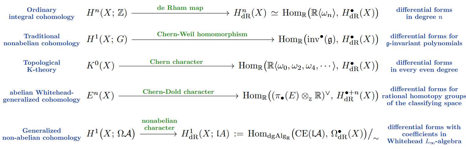
The nonabelian character in the generality of generalized non-abelian cohomology, such as CoHomotopy, is due to [FSS23-Char, Def. IV.2], constructed via the fundamental theorem of dg-algebraic rational homotopy theory. We next survey how this works.

The key point is that rational homotopy theory characterizes the non-torsion content of (the homotopy type of) a (classifying) space by an $L_\infty$-algebra-approximation $\mathfrak{l}\mathcal{A}$ to its loop space $\infty$-group $\Omega \mathcal{A}$.

Proposition

(Quillen-Sullivan-Whitehead $L_\infty$-algebra [cf. FSS23-Char, Prop. 4.23, 5.6 & 5.13])

For a topological space $\mathcal{A}$ which is

1. simply connected: $\pi_0(\mathcal{A}) = \ast$ and $\pi_1(\mathcal{A}) = 1$;

2. of rational finite type: $\mathrm{dim}_{\mathbb{Q}}\big(H^n(\mathcal{A}; \mathbb{Q})\big) \lt \infty$;

there is a polynomial dgc-algebra over $\mathbb{R}$, unique up to dga-isomorphism, whose

• generators are the $\mathbb{R}$-rational homotopy groups of $\mathcal{A}$,

  $$\mathrm{CE}(\mathfrak{l}\mathcal{A}) \;=\; \Big( \wedge^\bullet \big( \,{ \color{darkblue} \pi_\bullet \big( \Omega \mathcal{A} \big) \!\otimes_{{}_\mathbb{Z}}\! \mathbb{R} }\, \big)^\vee ,\, \mathrm{d}_{CE(\mathfrak{l}\mathcal{A})} \Big)$$

• cochain cohomology is the ordinary real cohomology of $\mathcal{A}$.

  $$H^\bullet\big( \mathrm{CE}(\mathfrak{l}\mathcal{A}) \big) = H^\bullet(\mathcal{A};\, \mathbb{R}) \,.$$

This dgc-algebra is known as the minimal Sullivan model of $\mathcal{A}$. By (18) it is the Chevalley-Eilenberg algebra of an $L_\infinity$-algebra which we denote by $\mathfrak{l}\mathcal{A}$ (essentially the “Quillen model”): The Whitehead bracket algebra structure on the $\mathbb{R}$-rational homotopy groups of the loop space

(22)$$\mathfrak{l}\mathcal{A} \;=\; \color{darkblue} \pi_\bullet\big( \Omega \mathcal{A} \big) \otimes_{\mathbb{Z}} \mathbb{R} \,.$$

(Think of “$\mathfrak{l}(-)$” as standing for “Lie” or for “loops”.)

Some examples for how to use Prop. to compute Sullivan models and hence $\mathbb{R}$-Whitehead $L_\infty$-algebras $\mathfrak{l}\mathcal{A}$ of spaces:

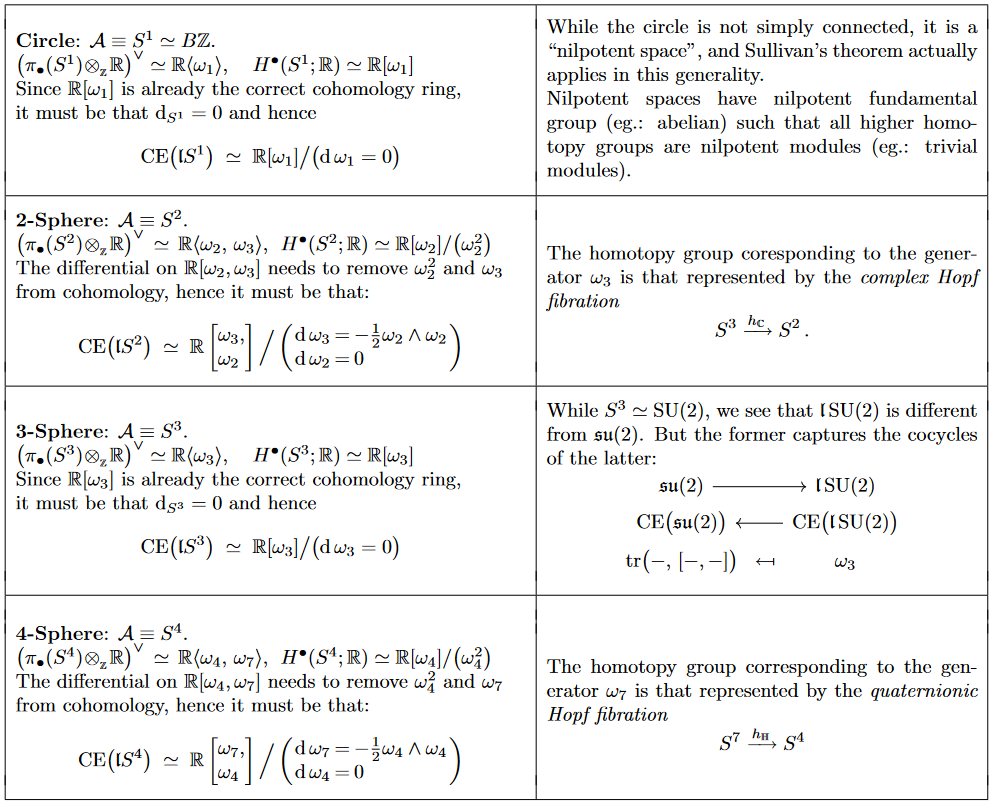
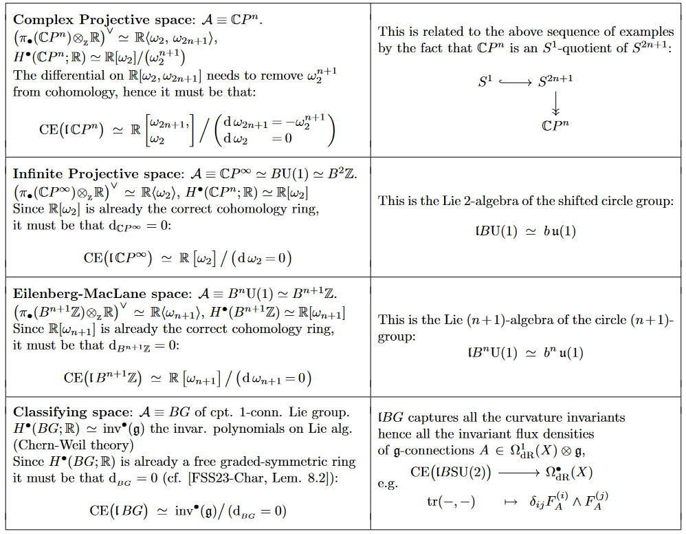
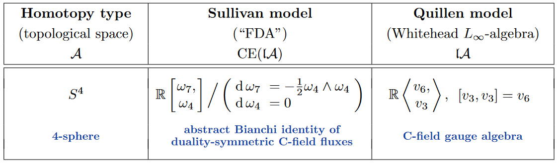
Many of the Whitehead $L_\infty$-algebras of familar spaces do not have established names as $L_\infty$-algebras. An interesting exception is the Whitehead $L_\infty$-algebra of the 4-sphere, which happens to coincide with what in D=11 supergravity-theory is known (quite independently) as the gauge algebra of the C-field [Cremmer, Julia, Lu & Pope 1998, (2.6); Sati 2010, §4; Sati & Voronov 2022, (13)] (see more references there):

Remark

(prefactors in Sullivan algebras)
As stated so far, the ubiquituous prefactor $-\tfrac{1}{2}$ is pure convention, due to the freedom of rescaling generators by rational (or even real) numbers while retaining dga-isomorphy. However, this factor is fixed by requiring certain integrality properties of the generators, see FSS21-HopfWZ, Prop. 4.6.

This becomes relevant when regarding the lift back from $\mathfrak{l}S^4$ to $\mathcal{A} \equiv S^4$ as a flux quantization law, because then it implies that the C-field flux densities $G_4$ and $G_7$ in the image of the normalized generators $\omega_4$ and $\omega_7$ satisfy expected integrality conditions [FSS21-HopfWZ, Thm. 4.8]. We discuss this further below.

Rational homotopy theory: Discrading torsion in nonabelian cohomology. From the perspective (above) that any topological space $\mathcal{A}$ serves as the classifying space of a generalized nonabelian cohomology theory, the idea of rational homotopy theory (survey in Hess 2006; FSS23-Char, §4) becomes that of extracting the non-torsion content of such a cohomology theory, which we will see is, over smooth manifolds, that shadow of it that is reflected in the non-abelian de Rham cohomology (Def. ) of $\mathfrak{l}\mathcal{A}$-valued differential forms.

Hence to have a classifying space for the non-torsion part of $\mathcal{A}$-cohomology means to ask for:

(23)

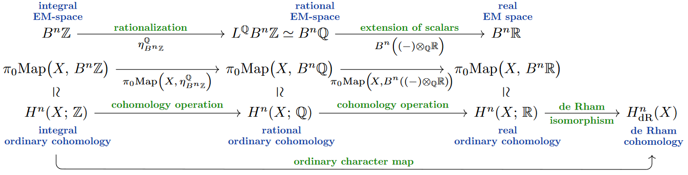
For example, the rationalization of an integral Eilenberg-MacLane space $B^n \mathbb{Z} \,\equiv\, K(\mathbb{Z},n)$ classifies ordinary rational cohomology, mapping to ordinary de Rham cohomology:

We may regard this as the archetype of a character map and ask for its generalization to any $\mathcal{A}$-cohomology theory. The pivotal observation of FSS23-Char is that for this purpose one may invoke the fundamental theorem of dg-algebraic rational homotopy theory:

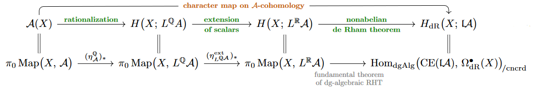
The Fundamental Theorem of dg-Algebraic Rational Homotopy Theory (review in FSS23-Char, Prop. 5.6) says that the homotopy theory of rational spaces (simply-connected with fin-dim rational cohomology) is all encoded by their Whitehead $L_\infty$-algebras (22) over the rational numbers.

In particular, for $X$ a CW-complex, the homotopy classes of maps into the rationalization $L^{\mathbb{Q}}\mathcal{A}$ (23) of a space $\mathcal{A}$ is identified with dg-homotopy classes of homomorphisms from the rational Sullivan model of $\mathcal{A}$ to the “piecewise polynomial de Rham complex” of the topological space $X$:

(24)

Observing that the right-hand side looks close to the definition of $\mathfrak{l}\mathcal{A}$-valued de Rham cohomology (Def. ), in order to actually connect to such smooth differential forms one needs to extend the ground field scalars from the rational numbers to the real numbers:

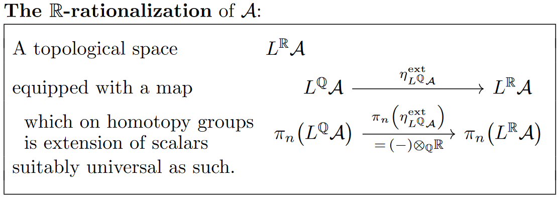
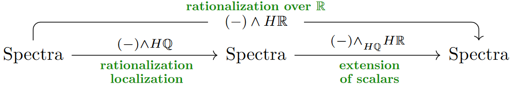
$\;\;$Rational homotopy theory over the Reals. [Bousfield & Gugenheim 1976; reviewed in FSS23-Char, Def. 5.7, Rem. 5.2, Prop. 5.8] The construction (23) also works over $\mathbb{R}$ (but is then not a “localization”) to give the $\mathbb{R}$-rationalization.

With this “derived extension of scalars” [FSS23-Char, Lem 5.3] and for $X$ a smooth manifold, the fundamental theorem (24) does relate to smooth differential forms [FSS23-Char, Lem. 6.4] via a non-abelian de Rham theorem [FSS23-Char, Thm. 6.5]:

(25)

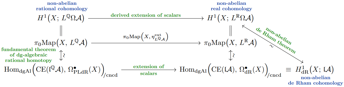
In abelian (ie. Whitehead-generalized) cohomology theories both the rationalization step and the subsequent extension of scalars to $\mathbb{R}$ can be more easily described as forming the smash product of the coefficient spectrum with the rational Eilenberg-MacLane spectrum $H\mathbb{R}$ [FSS23-Char, Ex. 5.7]. This is how the Chern-Dold character map over $\mathbb{R}$ is tacitly used in all the literature on abelian (Whitehead-generalized) differential cohomology theory (e.g. Bunke & Nikolaus 2014, Def. 4.2):

(26)

The point of the non-abelian de Rham theorem (25) is to generalize the realifification (26) of Whitehead-generalized cohomology to generalized non-abelian cohomology, such as to Cohomotopy; and the key result that makes this work is the fundamental theorem of dg-algebraic homotopy theory (24). This, ultimately, is the “reason” why $L_\infty$-valued differential forms relate fluxes to their flux-quantization laws.

The general non-abelian character map is now immediate [FSS23-Char, Def. IV.2]: It is the cohomology operation induced by $\mathbb{R}$-rationalization of classifying spaces, seen under the non-abelian de Rham theorem (25):

(27)

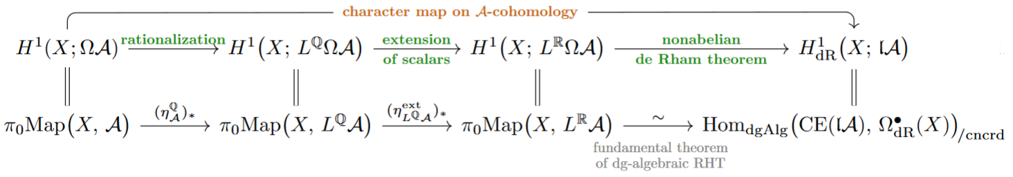
All the classical abelian character maps (21) are special cases of this generalized nonabelian character [FSS23-Char, §7], but now examples in generalized nonabelian cohomology are also included; for instance there is a character map on Cohomotopy-theory [FSS23-Char, Ex. 6.11]

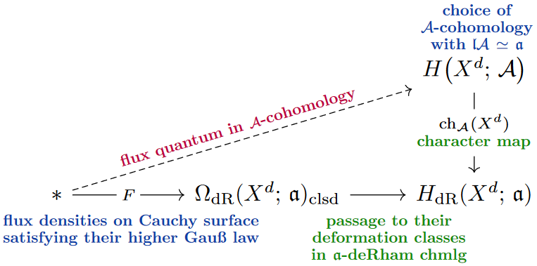
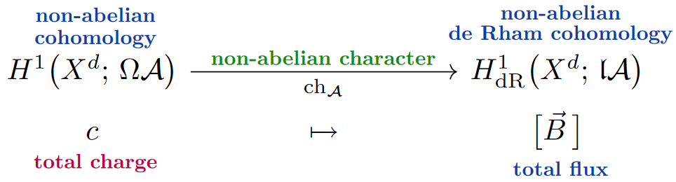
Flux quantization in generalized nonabelian cohomology. With the generalized nonabelian character map (27) in hand, we may finally state the general concept of flux quantization (to be further refined below):

Recalling (20) that the $\mathfrak{a}$-valued nonabelian de Rham cohomology of a Cauchy surface encodes the total flux of the higher gauge fields characterized by the $L_\infty$-algebra $\mathfrak{a}$, it follows that for every choice of classifying space $\mathcal{A}$ with $\mathfrak{l}\mathcal{A} \,\simeq\, \mathfrak{a}$ the nonabelian character map (27) may be understood as assigning to discrete charges embodied by $\mathcal{A}$-cohomology-classes the corresponding total flux (thereby losing torsion-information encoded in the charges but not in the fluxes):

(28)

Since the total charges in $H^1\big(X^d; \Omega \mathcal{A})\big)$ on the left form a discrete set, we may think of implementing global flux quantization in $\mathcal{A}$-cohomology as lifting of total fluxes through the character map:

Notice that such a lift is not just a (quantization/discretization-)condition on the total fluxes, but also extra structure, namely a choice of torsion-component of the total charge reflected in total fluxes, as see in $\mathcal{A}$-cohomology:

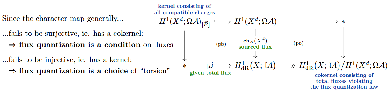
However, in a higher gauge theory it is unnatural to have extra structure given by an equality of gauge equivalence classes, instead one should consider an explicit gauge transformation between actual fields. Doing so leads to emergence of the gauge potentials and of the higher phase space stack of the theory, in the next subsection.

Example

(flux quantization laws for ordinary electromagnetism)

By Ex. the characteristic $L_\infty$-algebra of vacuum electromagnetism is two copies of the line Lie 2-algebra $b \mathfrak{u}(1)$. This is the Whitehead $L_\infty$-algebra of the classifying space $B \mathrm{U}(1)$$\,\simeq\, B^2 \mathbb{Z}$ and hence of its rationalization $B^2 \mathbb{Q}$.

Therefore – among many further variants – there are the following choices of flux quantization laws for electromagnetism:

EM flux quantization law	comment
$\underset{mag}{\underbrace{B^2 \mathbb{Q}}} \,\times\, \underset{el}{\underbrace{B^2 \mathbb{Q}}}$	this choice imposes no flux quantization (it does rule out irrational total fluxes) and as such was the tacit choice since Maxwell 1865 until Dirac 1931
$\underset{mag}{\underbrace{B^2 \mathbb{Z}}} \,\times\, \underset{el}{\underbrace{B^2 \mathbb{Q}}}$	this choice imposes integrality of magentic charge but no further condition on electric flux – common choice since Dirac 1931, for instance in Alvarez 1985b, p. 299; Brylinski 1993, §7.1; Freed 2000, Ex. 2.1.2
$\underset{mag}{\underbrace{B^2 \mathbb{Z}}} \,\times\, \underset{el}{\underbrace{B^2 \mathbb{Z}}}$	this choice imposes integrality of both magentic and electric charges – considered in Freed, Moore & Segal 2007a, 2007b; Becker, Benini, Schenkel & Szabo 2015, Rem. 2.3; Lazaroiu & Shahbazi 2022; Lazaroiu & Shahbazi 2023, §2
$\underset{mag}{\underbrace{B^2 \mathbb{Z}}} \,\rtimes\, \underset{el}{\underbrace{B\big( K \ltimes B\mathbb{Z} \big) }}$	for a finite group $K \to Aut(\mathbb{Z})$ – this choice induces non-commutativity between EL/EL- and EL/M-fluxes, an example of a “non-evident” flux quantization condition considered in SS23-FQ

Phase spaces as Differential nonabelian cohomology

With higher Maxwell-type equations of flux given (above) and with a compatible flux/charge quantization law $\mathcal{A}$ chosen (above), we explain here how the full on-shell field content of the higher gauge theory (including the gauge potentials) and hence its phase space (13) appears as the corresponding “moduli space” of nonabelian differential cohomology $\widehat{A}$ of any Cauchy surface.

In fact, such a phase space is not just a smooth manifold, but is a smooth $\infty$-groupoid (aka smooth $\infty$-stack, hence a higher moduli stack) whose higher morphisms represent the higher gauge transformations between the field configurations; and so we briefly review some required concepts from higher topos theory (for full details we refer the reader to FSS23-Char, §1 & §9, quick exposition of the basic ideas is in Schreiber 2024).

However, the “topological observables” on the higher gauge theory (those that detect topological charge structure but not the local differential geometry of field configurations) depend only on the “shape” of the phase space stack, which by the properties of “cohesive higher topos theory” turns out to coincide simply with the actual mapping space from the Cauchy surface into the classifying space $\mathcal{A}$.

Therefore the reader who is not to be bothered with higher topos theory and is content with the “topological” implications of flux quantization may safely (dis-)regard this subsection as a black box which guarantees that once a classifying spaces $\mathcal{A}$ is chosen for flux quantization, it controls not only the set $H^1\big(X^d;\, \mathcal{A}\big) \,\equiv\, \pi_0 Map(X^d, \mathcal{A})$ of total charges of the theory, but also the full moduli space $Map(X^d, \mathcal{A})$ of local charges.

Smooth sets of moduli of flux densities.

The idea of moduli stacks is the evident refinement of that of classifying spaces: Given a certain kind of structure (in physics typically: a certain kind of fields):

1. a classifying space is such that homotopy classes of (continuous) maps to it from any $X$ correspond to equivalence classes of such structures on $X$,

2. a moduli stack is such that the individual (smooth) maps to it from any $X$ correspond to the individual such structures on $X$,

   with (higher) homotopies of these maps corresponding to the (higher) gauge transformations between these structures.

In order to understand that and how such moduli stacks may exist at all, it is useful to take a perspective where every kind of space under consideration (such as spacetime itself) is defined (not as an underlying set of points with extra structure but) by the maps it receives from given probes.

$\;$Smooth sets. We refer the reader to the section geometry of physics – smooth sets or else to [Giotopoulos & Sati 2023] for more exposition and discssion of the following idea:

For the present purpose of higher differential geometry, the relevant probe spaces are “abstract coordinate charts”, namely Cartesian spaces $\mathbb{R}^n$, and the idea is that any space $X$ which qualifies as a “smooth set” should be defined (not necessarily by an underlying set of points equipped with smooth structure but) by a system of sets of ways

(29)$$\mathbb{R}^n \;\mapsto\; Plots\big( \mathbb{R}^n ,\, X \big)$$

of plotting out probe spaces $\mathbb{R}^n$ inside the would-be space $X$. Basic consistency requirements demand that this assignment should make a contravariant functor to Sets (a “presheaf”)

$$Plots\big( -; X \big) \;\colon\; CartSp^{op} \longrightarrow Set$$

from/on the category CartSp of Cartesian spaces $\mathbb{R}^n$ ($n \in \mathbb{R}$) with smooth functions between them. Similar considerations show that a smooth map $f \,\colon\, X \to Y$ between smooth sets defined this way (only) by their systems of plots should be just a compatible system of transformations of plots-of-$X$ to plots-of-$Y$, hence should be a natural transformation between such functors.

The further consistency requirement of locality of probes demands that such a smooth map $f \,\colon\, X \to Y$ should “count as” an invertible isomorphism (diffeomorphism of smooth sets) already if it is a local isomorphism in that its transformation $f_\ast$ of plots is a bijection (not necessarily on all plots but) between germs of plots (around $0 \in \mathbb{R}^n$, say, hence a bijection on “stalks” at $0$).

This way one find that the category of smooth sets should be the “localization” $L^{iso}$ of the category of presheaves on CartSp at the stalk-wise bijections hence at the “local isomorphisms” ($liso$), also known as the category of sheaves or the sheaf topos over the site CartSp:

(30)$$SmoothSet \;\coloneqq\; Sh(CartSp) \;\simeq\; L^{liso} PSh(CartSp) \,.$$

For example, if $X$ is an ordinary smooth manifold then it is regarded as a smooth set by taking its plots to be the actual smooth functions into it:

$$\array{ SmthMfd &\hookrightarrow& SmoothSet \\ X &\mapsto& \underset{ Plot(-;X) }{\underbrace{C^\infty(-;X)}} }$$

In particular, the probe Cartesian spaces $\mathbb{R}^n$ are incarnated themselves as smooth sets in this way. This allows to compare the prescribed plots $Plot(\mathbb{R}^n,X)$ of any smooth set with the actual smooth maps $Hom\big(\mathbb{R}^n, X \big)$ into it (forming the hom-sets of SmoothSet), and remarkably they coincide (this is the Yoneda lemma over CartSp), thus rendering consistent the above “bootstrap definition” of smooth sets:

$$\left. \begin{array}{l} X \in SmoothSet \\ \mathbb{R}^n \in CartSp \end{array} \; \right\} \;\;\;\;\;\;\; \vdash \;\;\;\;\;\;\; \array{ Hom\big(\mathbb{R}^n,\, X\big) &\overset{\sim}{\longrightarrow}& Plot\big(\mathbb{R}^n,\, X\big) \\ f &\mapsto& f_\ast id_{\mathbb{R}^n} \,. }$$

But the category SmoothSet contains now much more than just ordinary smooth manifolds, in particular it contains (0-truncated) moduli stacks of differential forms:

For $p \in \mathbb{N}$, the smooth differential n-forms clearly form a sheaf over CartSp and hence may be regarded as the plots of a smooth set $\mathbf{\Omega}^p_{dR} \,\in\, SmoothSet$:

$$Plot\big( \mathbb{R}^n ,\, \mathbf{\Omega}^p_{dR} \big) \;\; \coloneqq \;\; \Omega^p_{dR}(\mathbb{R}^n) \,.$$

One checks that this is a moduli stack for differential forms on smooth manifolds, in that for $X \in SmthMfd \hookrightarrow SmthSet$ we have a natural bijection

(31)$$X \in SmthMfd \hookrightarrow SmthSet \;\;\;\;\;\;\; \vdash \;\;\;\;\;\;\; Hom\big( X ,\, \mathbf{\Omega}^p_{dR} \big) \;\simeq\; \Omega^p_{dR}(X)$$

of the smooth maps from $X$ into $\mathbf{\Omega}^p_{dR}$ with the actual smooth differential forms.

Here it is useful to think of $\mathbf{\Omega}^p_{dR}$ as a space which carries a universal differential $p$-form $\omega_p^{univ} \,\in\, \Omega^p_{dR}\big(\mathbf{\Omega}^p_{dR}\big)$ (as befits a moduli stack of differential forms) such that every differential form on any $X$ is the pullback of $\omega_p^{univ}$ along a unique smooth map $X \to \mathbf{\Omega}^p_{dR}$.

In fact, it makes sense to define differential forms on any smooth set by

$$X \,\in\, SmthSet \;\;\;\;\;\;\; \vdash \;\;\;\;\;\; \Omega^p_{dR}(X) \;\coloneqq\; Hom\big( X ,\, \mathbf{\Omega}^p_{dR} \big)$$

and then that universal differential form on $\mathbf{\Omega}^p_{dR}$ actually exists:

$$\omega_p^{univ} \;\coloneqq\; id \,\in\, Hom\big( \mathbf{\Omega}^p_{dR} ,\, \mathbf{\Omega}^p_{dR} \big) \;\equiv\; \Omega^p_{dR}\big( \mathbf{\Omega}^p_{dR} \big) \,.$$

It is in this way that the category SmoothSet makes (0-truncated) moduli stacks exist in just the way they ought to (and higher moduli stacks exist similarly in the higher generalization of smooth sets to smooth infinity-groupoids that we turn to below).

For the case at hand, it is now straightforward to further specialize this example: The (0-truncated) moduli stack of flat $\mathfrak{a}$-valued differential forms for a given $L_\infty$-algebra $\mathfrak{a}$ is the smooth set whose plots are just those differential forms on Cartesian spaces

(32)$$\Omega^1_{dR}(\text{-};\mathfrak{a})_{clsd} \;\in\; SmthSet$$

and in generalization of (31), this is again the moduli stack of such differential forms in that:

(33)$$X \in SmthMfd \hookrightarrow SmthSet \;\;\;\;\;\;\; \vdash \;\;\;\;\;\;\; Hom\big( X ,\, \Omega^1_{dR}(\text{-};\mathfrak{a})_{clsd} \big) \;\simeq\; \Omega^p_{dR}(X) \,.$$

Simplicial sets of moduli of charges.

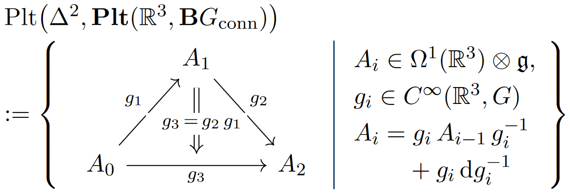
But independently of the differential geometry, the collection of fields in a higher gauge theory is not really a set with unambiguously distinct elements: A pair $\Phi$, $\Phi'$ of gauge fields may be distinct and yet identified by gauge transformations $\Phi \underoverset{\sim}{g}{\longrightarrow} \Phi'$. Moreover, for higher gauge fields there is not really a set of such gauge transformations either, as any pair of them, in turn, may be distinct and yet identified by a gauge-of-gauge transformation $\mu$, etc.

There are different equivalent ways to record systems of such higher gauge transformations. A globular or cubical arrangement suggests itself but turns out to come with technical subtleties, while the “simplicial” arrangement indicated above turns out to be remarkably useful and has an extremely well-developed theory: Here the gauge-of-gauge transformations are always taken to fill a triangle of ordinary gauge transformations, the next higher gauge transformations are taken to fill a tetrahedron of these, and generally an $n$-gauge transformation is taken to form the $n$-dimensional generalization of tetrahedra, called $n$-simplices. Notice that this subsumes the intuitively expected “globular” situations by taking some faces of the simplices to be labeled by identity-transformations, as indicated on the right.

Hence (still disregarding its differential geometry) the underlying set of fields of a higher gauge theory is, beyond the “0-simplices” of the nominal fields themselves, actually a system of sets of higher simplices of higher gauge transformations in any dimension, such that with any $n$-simplex also all its face $(n-1)$-simplices and all the correspoinding “thin” (“degenerate”) $(n+1)$-simplices are part of this simplicial set:

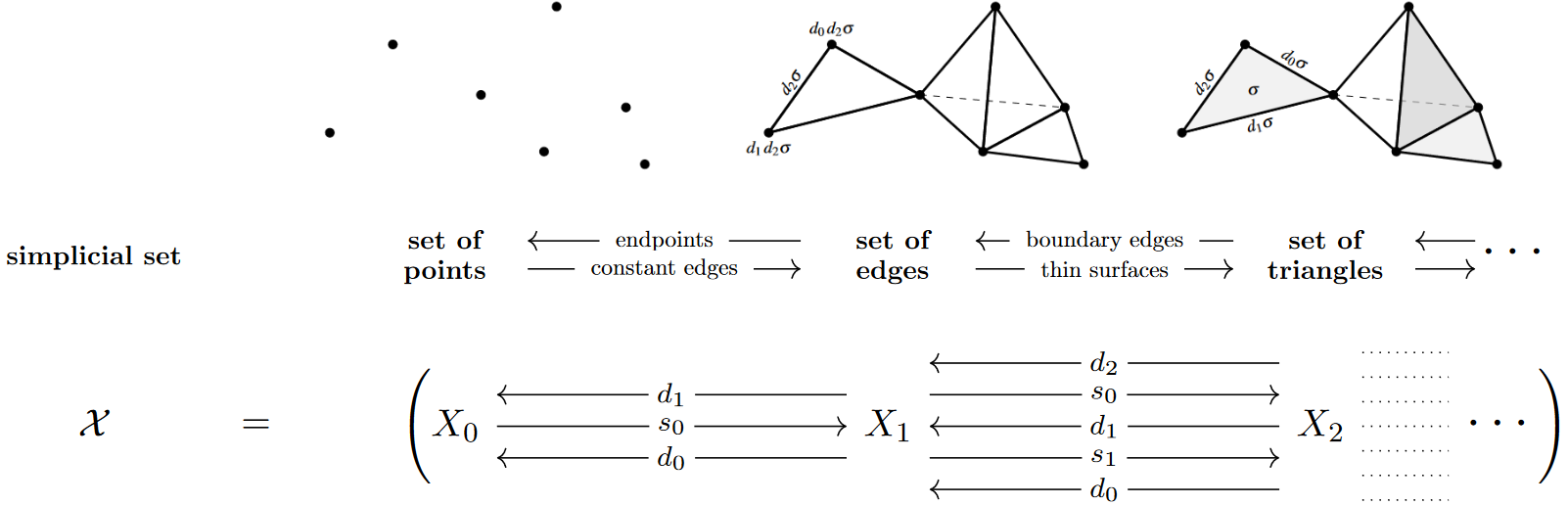
Hence — in the spirit (29) of generalized spaces defined by how to plot out probe-spaces inside them —, such simplicial sets are those generalized spaces which are probe-able by the abstract cellular simplices $\Delta^n$ forming the simplex category $\Delta$, and hence the category SimpSet of simplicial sets is that of presheaves on $\Delta$:

$$SimpSet \;\coloneqq\; PSh(\Delta) \,.$$

For example, given a Lie group $G$ with Lie algebra $\mathfrak{g}$ then the groupoid of $G$-Yang-Mills gauge potentials on $\mathbb{R}^3$ – to be denoted $\mathbf{Plt}(\mathbb{R}^3,\mathbf{B}G_{conn})$ for reasons discussed below – is the simplicial set whose:

0-Simplices are the YM gauge potentials, hence the $\mathfrak{g}$-valued 1-forms $A \in \Omega^1_{dR}(\mathbb{R}^3; \mathfrak{g})$;

1-Simplices are the smooth $G$-valued functions $g \,\colon\, \mathbb{R}^3 \to G$ serving as gauge transformations between such gauge potentials;

2-Simplices are uniquely filled whenever the gauge transformations around their boundary compose;

$n\geq 3$-Simplices are uniquely filled whenever their face $(n-1)$-simplices exist.

That this example is indeed a groupoid in that the gauge transformation 1-simplices have inverses and composites (whenever composable) is witnessed by the fact that whenever one finds in this simplicial set a pair of 1-simplices that share a 0-simplex (jargon: a “2-horn” $\Lambda^2_i$) then there exists a 2-simplex completing the diagram.

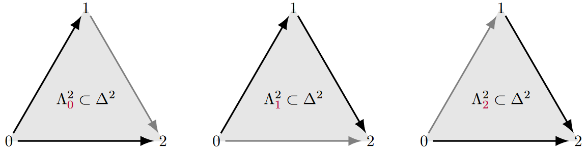
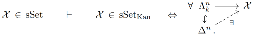
Similarly one defines the higher horns $\Lambda^n_i \subset \Delta^n$ to be the sub-simplicial sets of a simplex missing the interior and the $ith$ face, and then says that a simplicial set is an $\infty$-groupoid (historical terminology: Kan complex) if all images of $\Lambda^n_i$ inside it may be completed to an images of $\Delta^n$.:

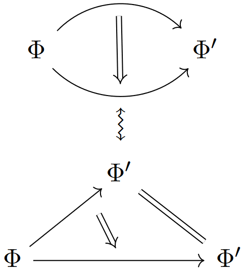
As an abstract class of examples: For $\mathcal{X},\, \mathcal{Y} \,\in\, SimpSet_{Kan}$, there is the $\infty$-groupoid of maps between them $Map(\mathcal{X},\mathcal{Y})\,\in\, SimpSet_{Kan}$, whose $\Delta^n$-shaped plots are the $\Delta^n$-parameterized systems of simplicial maps

(34)$$Plt\big( \Delta^n ,\, Map(\mathcal{X},\mathcal{Y}) \big) \;\coloneqq\; Hom\big( \Delta^n \times \mathcal{X} ,\, \mathcal{Y} \big) \,,$$

hence whose 0-simplices are the plain maps $\mathcal{X} \to \mathcal{Y}$ and whose 1-simplices are homotopies between such maps.

(35)

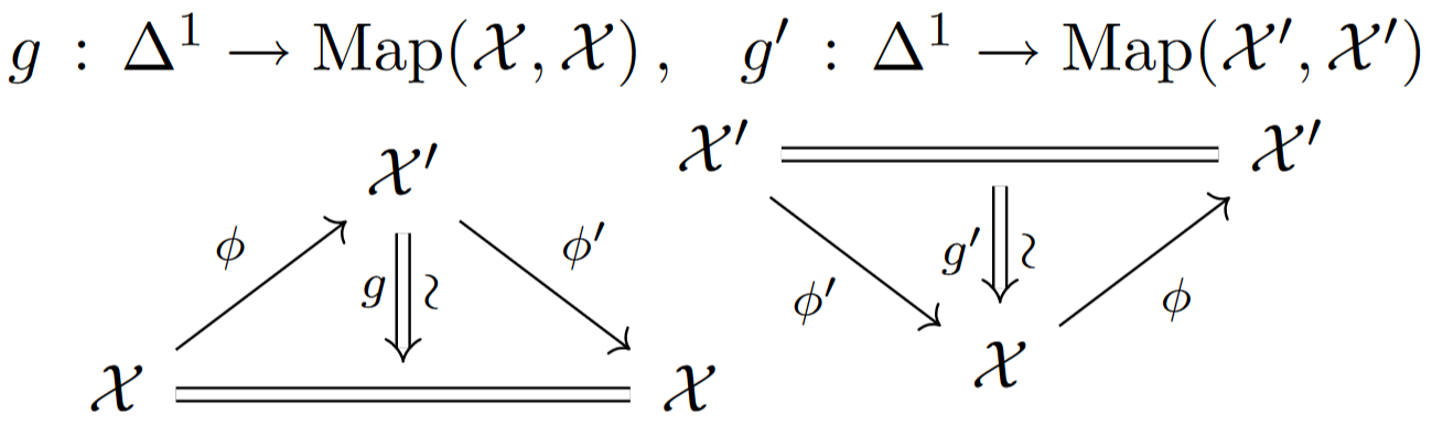
Hence a homotopy equivalence between $\infty$-groupoids consiste of maps back and forth which are inverses up to homotopy (in that there exist homotopies $g$, $g'$ as shown).

(Beware that if one works with all simplicial sets instead of just the Kan-simplicial sets among them, as often done in the literature, then the relevant notion of equivalence is instead “weak homotopy equivalence”.)

As a more concrete class of examples: A topological space $X$ gives rise to an $\infty$-groupoid $\esh X \,\in\, SimpSet_{Kan}$: its path infinity-groupoid whose $n$-morphisms are the continuous images of the geometric $n$-simplices $\Delta^n_{geo}$ in $X$:

(36)$$\begin{array}{l} Plot\big( \Delta^n ,\, \esh X \big) \\ \;\coloneqq\; Hom_{Top}\Big( \; \underset{ \Delta^n_{geo} \phantom{ \vert^{\vert^{\vert}} } }{ \underbrace{ \big\{ \vec x \in (\mathbb{R}_{\geq 0})^{\times^{n+1}} \,\big\vert\, \textstyle{\sum}_i x^i = 1 \big\} } } \, ,\, X \Big) \,. \end{array}$$

(37)

This path $\infty$-groupoid-construction forgets the topology on $X$ (the “cohesion” of its points as embodied by its system of open subsets) but retains the shape of $X$, namely its homotopy type: The equivalence class of $\esh X$ under homotopy equivalences (35). A classical fact of homotopy theory asserts (in particular) that every homotopy type in $SimpSet_{Kan}$ is equivalently the shape/path $\infty$-groupoid of some topological space, which traditionally leads to some conflation of these different notion of “space”.

Here we shall denote actual homotopy types $\mathcal{X} \,\in\, SimpSet_{Kan}$ by calligraphic symbols. In particular, it is homotopy types $\mathcal{A}$ which determine flux quantization laws above:

The plain (as opposed to differential) nonabelian cohomology (above) of a topological space $X$ is an invariant of its shape/homotopy type $\esh X$ (36) formed by the simplicial mapping complex (34):

(38)$$\left. \begin{array}{l} \mathcal{A} \,\in\, SimpSet_{Kan} \\ X \,\in\, Top \end{array} \; \right\} \;\;\;\;\;\;\; \vdash \;\;\;\;\;\;\; H^1(X;\, \mathcal{A}) \;\; \simeq \;\; \pi_0 Map\big( \esh X ,\, \mathcal{A} \big) \,,$$

where on the right $\pi_0(-)$ refers to the connected components of an $\infty$-groupoid $\mathcal{X} \,\in\, SimpSet_{Kan}$ being the quotient set of the 0-simplices by the equivalence relation embodied by the 1-simplices: $\pi_0 \mathcal{X} \;\coloneqq\; \mathcal{X}_0\big/\mathcal{X}_1$.

While above we saw that any cohomology class $[\chi] \,\in\, H^1\big(X;\, \mathcal{A}\big)$ may be understood as the total charge sourcing $\mathfrak{l}\mathcal{A}$-valued flux, next we may use differential homotopy theory in order to regard actual representative maps $\esh X \to \mathcal{A}$ as witnessing the local charge, in a sense, which may be regarded as the source not just of a total flux in $H^1\big(X;\, \mathfrak{l}\mathcal{A}\big)$ but an actual locally defined flux density $\vec B$.

Smooth simplicial sets of deformations of flux densities. With the above discussion one has moduli for

1. flux densities with their differential geometric nature, in SmoothSet,

2. local charges with their higher gauge theoretic nature, in SimpSet.

In order to discuss moduli for the full flux-quantized fields, one need to combine these two aspects into a category of smooth simplicial sets (smooth Kan-simplicial sets, to be precise).

It is clear that these should be presheaves on CartSp with values in Kan-simplicial sets, subject to their combined notion of equivalence: local equivalences as for smooth sets (30) and homomotopy equivalences as for $\infty$-groupoids (35):

For $\mathcal{X}, \mathcal{Y} \,\in\, PSh\big(CartSp,\, SimpSet_{Kan}\big)$ a morphism $f \,\colon\, \mathcal{X} \to \mathcal{Y}$ is a local homotopy equivalence (lheq) if it is a morphism that restricts to a homotopy equivalence (35) on all germs of plots, hence on all simplicial stalks.

To regard these local homotopy equivalences as the actual equivalences of smooth simplicial sets means to pass to the simplicial localization of the category of smooth simplicial sets at the local homotopy equivalences, to be denoted:

(39)$$SmthGrpd_\infty \;\coloneqq\; \mathbf{L}^{\!lheq} \, SmoothSimpSet_{Kan} \;\coloneqq\; \mathbf{L}^{\!lheq} \, PSh\big( CartSp ,\, SimpSet_{Kan} \big)$$

and referred to as the $\infty$-topos of smooth $\infty$-groupoids.

It is clear that, both, smooth sets as well as plain $\infty$-groupoids are jointly contained in this larger category, the former as the objects which are constant on $\Delta$ (the 0-truncated objects) and the latter as the objects which are constant on $CartSp$ (the geometrically discrete objects). This allows to put both flux densities as well as the (homotopy types of) charge classifying spaces $\mathcal{A}$ on the same footing and hence relate them to each other fur the purpose of flux quantization, as previewed in the following diagrsm:

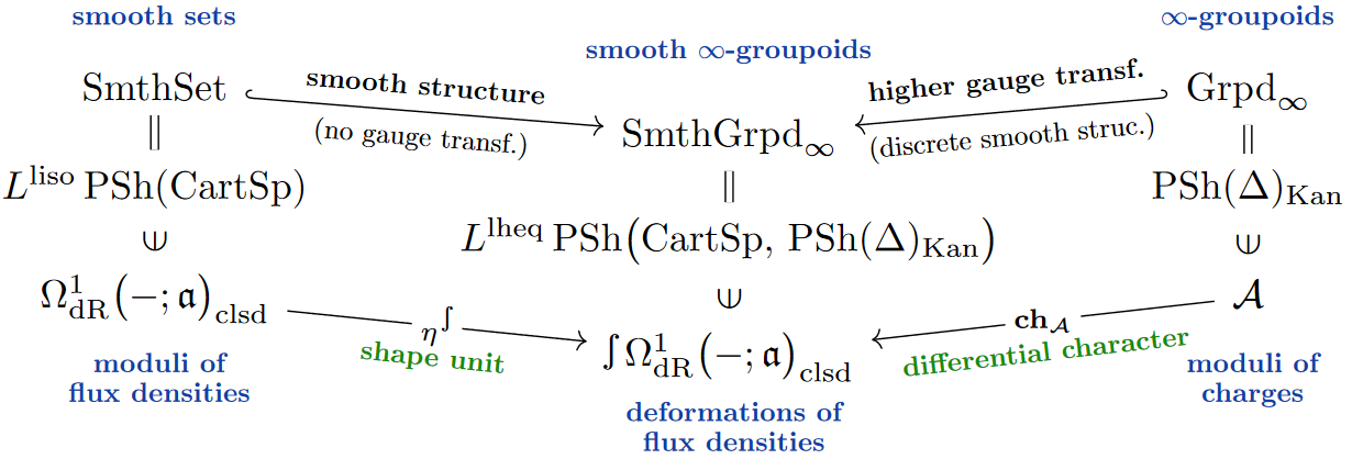
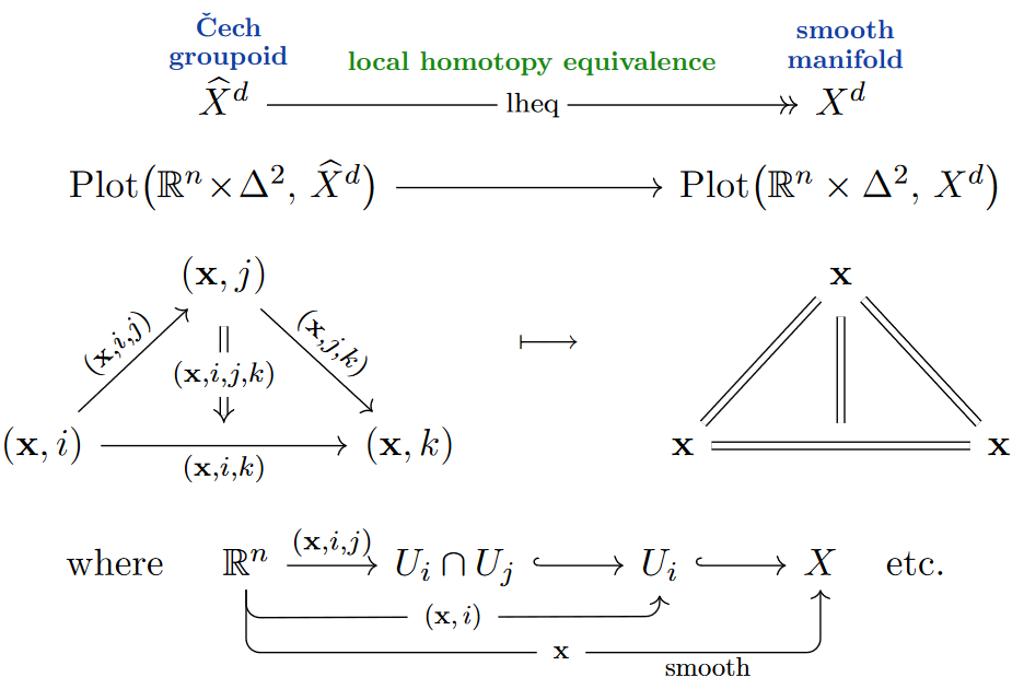
As an example of a local homotopy equivalence of smooth simplicial sets, consider a smooth manifold $X^d$ and $\big\{\mathbb{R}^d \simeq U_j \xhookrightarrow{ \iota_j } X \big\}_{j \in J}$ a good open cover. Then the Čech groupoid $\widehat X{}^d \,\in\, SmoothSimpSet_{Kan}$ has as $\Delta^n$-shaped plots the smooth maps into the $(n+1)$-fold intersections of the open patches:

(40)$$\begin{array}{l} Plot\Big( \mathbb{R}^n \times \Delta^n ,\, \widehat{X}{}^d \Big) \\ \; \coloneqq \; C^\infty\big( \mathbb{R}^n ,\, \underset{ j_\bullet \in J^{n+1} }{ \textstyle{\coprod} } \, U_{j_0} \cap \cdots \cap U_{j_n} \big) \,. \end{array}$$

Since the patches are subsets of $X^d$, this has an evident map to $X^d$ which is readily seen to be a local homotopy equivalence.

Since this map $\widehat X{}^d \to X^d$ becomes invertible in (39), maps in $SmoothGrpd_\infty$ out of $X^d$ are the same as maps out of $\widehat X{}^d$. But some further theory shows that $\widehat X{}^d$ is a good (namely: cofibrant) representative of the local homotopy equivalence class of $X^d$, in that maps out of it may be considered already before localization, in $SmoothSimpSet_{Kan}$.

This is important, because for any $\infty$-groupoid $\mathcal{A} \,\in\, SimpSet_{Kan} \xhookrightarrow{const} SmoothSimpSet_{Kan}$ regarded as a geometrically discrete smooth $\infty$-groupoid, the nonabelian cohomology $H^1\big(X;\, \Omega\mathcal{A}\big)$ (41) may equivalently be computed as the special case of “differential” cohomology of smooth $\infty$-groupoids with coefficients that happen to be non-differential (geometrically discrete)

(41)$$\left. \begin{array}{l} \mathcal{A} \,\in\, SimpSet_{Kan} \\ X^d \,\in\, SmthMfd \end{array} \; \right\} \;\;\;\;\;\;\; \vdash \;\;\;\;\;\;\; H^1(X;\, \mathcal{A}) \;\; \simeq \;\; \pi_0 Map\big( \, \widehat X{}^d ,\, \mathcal{A} \, \big) \,,$$

In components this is the Čech cohomology-presentation of generalized nonabelian cohomology.

On the other hand, if the target object is a smooth set such as $\Omega^1_{dR}(-;\mathfrak{a})_{clst}$ (32) then smooth simplicial maps out of the Čech groupoid into it collapse to maps out of just $X$ itself.

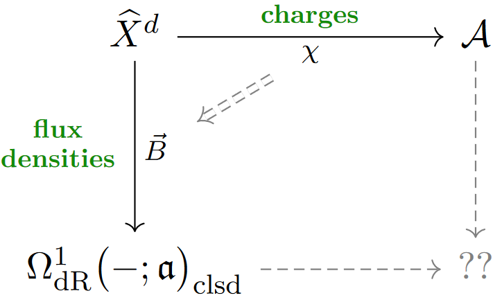
In summary so far, this means that flux densities as well as their local charges are now both “modulated” by maps of smooth $\infty$-groupoids:

In order to impose flux quantization – hence the condition that these $\mathfrak{a}$-flux densities are sourced by such $\mathcal{A}$-charges – it remains to construct moduli stack in which both these components may be universally related:

Higher deformations of flux densities. Recall (20) that a coboundary in $\mathfrak{a}$-valued de Rham cohomology is a “concordance” of flux densities, to be thought of as a path of smooth variations of the flux densities subject to their Bianchi identities:

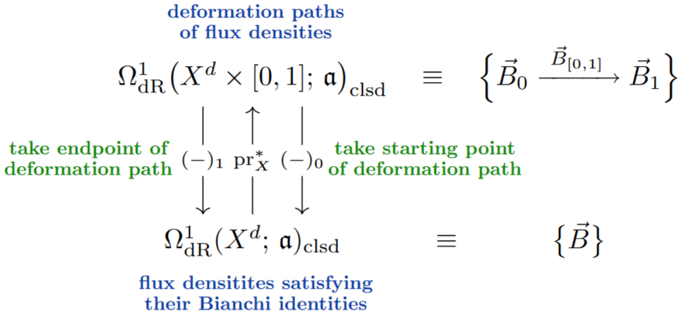
Here $[0,1] \simeq \Delta^1_{geo}$, and in higher gauge theories there are also non-trivial deformations-of-deformations varying over the higher dimensional $n$-simplices $\Delta^n_{geo}$:

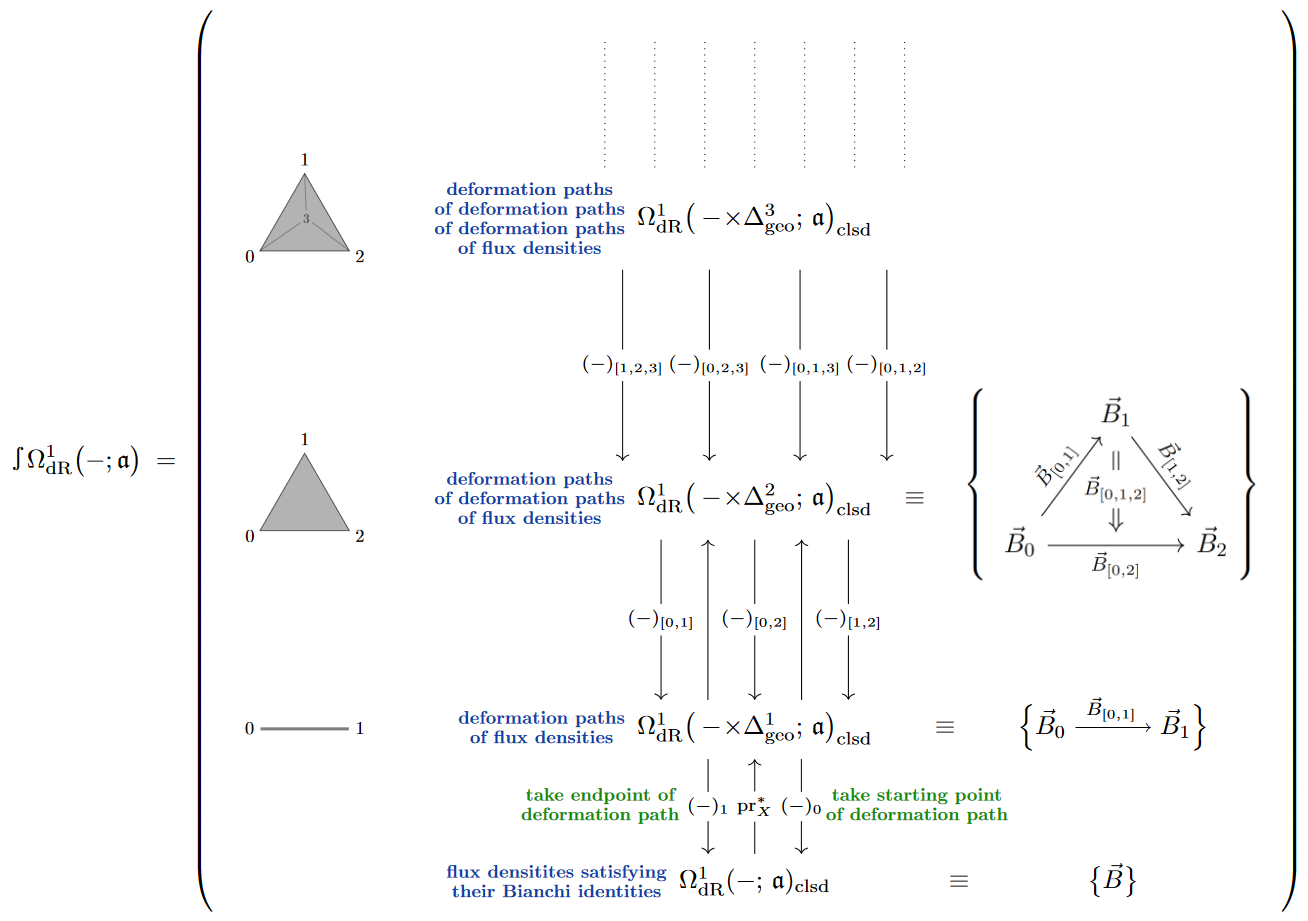
Since in each degree this is a set of plots of a smooth set of on-shell flux densities (32), we have in total a smooth simplicial set [FSS23-Char, Def. 9.1] that is Kan [FSS23-Char, Prop. 5.10] and which we may think of as the shape or smooth path $\infty$-groupoid of the moduli of flux densities:

$$\esh \, \Omega^1_{\mathrm{dR}}\big( -; \mathfrak{a} \big)_{clsd} \;\in\; SmoothSimpSet_{Kan} \,.$$

It is in this object that flux densities become comparable to their charges:

(1.) There is the evident inclusion of the smooth set of flux densities [FSS23-Char (9.3)]

$$\Omega^1_{\mathrm{dR}}\big( -; \mathfrak{a} \big)_{clsd} \xrightarrow{ \;\; \eta^{\esh} \;\; } \, \Omega^1_{\mathrm{dR}}\big( -; \mathfrak{a} \big)_{clsd} \,.$$

(2.) Given an identification $\mathfrak{a} \,\simeq\, \mathfrak{l}\mathcal{A}$ with a Whitehead $L_\infty$-algebra (Prop. ), then the fundamental theorem of dg-algebraic rational homotopy theory (24) furthermore says [FSS23-Char, Lem. 9.1] that we have a (homotopy-)equivalence to the $\mathbb{R}$-rationalization $L^{\mathbb{R}} \mathcal{A}$ of $\mathcal{A}$ (above) so that rationalization gives a differential character map [FSS23-Char, Def. 9.2]

(42)

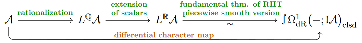
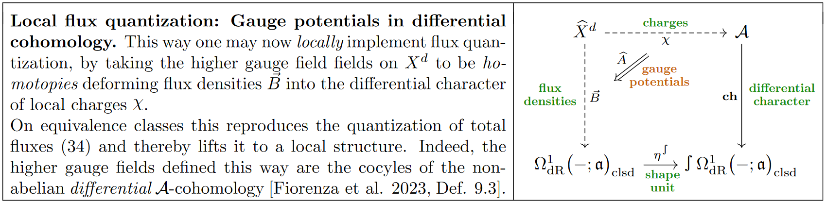
These homotopies turn out to reflect the expected gauge potentials – which is not entirely obvious from the definition but follows by examination:

Example

(higher U(1)-gauge potentials in ordinary differential cohomology)
The data $\hat A \,\colon\, \chi \Rightarrow \vec B$ in (42) is equivalent…

• (A) …for the case of ordinary electromagnetism with $\mathfrak{a} \equiv b \mathfrak{u}(1)$ and $\mathcal{A} \equiv B \mathrm{U}(1) = B^2 \mathbb{Z}$ (Ex. ):

  to that of a U(1)-principal bundle on $X^d$ equipped with a connection, which of course is the traditional data for the gauge potential of ordinary electromagnetism (going back to Wu & Yang 1975, cf. Wu & Yang 2006; Eguchi, Gilkey & Hanson 1980, Ex. 5.5, Rudolph & Schmidt 2017, §6);

• (B) …for the case where $\mathfrak{a} \equiv b^2\mathfrak{u}(1)$ and $\mathcal{A} \equiv B^2 \mathrm{U}(1) \simeq B^3 \mathbb{Z}$ :

  to that of a 3-cocycle in Čech-Deligne cohomology, which is the traditionally understood model for B-field gauge potentials [Gawędzki 1988; Freed & Witten 1999, §6;], often regarded in the equivalent guise of “connections on bundle gerbes” Gawędzki & Reis 2002; Carey, Johnson & Murray 2002; Bonora, Ruffino & Savelli 2008]

• (C) … for the case where $\mathfrak{a} \equiv b^3 \mathfrak{u}(1)$ and $\mathcal{A} \equiv B^3 \mathrm{U}(1) \simeq B^4 \mathbb{Z}$:

  to that of a 4-cocycle in Čech-Deligne cohomology, which was one of the proposed models for the C-field gauge potentials (in the case that the first fractional Pontrjagin class $\tfrac{1}{2}p_1$ of spacetime is even, otherwise the half-integral shift has been added “by hand”) [Diaconescu, Freed & Moore 2003, p. 6; Aschieri & Jurčo 2004; Hopkins & Singer 2005; FSS15]

• …for the general case of $\mathfrak{a} \equiv b^n \mathfrak{u}(1)$ and $\mathcal{A} \equiv B^n \mathrm{U}(1) \simewq B^{n+1} \mathbb{Z}$:

  to that of a cocycle for Deligne cohomology in degree $n+1$ on $X^d$.

This is shown in FSS23-Char, Prop. 9.5 (and with the Dold-Kan correspondence understood, the main computations are also spelled out at Deligne cohomology in the section Properties).

Remark

(Shortcoming of higher $\mathrm{U}(1)$-charge quantization)
For a long time, these examples used to be the state of the art in understanding flux quantization of higher gauge fields. But notice that in all three items the flux-quantization of the duality-partner fields (and hence of the canonical momenta) have been ignored. For item (A) this can readily be rectified, since here the partner (electric) field can be flux-quantized in the same way (and later has been, Ex. ), but in items (B) and (C) it is actually impossible to model the dual fields (with flux densities $H_7$ and $G_7$, respectively) as higher $\mathrm{U}(1)$-gauge fields (nor even as generalized higher abelian gauge fields, Ex. ), since their Bianchi identities are non-linear (by Ex. and Ex. , respectively).

More generally:

Example

(abelian Whitehead-generalized differential cohomology)
For $E_\bullet$ a spectrum of spaces and $\mathcal{A} \equiv E_n$, the data $\hat A \,\colon\,\chi \Rightarrow \vec B$ in (42) is equivalent [FSS23-Char, Ex. 9.1] to cocycles in the “canonical” version of differential $E_n$-cohomology as originally introduced by Hopkins & Singer 2005, cf. Bunke 2012, p. 88.

For application to flux quantization, the most prominent example of such abelian generalized differential cohomology remain flavours of differential K-theory, to which we come below.

Background fluxes as Twisting of cohomology

(…)

Examples in String/M-Theory

While flux quantization is an issue in any higher gauge theory, the examples where it has received most (essentially all) of the attention are those of evident relevance in string theory — which is what we focus on in the following.

While string theory is an attempt to understand the all-important but elusive non-perturbative behaviour of Yang-Mills theories (notably quantum chromodynamics) by regarding quarks confined by color flux tubes as endpoints of open strings stuck on intersecting branes in an unobserved higher dimensional spacetime, ironically also string physics itself (such as their scattering amplitudes) has really been understood only perturbatively (namely just by replacing Feynman diagrams in ordinary worldline perturbative quantum field theory with worldsheet n-point functions of a 2d SCFT).

But since flux quantization laws (as discussed above) are hypotheses/prescriptions for otherwise missing non-perturbative degrees of freedom of the string’s background fields, their investigation goes towards the heart of the open problem finding a non-perturbative completion of string theory itself, famous under the working title M-theory/F-theory.

For instance, the traditional Hypothesis K (below) that RR-field fluxes are quantized in topological K-theory has been motivated/justified [Witten 1998, §3)] as describing – or in fact pre-scribing – the stable end results of the tachyon condensation of open string modes stretching between D-brane/anti D-brane pairs, a process which cannot be followed by string perturbation theory, but which is expected (“Sen's conjecture” [Sen 1998]) to find the non-perturbative true vacuum state where D-brane/anti D-brane pairs have mutually annihilated as far as possible. Indeed, at least in practice, RR-field flux quantization in topological K-theory has become the widely-accepted definition of stable D-brane vacua, and as such must be understood as a partial proposal for the nature of non-perturbative string theory.

On the other hand, strongly-coupled string theory at large-scale/low-energy is also famously argued to be described by D=11 supergravity, whence it stands to reason that flux quantization of the supergravity C-field in 11d should go further still towards the full non-perturbative definition of string theory (hence of M-theory). While the details are subtle and generally deserve more attention, the systematic understanding of non-linear flux quantization reviewed above provides a systematic mathematical theory which clearly delineates the available choices of non-perturbative completions and allows to rigorously derive their consequences.

B-&RR-Field flux quantization in 10d

Recall the Gauss law of the unbounded RR-field flux densities (Ex. , Prop. ) as commonly expected in massive type IIA supergravity and ignoring (as commonly done, but see below… for possible justification) the non-linear Bianchi identity (12) of the dual B-field flux $H_7$ (whence we now notationally suppress $H_7$ altogether, as usual):

(43)$$SolSpace \;=\; \left\{ \begin{array}{l} H_3 \,\in\, \Omega^3_{dR}(X^9) \\ F_{2\bullet} \,\in\, \Omega^{2\bullet}_{dR}(X^9) \end{array} \;\text{s.t.}\; \begin{array}{l} \mathrm{d}\, H_3 \,=\, 0 \\ \mathrm{d}\, F_{2\bullet} \,=\, H_3 \wedge F_{2\bullet -2} \end{array} \right\} \,.$$

Hence the admissible flux quantization laws have classifying spaces $\mathcal{A}$ whose $\mathbb{R}$-Sullivan algebra looks as follows:

$$CE(\mathfrak{l}\mathcal{A}) \;=\; \mathbb{R}[h_3, h_7, f_{2\bullet}] \Big/ \left( \begin{array}{l} \mathrm{d}\, h_3 \,=\, 0 \\ \mathrm{d}\, f_{2\bullet} \,=\, h_3 \wedge f_{2\bullet -2} \end{array} \right) \,.$$

Now it so happens that a space $\mathcal{A}$ with this property is given [Freed, Hopkins & Teleman 2007, p. 6; BMSS19, Lem. 2.31] by the homotopy quotient of the classifying space $KU_0$ for complex topological K-theory in degree=0 by the action of the projective unitary group $PU(\mathscr{H})$ on the essentially unique separably infinite-dimensional complex Hilbert space $\mathscr{H}$:

(44)$$KU_0 \hookrightarrow \overset{ \mathcal{A} }{ \overbrace{ KU_0 \sslash PU(\mathscr{H}) } } \twoheadrightarrow B PU(\mathscr{H}) \,,$$

which we are displaying here in its canonical homotopy fiber sequence exhibiting it as a $KU_0$-fiber bundle over $B PU(\mathscr{H}) \;\underset{whe}{\simeq}\; B^3 \mathbb{Z}$.

To make this result plausible, notice first that one presentation for the K-theory classifying space is $KU_0$ $\simeq \mathbb{Z} \times B \mathrm{U}$, where $B\mathrm{U} \coloneqq \underset{\longrightarrow}{lim}_n B\mathrm{U}(n)$ is the direct limit over the ordinary classifying spaces of unitary groups. By the above examples, this shows that the Sullivan model of $KU_0$ has one generator in every even degree. Second, notice that another presentation of $KU_0$, up to weak homotopy equivalence, is as the space of Fredholm operators on $\mathscr{H}$, on which $\mathrm{U}(\mathscr{H})$ manifestly acts by conjugation, hence on which the quotient group $PU(\mathscr{H})$ by the $\mathrm{U}(1)$-center still acts effectively. Finally observe that $PU(\mathscr{H})$ $\underset{whe}{\simeq} B \mathrm{U}(1) \simeq B^2 \mathbb{Z}$, whence $B PU(\mathscr{H}) \simeq B^3 \mathbb{Z}$ has as Sullivan model a single closed generator in degree 3.

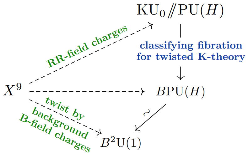
Accordingly, the generalized nonabelian cohomology theory classified by $\mathcal{A} \,\equiv\, KU_0 \sslash PU(\mathscr{H})$ decomposes over the ordinary integral cohomology in degree 3, with fibers being the abelian Whitehead-generalized cohomology of topological K-theory, and as such it may and traditionally is understood as an abelian but twisted cohomology theory: twisted topological K-theory [Atiyah & Segal 2004, Def. 3.3; Freed, Hopkins & Teleman 2007, (2.6); SS21-Bun, Ex. 4.5.4; FSS23-Char, Ex. 3.4]. Moreover, under this decomposition, the nonabelian character map on (44) is [FSS23-Char, Prop. 10.1] the twisted Chern character (the archetypical example which gives its name to the more general “character map”).

Therefore, choosing (44) as the flux quantization law for the unbounded RR-fields means to hypothesize/declare that RR-field flux and hence D-brane charge is quantized in twisted topological K-theory, with the twisted de Rham cohomology-classes of the RR-field flux densities just being the image of these K-theory classes under the twisted Chern character. This is the Hypothesis K (our terminology) originally due to Minasian & Moore 1997; and Witten 1998, with further details added by Freed & Hopkins 2000; Bouwknegt & Mathai 2001 and others.

Remark

(comparison to the literature)
The original motivation close to the above logic via the character map may be found in Witten 1998, in the paragraph wrapping p. 9-10 .

When comparing to Minasian & Moore 1997 beware that these authors, and the literature following them, take the $\mathbb{R}$-rational D-brane charge to be expressed by the Chern character multiplied with the square root of the A-hat genus of the tangent bundle of spacetime. However, since this term is multiplicatively invertible (being a unit plus a sum of inhomogeneous differential forms which are nilpotent under wedge product), this is not intrinsic to the notion of D-brane charge and may be disregarded for the purpose of charge quantization (cf. Freed & Hopkins 2000, ftn. 12); its role is rather as a technical convenience making the Chern character natural under push-forward [Brodzki, Mathai, Rosenberg & Szabo 2008, §2].

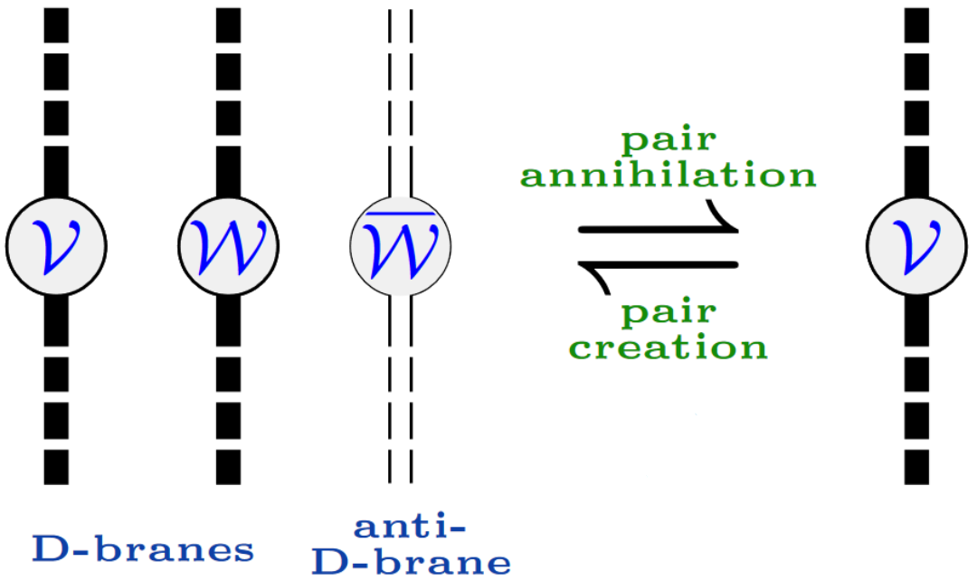
An influential argument why Hypothesis K (44) should be singled out among other compatible choices of RR-field flux quantization was the observation by Witten 1998, §3 that the equivalence relation on virtual vector bundles which characterizes topological K-theory $KU_0(X)$ on compact Hausdorff spaces (see there) plausibly mimics the expected mechanism (“Sen's conjecture”) of D-brane/anti D-brane-annihilation via tachyon condensation, by which isomorphic but opposite Chan-Paton bundles on the worldvolume of coincident D-branes should mutually annihilate.

Beware that this is a heuristic argument: There is no string-theoretic computation which actually verifies this intuition [cf. commentary by Erler 2013, p. 32]. In fact Witten 1998, ftn. 2 already points out that on closer inspection it is less clear how the picture should work.

This seems noteworthy in view of the fact that the starting point (43) of Hypothesis K is a little shaky (as discussed after Ex. ): There seems to be room to speculate that Hypothesis K will have to receive corrections. This motivates having a closer look at the flux quantization of the M-theoretic avatar of the RR-fields: The C-field.

C-Field flux quantization in 11d

Recalling the C-field‘s Gauss law (Ex. , Prop. ):

$$SolSpace \;=\; \left\{ \; \begin{array}{l} B_4 \,\in\, \Omega^4_{dR}(X^{10}) \\ B_7 \,\in\, \Omega^7_{dR}(X^{10}) \end{array} \;\;\; \text{s.t.} \;\;\; \begin{array}{rcl} \mathrm{d} \, B_4 &=& 0 \\ \mathrm{d} \, B_7 &=& -\tfrac{1}{2} B_4 \wedge B_4 \end{array} \; \right\}$$

its admissible flux quantization laws have a classifying space $\mathcal{A}$ whose $\mathbb{R}$-Sullivan algebra is as follows

$$CE(\mathfrak{l}\mathcal{A}) \;\; = \;\; \mathbb{R}\big[ b_4, b_7 \big] \Big/ \left( \begin{array}{rcl} \mathrm{d} \, b_4 &=& 0 \\ \mathrm{d} \, b_7 &=& -\tfrac{1}{2} b_4 \wedge b_4 \end{array} \right) \,.$$

We discuss now two possible choices of such flux quantization laws $\mathcal{A}$ for the C-field that have been considered in the literature (here we denote them by $\mathcal{A}_{{}_{DFM}}$ and $\mathcal{A}_{{}_{FSS}}$, respectively), both of which, while quite distinct from each other, being an “evident” choice from their respective natural perspective.

Recall again that, besides these “evident” choices, there are an infinitude of admissible variant flux quantization laws which differ in their torsion-content. In the present case, any such choice is a hypothesis/definition concerning aspects of the elusive M-theory. Careful investigation of the implications of the “evident” flux quantization laws of the C-field may not only serve to decide if either is “correct” (which is not always straightforward to decide, as long as a plausibly complete definition of M-theory remains missing), but also to understand how variant flux quantization laws would have to be chosen if the “evident” ones are deemed to have undesireable implications.

DFM flux-quantization.

If one takes the point of view that a higher $\mathrm{U}(1)$-flux quantization law as in Ex. is the most natural starting point, which naively would demand $G_4$ to be quantized in integral 4-cohomology with classifying space $B^4 \mathbb{Z} \equiv K(\mathbb{Z}, 4)$, then one is naturally led to consider the deformation of this situation which just adds-on the condition that half the cup-square of this 4-class be trivialized in rational cohomology:

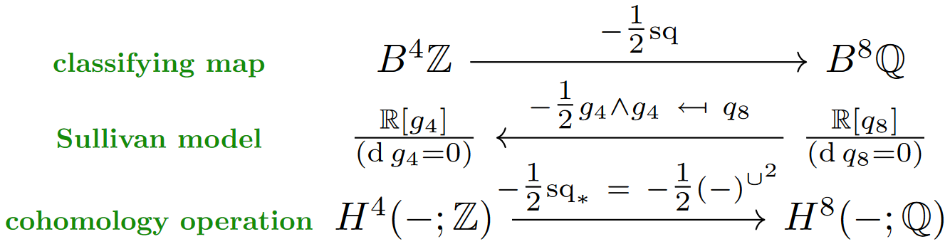
In terms of classifying spaces this means to pass to the homotopy fiber, here to be denoted $\mathcal{A}_{{}_{DFM}}$, of the map that classifies (minus) half the cup-square cohomology operation on integral 4-cohomology. This has the required Sullivan model, as shown (these kinds of computations are reviewed in FSS23-Char, §1, §5):

(45)

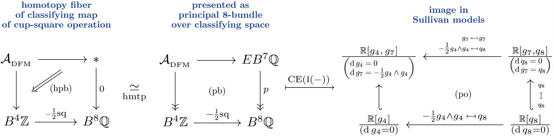
This flux quantization law is essentially that considered in Diaconescu, Freed & Moore 2003, when specialized to the case where $\tfrac{1}{2}p_1[T X^d]$ is even (the desired half-integral shift by $\tfrac{1}{2}\big(\tfrac{1}{2}p_1\big)$ is essentially added “by hand” by these authors and thus falls out of the systematics of flux quantization as discussed here).

While this DFM-model manifestly enforces quantization of charges of singular M5-branes, it is not so clear why the charge of the singular M2-branes (“Page charge”) would be quantized in this model (but see the claim by Moore 2004, §5).

FSS flux-quantization.

Another perspective is to regard the baseline of all flux quantization to be that classified by the point $\mathcal{A}_0 = \ast$ (for the entirely trivial higher gauge theory) and to obtain non-trivial classifying spaces from this maximally unbiased starting point by iterated cell attachment in the sense of CW-complexes.

The minimal choice of C-field flux quantization in this sense, requiring the minimum number 1 of cell attachments, is to take $\mathcal{A}_{{}_{FSS}} \,\equiv\, S^4$ to be the (homotopy type of) the 4-sphere (which is a valid choice of C-field flux quantization, by the examples explained above).

Since the generalized nonabelian cohomology theory classified by the (homotop types? of) n-spheres is known as Cohomotopy (being the formal dual to the “nonabelian homology theory” given by forming homotopy groups).

(…)

B-Field flux quantization in 6d

(…)

Green-Schwarz mechanicm in 10d & 6d

(…)

References

• Alexei Abrikosov, On the Magnetic properties of superconductors of the second group, Sov. Phys. JETP 5 (1957) 1174-1182; Zh. Eksp. Teor. Fiz. 32 (1957) 1442-1452 [spire:9138, pdf]

• Luigi Alfonsi, Higher geometry in physics, in: Encyclopedia of Mathematical Physics 2nd ed, Elsevier (2024) [arXiv:2312.07308]

• Orlando Alvarez, Cohomology and Field Theory, talk at: Symposium on Anomalies, Geometry, Topology, Argonne IL (28-30 March 1985) [inspire:965785, pdf, pdf]

• Orlando Alvarez, Topological quantization and cohomology, Comm. Math. Phys. 100 2 (1985) 279-309 [euclid:cmp/1103943448]

• Paolo Aschieri, Branislav Jurčo, Gerbes, M5-Brane Anomalies and $E_8$ Gauge Theory, JHEP 0410:068 (2004) [arXiv:hep-th/0409200, doi:10.1088/1126-6708/2004/10/068]

• Michael Atiyah, Graeme Segal, Twisted K-theory, Ukrainian Math. Bull. 1 3 (2004) [arXiv:math/0407054, journal page, published pdf]

• Igor Bandos, Nathan Berkovits, Dmitri Sorokin, Duality-Symmetric Eleven-Dimensional Supergravity and its Coupling to M-Branes, Nucl. Phys. B 522 (1998) 214-233 [doi:10.1016/S0550-3213(98)00102-3, arXiv:hep-th/9711055]

• Christian Becker, Marco Benini, Alexander Schenkel, Richard Szabo, Rem. 2.3 in: Abelian duality on globally hyperbolic spacetimes, Commun. Math. Phys. 349 (2017) 361-392 [arXiv:1511.00316, doi:10.1007/s00220-016-2669-9]

• Oren Bergman, Eric G. Gimon, Petr Hořava, Brane Transfer Operations and T-Duality of Non-BPS States, JHEP 9904 (1999) 010 [arXiv:hep-th/9902160, doi:10.1088/1126-6708/1999/04/010]

• Ralph Blumenhagen, Dieter Lüst, Stefan Theisen, Brane solutions in supergravity, chapter 18.5 in: Basic Concepts of String Theory, Springer (2013) [doi:10.1007/978-3-642-29497-6]

• Leron Borsten, Mehran Jalali Farahani, Branislav Jurčo, Hyungrok Kim, Jiří Nárožný, Dominik Rist, Christian Saemann, Martin Wolf, Higher Gauge Theory, in Encyclopedia of Mathematical Physics 2nd ed, Elsevier (2024) [arXiv:2401.05275]

• Peter Bouwknegt, Varghese Mathai, D-branes, B-fields and twisted K-theory, Int. J. Mod. Phys. A 16 (2001) 693-706 [arXiv:hep-th/0002023, doi:10.1088/1126-6708/2000/03/007]

• Vincent Braunack-Mayer, Hisham Sati, Urs Schreiber, Gauge enhancement of Super M-Branes, Comm. Math. Phys. 371 (2019) 197-265 [arXiv:1806.01115, doi:10.1007/s00220-019-03441-4]

• Jacek Brodzki, Varghese Mathai, Jonathan Rosenberg, Richard Szabo, D-Branes, RR-Fields and Duality on Noncommutative Manifolds, Commun. Math. Phys. 277 (2008) 643-706 [arXiv:hep-th/0607020, doi:10.1007/s00220-007-0396-y]

• Alan Carey, Stuart Johnson, Michael Murray, Holonomy on D-Branes, Journal of Geometry and Physics 52 2 (2004) 186-216 [arXiv:hep-th/0204199, doi:10.1016/j.geomphys.2004.02.008]

• Eugene Cremmer, Bernard Julia, H. Lu, Christopher Pope, Section 3 of: Dualisation of Dualities, II: Twisted self-duality of doubled fields and superdualities, Nucl. Phys. B 535(1998) 242-292 $[$arXiv:hep-th/9806106, doi:10.1016/S0550-3213(98)00552-5$]$

• Duiliu-Emanuel Diaconescu, Dan Freed, Greg Moore, The $M$-theory 3-form and $E_8$-gauge theory, in: Elliptic Cohomology Geometry, Applications, and Higher Chromatic Analogues, Cambridge University Press 2007 [arXiv:hep-th/0312069, doi:10.1017/CBO9780511721489]

• P.A.M. Dirac, Quantized Singularities in the Electromagnetic Field, Proceedings of the Royal Society A 133 (1931) 60-72 [doi:10.1098/rspa.1931.0130]

• Michael Duff, Jian Xin Lu, Black and super $p$-branes in diverse dimensions, Nucl. Phys. B 416 (1994) 301-334 [arXiv:hep-th/9306052, doi:10.1016/0550-3213(94)90586-X]

• Michael Faraday, Delienation of Lines of Magnetic Force by iron filings, §37 in: Experimental Researches in Electricity.–Twenty-Ninth Series, Philosophical Transactions of the Royal Society of London 142 (1852) 137-159 [doi:10.1098/rstl.1852.0012, jstor:108540]

  (the notion of “lines of force” is introduced on pp. 154)

• José Figueroa-O'Farrill, Joan Simón, Supersymmetric Kaluza-Klein reductions of M2 and M5-branes, Adv. Theor. Math. Phys. 6 (2003) 703-793 [arXiv:hep-th/0208107, doi:10.4310/ATMP.2002.v6.n4.a4]

• Domenico Fiorenza, Hisham Sati, Urs Schreiber, The moduli 3-stack of the C-field, Communications in Mathematical Physics 333 1 (2015) 117-151, [arXiv:1202.2455, doi:10.1007/s00220-014-2228-1]

• Domenico Fiorenza, Hisham Sati, Urs Schreiber, Rational sphere valued supercocycles in M-theory and type IIA string theory, J. Geometry and Physics, 114 (2017) 91-108 [arXiv:1606.03206, doi:10.1016/j.geomphys.2016.11.024]

• Domenico Fiorenza, Hisham Sati, Urs Schreiber, The rational higher structure of M-theory in: Proceedings of the LMS-EPSRC Durham Symposium: Higher Structures in M-Theory 2018, August 2018, Fortschritte der Physik 67 8-9 (2019) [arXiv:1903.02834, doi:10.1002/prop.201910017]

• Domenico Fiorenza, Hisham Sati, Urs Schreiber, Twisted Cohomotopy implies M-theory anomaly cancellation on 8-manifolds, Comm Math. Phys. 377 (2020) 1961-2025 [arXiv:1904.10207, doi:10.1007/s00220-020-03707-2]

• Domenico Fiorenza, Hisham Sati, Urs Schreiber, Twisted Cohomotopy implies M5 WZ term level quantization, Comm. Math. Phys. 384 (2021) 403–432 [arXiv:1906.07417, doi:10.1007/s00220-021-03951-0]

• Domenico Fiorenza, Hisham Sati, Urs Schreiber, The Character Map in Nonabelian Cohomology — Twisted, Differential, Generalized, World Scientific (2023) [arXiv:2009.11909, doi:10.1142/13422]

• Daniel Freed, Dirac charge quantization and generalized differential cohomology, Surveys in Differential Geometry 7, Int. Press (2000) 129-194 [arXiv:hep-th/0011220, doi:10.4310/SDG.2002.v7.n1.a6, spire:537392]

• Daniel Freed, Michael Hopkins, On Ramond-Ramond fields and K-theory, JHEP 0005 (2000) 044 $[$arXiv:hep-th/0002027, doi:10.1088/1126-6708/2000/05/044$]$

• Daniel S. Freed, Michael Hopkins, Constantin Teleman, Twisted equivariant K-theory with complex coefficients, Journal of Topology 1 1 (2007) [arXiv:math/0206257, doi:10.1112/jtopol/jtm001]

• Daniel S. Freed, Gregory W. Moore, Graeme Segal, The Uncertainty of Fluxes, Commun. Math. Phys. 271 (2007) 247-274 [arXiv:hep-th/0605198, doi:10.1007/s00220-006-0181-3]

• Daniel S. Freed, Gregory W. Moore, Graeme Segal, Heisenberg Groups and Noncommutative Fluxes, Annals Phys. 322 (2007) 236-285 [arXiv:hep-th/0605200, doi:10.1016/j.aop.2006.07.014]

• Daniel Freed, Edward Witten, Anomalies in String Theory with D-Branes, Asian J. Math. 3 4 (1999) 819-852 [arXiv:hep-th/9907189, InSpire:2655986]

• Krzysztof Gawędzki, Topological Actions in two-dimensional Quantum Field Theories, in: Nonperturbative quantum field theory, Nato Science Series B 185, Springer (1988) [spire:257658, doi:10.1007/978-1-4613-0729-7_5, pdf]

• Krzysztof Gawędzki, Nuno Reis, WZW branes and gerbes, Rev. Math. Phys. 14 (2002) 1281-1334 [arXiv:hep-th/0205233, doi:10.1142/S0129055X02001557]

• Grigorios Giotopoulos, Hisham Sati: Smooth Sets of Fields [arXiv:2312.16301]

• Marc Henneaux, Claudio Teitelboim, Quantization of Gauge Systems, Princeton University Press (1992) [doi:10.2307/j.ctv10crg0r]

• Michael Hopkins, Isadore Singer, Quadratic Functions in Geometry, Topology, and M-Theory, J. Differential Geom. 70 3 (2005) 329-452 [arXiv:math.AT/0211216, doi:10.4310/jdg/1143642908, euclid:1143642908]

• Hyperphysics, Magnetic Flux [hyperphysics.phy-astr.gsu.edu/hbase/magnetic/fluxmg.html]

• Calin Lazaroiu, Carlos S. Shahbazi, around Def. 1.16 in: The duality covariant geometry and DSZ quantization of abelian gauge theory, Advances in Theoretical and Mathematical Physics 26 (2022) 2213–2312 [arXiv:2101.07236, doi:10.4310/ATMP.2022.v26.n7.a5]

• Calin Lazaroiu, Carlos S. Shahbazi, around (3) in: The geometry and DSZ quantization of four-dimensional supergravity, Letters in Mathematical Physics 113 4 (2023) [arXiv:2101.07778, doi:10.1007/s11005-022-01626-y]

• J. C. Loudon, P. A. Midgley, Imaging Flux Vortices in Type II Superconductors with a Commercial Transmission Electron Microscope, Ultramicroscopy 109 6 (2009) 700-729 [arXiv:0807.2401, doi:10.1016/j.ultramic.2009.01.008]

• Thomas Martin (ed.), Faraday’s diary of experimental investigation 1820-1862, HR Direct (2009) [webpage, preview:pdf]

• Karapet Mkrtchyan, Fridrich Valach, Democratic actions for type II supergravities, Phys. Rev. D 107 6 (2023) 066027 [doi:10.1103/PhysRevD.107.066027arXiv:2207.00626]

• Greg Moore, Anomalies, Gauss laws, and Page charges in M-theory, Comptes Rendus Physique 6 (2005) 251-259 [arXiv:hep-th/0409158, doi:10.1016/j.crhy.2004.12.005]

• Joseph Polchinski, Dirichlet-Branes and Ramond-Ramond Charges, Phys. Rev. Lett. 75 (1995) 4724-4727 [arXiv:hep-th/9510017, doi:10.1103/PhysRevLett.75.4724]

• Ruben Minasian, Gregory Moore, K-theory and Ramond-Ramond charge, JHEP 9711:002 (1997) [arXiv:hep-th/9710230, doi:10.1088/1126-6708/1997/11/002]

• Hisham Sati, Geometric and topological structures related to M-branes, in Superstrings, Geometry, Topology, and $C^\ast$-algebras, Proc. Symp. Pure Math. 81 (2010) 181-236 [arXiv:1001.5020, ams:pspum/081]

• Hisham Sati, Urs Schreiber, Equivariant principal $\infty$-bundles [arXiv:2112.13654]

• Hisham Sati, Urs Schreiber, M/F-Theory as $M f$-Theory, Rev. Math. Phys. 35 10 (2023) [doi:10.1142/S0129055X23500289, arXiv:2103.01877]

• Hisham Sati, Urs Schreiber, Flux Quantization on Phase Space [arXiv:2312.12517]

• Hisham Sati, Urs Schreiber, Quantum Observables of Quantized Fluxes [arXiv:2312.13037]

• Hisham Sati, Alexander Voronov, (13) in: Mysterious Triality and M-Theory [arXiv:2212.13968]

• Urs Schreiber, Higher Topos Theory in Physics, in Encyclopedia of Mathematical Physics 2nd ed, Elsevier (2024) [arXiv:2311.11026]

• Edward Witten, On Flux Quantization In M-Theory And The Effective Action, J. Geom. Phys. 22 1 (1997) 1-13 [arXiv:hep-th/9609122, doi:10.1016/S0393-0440(96)00042-3]

• Edward Witten, D-Branes And K-Theory, JHEP 9812:019 (1998) [arXiv:hep-th/9810188, doi:10.1088/1126-6708/1998/12/019]

(…)