nLab photon propagator
Context
Algebraic Qunantum Field Theory
algebraic quantum field theory (perturbative, on curved spacetimes, homotopical)
Concepts
quantum mechanical system, quantum probability
interacting field quantization
Theorems
States and observables
Operator algebra
Local QFT
Perturbative QFT
Fields and quanta
fields and particles in particle physics
and in the standard model of particle physics:
matter field fermions (spinors, Dirac fields)
| flavors of fundamental fermions in the standard model of particle physics: | |||
|---|---|---|---|
| generation of fermions | 1st generation | 2nd generation | 3d generation |
| quarks () | |||
| up-type | up quark () | charm quark () | top quark () |
| down-type | down quark () | strange quark () | bottom quark () |
| leptons | |||
| charged | electron | muon | tauon |
| neutral | electron neutrino | muon neutrino | tau neutrino |
| bound states: | |||
| mesons | light mesons: pion () ρ-meson () ω-meson () f1-meson a1-meson | strange-mesons: ϕ-meson (), kaon, K*-meson (, ) eta-meson () charmed heavy mesons: D-meson (, , ) J/ψ-meson () | bottom heavy mesons: B-meson () ϒ-meson () |
| baryons | nucleons: proton neutron |
(also: antiparticles)
hadrons (bound states of the above quarks)
minimally extended supersymmetric standard model
bosinos:
dark matter candidates
Exotica
Contents
Idea
Considering the Lagrangian field theory of the free field theory electromagnetic field, the corresponding Feynman propagator describes the time-ordered product of linear observables of the vector potential and may be thought of as the probability amplitude for a photon to travel from to . Therefore this is often called the photon propagator.
For details see at A first idea of quantum field theory this prop..
Example
(Feynman amplitudes in causal perturbation theory – example of QED)
In perturbative quantum field theory, Feynman diagrams are labeled multigraphs that encode products of Feynman propagators, called Feynman amplitudes (this prop.) which in turn contribute to probability amplitudes for physical scattering processes – scattering amplitudes:
The Feynman amplitudes are the summands in the Feynman perturbation series-expansion of the scattering matrix
of a given interaction Lagrangian density .
The Feynman amplitudes are the summands in an expansion of the time-ordered products of the interaction with itself, which, away from coincident vertices, is given by the star product of the Feynman propagator (this prop.), via the exponential contraction
Each edge in a Feynman diagram corresponds to a factor of a Feynman propagator in , being a distribution of two variables; and each vertex corresponds to a factor of the interaction Lagrangian density at .
For example quantum electrodynamics in Gaussian-averaged Lorenz gauge involves (via this example):
-
the Dirac field modelling the electron, with Feynman propagator called the electron propagator (this def.), here to be denoted
-
the electromagnetic field modelling the photon, with Feynman propagator called the photon propagator (this prop.), here to be denoted
The Feynman diagram for the electron-photon interaction alone is
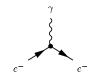
where the solid lines correspond to the electron, and the wiggly line to the photon. The corresponding product of distributions is (written in generalized function-notation)
Hence a typical Feynman diagram in the QED Feynman perturbation series induced by this electron-photon interaction looks as follows:
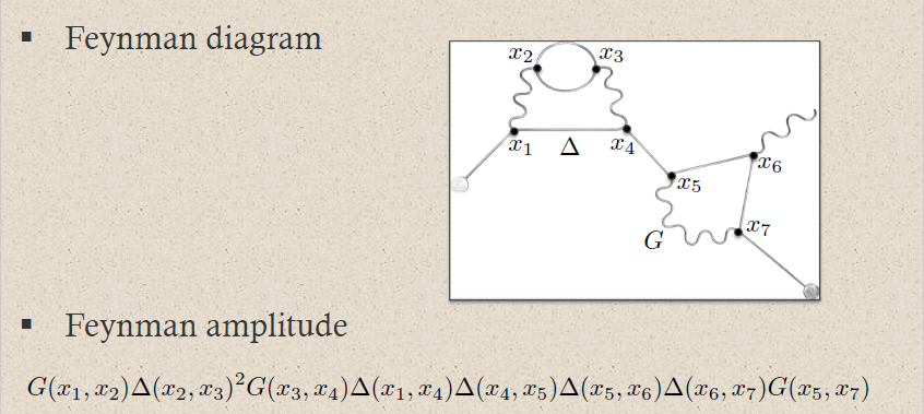
where on the bottom the corresponding Feynman amplitude product of distributions is shown; now notationally suppressing the contraction of the internal indices and all prefactors.
For instance the two solid edges between the vertices and correspond to the two factors of :
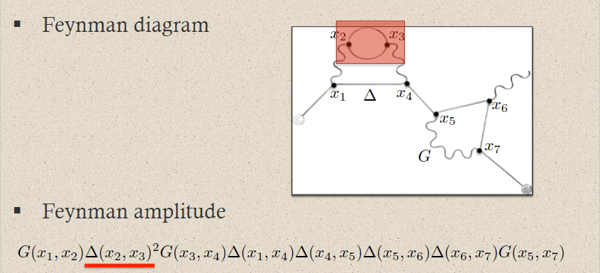
This way each sub-graph encodes its corresponding subset of factors in the Feynman amplitude:
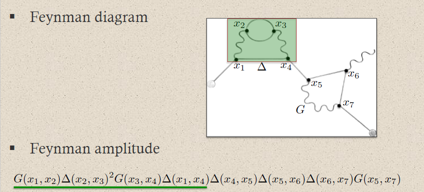
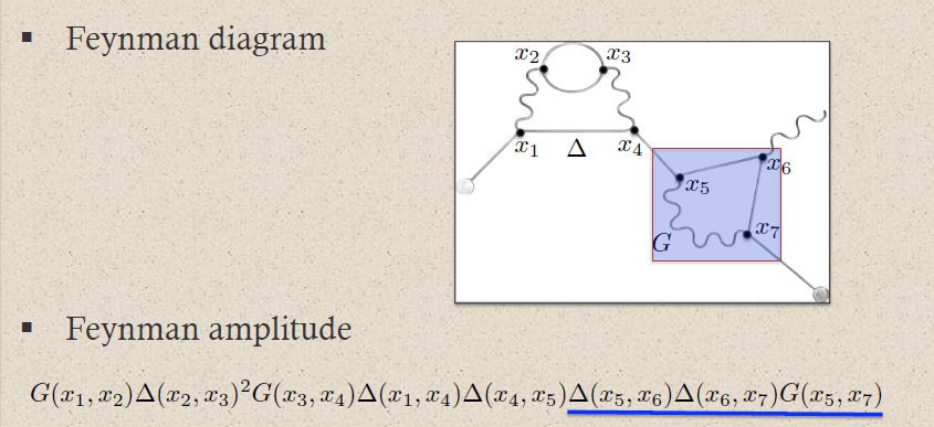
graphics grabbed from Brouder 10
A priori this product of distributions is defined away from coincident vertices: . The definition at coincident vertices requires a choice of extension of distributions to the diagonal locus. This choice is the ("re-")normalization of the Feynman amplitude.
Related concepts
References
- Radovan Dermisek, Quantum Electrodynamics (QED) (pdf, pdf)
Last revised on January 20, 2018 at 16:24:45. See the history of this page for a list of all contributions to it.