nLab microcausal polynomial observable
Context
Algebraic Quantum Field Theory
algebraic quantum field theory (perturbative, on curved spacetimes, homotopical)
Concepts
quantum mechanical system, quantum probability
interacting field quantization
Theorems
States and observables
Operator algebra
Local QFT
Perturbative QFT
Functional analysis
Overview diagrams
Basic concepts
Theorems
Topics in Functional Analysis
Contents
Idea
The microcausal functionals on the space of smooth functions on a globally hyperbolic spacetime are those which come from compactly supported distributions on some Cartesian product of copies of such that the wave front set of the distributions excludes those covectors to a point in all whose components are in the closed future cone or all whose components are in the closed past cone
These functionals underly the Wick algebra of free field theories. The condition on the wave front is such that the product of distributions with a Hadamard distribution is well defined, so that the coresponding Moyal star product is well defined, which gives the Wick algebra. At the same time the condition includes local observables and hence in particular the usual (adiabatically switched) point-interaction terms, such as of phi^4 theory.
Definition
Definition
Let be field bundle which is a vector bundle. An off-shell polynomial observable is a smooth function
on the on-shell space of sections of the field bundle (space of field histories) which may be expressed as
where
is a compactly supported distribution of k variables on the -fold graded-symmetric external tensor product of vector bundles of the field bundle with itself.
Write
for the subspace of off-shell polynomial observables onside all off-shell observables.
Let moreover be a free Lagrangian field theory whose equations of motion are Green hyperbolic differential equations. Then an on-shell polynomial observable is the restriction of an off-shell polynomial observable along the inclusion of the on-shell space of field histories . Write
for the subspace of all on-shell polynomial observables inside all on-shell observables.
By this prop. restriction yields an isomorphism between polynomial on-shell observables and polynomial off-shell observables modulo the image of the differential operator :
Definition
For a spacetime, hence a Lorentzian manifold with time orientation, then a microcausal observable is a polynomial observable (def. ) such that each coefficient has wave front set excluding those points where all wave vectors are in the closed future cone or all in the closed past cone.
Examples
Example
(non-singular observables are microcausal)
Let be a free Lagrangian field theory.
Then a regular observable, hence a polynomial observable (this def.) whose distributional coefficients (?) are non-singular distributions is a microcausal observable (def. ).
This is simply because the wave front set of non-singular distributions is empty (by definition, via the Paley-Wiener-Schwartz theorem, this prop.).
Example
(compactly averaged point evaluations are microcausal)
Let be a free Lagrangian field theory. Assume the field bundle is a trivial vector bundle with linear fiber coordinates .
Let be a bump function, then for the polynomial observables (this def.) of the form
are microcausal (def. ).
If here we think of as a point-interaction term (as for instance in phi^4 theory) then is to be thought of as an “adiabatically switched” coupling constant. These are the relevant interaction terms to be quantized via causal perturbation theory.
Proof
For notational convenience, consider the case of the scalar field with ; the general case is directly analogous. Then the local observable coming from (a phi^n interaction-term), has, regarded as a polynomial observable, the delta distribution as coefficient in degree 2:
Now for and a chart around this point, the Fourier transform of distributions of restricted to this chart is proportional to the Fourier transform of evaluated at the sum of the two covectors:
Since is a plain bump function, its Fourier transform is quickly decaying (according to this inequality) along (this prop.), as long as . Only on the cone the Fourier transform is constant, and hence in particular not decaying.
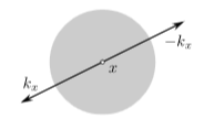
This means that the wave front set consists of the elements of the form with . Since and are both in the closed future cone or both in the closed past cone precisely if , this situation is excluded in the wave front set and hence the distribution is microcausal.
(graphics grabbed from Khavkine-Moretti 14, p. 45)
This shows that microcausality in this case is related to conservation of momentum in the point interaction.
More generally:
Example
(polynomial local observables are microcausal)
Write
for the space of differential forms on the jet bundle of the field bundle which locally are polynomials in the field variables.
for the subspace of horizontal differential forms of degree on the jet bundle (local Lagrangian densities) of those which are compactly supported with respect to (local observables) and polynomial with respect to the field variables.
Every induces a functional
by integration of the pullback of along the jet prolongation of a given section:
These functionals happen to be microcausal, so that there is an inclusion
into the space of microcausal functionals (e.g. Fredenhagen-Rejzner 12, p. 21). In fact this is a dense subspace inclusion (e.g. Fredenhagen-Rejzner 12, p. 23)
Properties
Proposition
Write for that subalgebra of the algebra of microcausal functionals whose coefficients are non-singular distributions.
Let
be a state on regular observables which is quasi-free Hadamard. Then this uniquely extends to a state on microcausal functionsal
(Hollands-Ruan 01, remark 1 on p. 12, implied by Brunetti-Fredenhagen 00, Hollands-Wald 01, a special case of Hollands-Ruan 01, theorem III.1 (ii))
Related concepts
References
Original articles
-
Romeo Brunetti, Klaus Fredenhagen, Microlocal Analysis and Interacting Quantum Field Theories: Renormalization on Physical Backgrounds, Commun. Math. Phys. 208 : 623-661, 2000 (math-ph/9903028)
-
Michael Dütsch, Klaus Fredenhagen, Algebraic Quantum Field Theory, Perturbation Theory, and the Loop Expansion, Commun.Math.Phys. 219 (2001) 5-30 (arXiv:hep-th/0001129)
-
Stefan Hollands, Robert Wald, Local Wick polynomials and time ordered products of quantum fields in curved spacetime, Commun. Math. Phys., Commun.Math.Phys.223:289-326,2001 (arXiv:gr-qc/0103074)
-
Michael Dütsch, Klaus Fredenhagen, Perturbative algebraic field theory, and deformation quantization, in Roberto Longo (ed.), Mathematical Physics in Mathematics and Physics, Quantum and Operator Algebraic Aspects, volume 30 of Fields Institute Communications, pages 151–160. American Mathematical Society, 2001
-
Stefan Hollands, Weihua Ruan, The State Space of Perturbative Quantum Field Theory in Curved Spacetimes, Annales Henri Poincare 3 (2002) 635-657 (arXiv:gr-qc/0108032)
-
Romeo Brunetti, Klaus Fredenhagen, Pedro Lauridsen Ribeiro, section 4.1 of Algebraic Structure of Classical Field Theory: Kinematics and Linearized Dynamics for Real Scalar Fields (arXiv:1209.2148)
Review
-
Klaus Fredenhagen, Katarzyna Rejzner, Perturbative algebraic quantum field theory, In Mathematical Aspects of Quantum Field Theories, Springer 2016 (arXiv:1208.1428)
-
Igor Khavkine, Valter Moretti, Algebraic QFT in Curved Spacetime and quasifree Hadamard states: an introduction, Chapter 5 in Romeo Brunetti et al. (eds.) Advances in Algebraic Quantum Field Theory, Springer, 2015 (arXiv:1412.5945)
-
Katarzyna Rejzner, section 4.4.1 of Perturbative Algebraic Quantum Field Theory, Mathematical Physics Studies, Springer 2016 (web)
-
Michael Dütsch, def. 1.2 and equation (2.47) in From classical field theory to perturbative quantum field theory, 2018
Last revised on June 11, 2022 at 10:58:58. See the history of this page for a list of all contributions to it.