Redirected from "extension of Lie algebras".
Contents
Abstract. Twisted cohomology is maps in the tangent homotopy theory of parameterized spectra. Its rationalization has a Quillen-Sullivan-type model in terms of unbounded L-∞ algebras (SS 17). Interesting examples appear by constructing iterated maximal higher central extensions of super L-∞ algebras, invariant with respect to automorphisms modulo R-symmetries – a super-equivariant version of the Whitehead tower. Applied to the superpoint, this process turns out to discover all the twisted cohomology seen in string/M-theory (FSS 13, HS 17), rationally, in particular twisted topological K-theory with 5-brane correction and with supersymmetric Chern-forms on 10d-superspace (FSS 16a). Passage to cyclic L-∞ cohomology reflects double dimensional reduction of super p-branes. Applied to twisted K-theory on 10d superspace this yields two L-∞ cocycles on 9d superspace which both classify the tangent complex of super T-folds. There appears a super L-∞ equivalence between them exhibiting supersymmetric topological T-duality, rationally (FSS 16b).
These rational phenomena indicate that integrally the super-equivariant Whitehead tower of the superpoint is a mechanism for discovering interesting twisted super-differential cohomology theories (dcct). We close with an outlook on the relevant constructions.
Lecture notes with more details are here:
Related talks
Contents
Super
For the bulk of this talk, the homotopy theory we consider
is that of super L-∞ algebras:
Those of finite type are equivalently
the formal duals
of augmented dg-algebra structures
on free -bi-graded commutative algebras
over chain complexes of super vector spaces,
namely their Chevalley-Eilenberg algebras:
We will keep using the following fact:
Proposition
(FSS 13, theorem 3.8)
Write
for the line Lie (p+2)-algebra, given by
A -cocycle on an -algebra is equivalently a super -homomorphism
The homotopy fiber of this map
is given, up to equivalence, by adjoining to a single generator
forced to be a potential for :
Example
The homotopy fiber of a 2-cocycle
is the classical central extension
that it classifies.
Hence:
The higher central extensions
classified by higher cocycles
are their homotopy fibers.
Proposition
(-Algebra and Rational homotopy theory)
L-∞ algebras capture a broad range of aspects
of rational homotopy theory:
1) The rational homotopy theory of simply connected topological spaces embeds
as the homotopy theory of connected -algebras (Quillen 69, Hinich 98):
2) The rational stable homotopy theory of rational spectra embeds
as the abelian -algebras: the plain chain complexes (Schwede-Shipley 03):
3) The parameterized homotopy theory, of rational parameterized spectra
over some connected rational space
embeds into the slice over
on those whose augmentation ideal is a chain complex (Schlegel-Schreiber):
4) Hence super L-∞ algebras generalize all this
to the rationalization of “super-homotopy theory”.
We say more about this below.
Example
(the single source of all following examples)
The simplest non-trivial super L-∞ algebras
are the superpoints
defined by
In the following we do nothing but analyzing the
consecutive higher invariant central extensions
of the superpoint.
Spacetime
Proposition
The maximal central extension of the superpoint
is the super Lie algebra
called the super-worldline of the superparticle:
-
whose even part is spanned by one generator
-
whose odd part is spanned by one generator
-
the only non-trivial bracket is
Next, the maximal central extension of
is the , super Minkowski spacetime
-
whose even part is , spanned by generators
-
whose odd part is , regarded as
the Majorana spinor representation
of
-
the only non-trivial bracket is the spinor bilinear pairing
where is the charge conjugation matrix
(and we use Einstein summation convention and leaves sums over repeated indices implicit).
Proof
(skip proof)
Recall that
-dimensional central extensions of super Lie algebras
are classified by 2-cocycles.
These are super-skew symmetric bilinear maps
satisfying a cocycle condition.
The extension that this classifies
has underlying super vector space
the direct sum
an the new super Lie bracket is given
on pairs
by
The condition that the new bracket satisfies the super Jacobi identity
is equivalent to the cocycle condition on .
Now
in the case that ,
then the cocycle condition is trivial
and a 2-cocycle is just a symmetric bilinear form
on the fermionic dimensions.
So
in the case
there is a unique such, up to scale, namely
But
in the case
there is a 3-dimensional space of 2-cocycles, namely
If this is identified with the three coordinates
of 3d Minkowski spacetime
then the pairing is the claimed one
(see at supersymmetry – in dimensions 3,4,6,10).
This phenomenon continues:
Definition
Given a super Lie algebra , write
-
for the even part of its super Lie algebra of even derivations;
-
for the stabilizer of the even part
– called the infinitesimal R-symmetries.
-
the external automorphisms, making a short exact sequence
If that sequence splits and if is reductive
then we consider the semisimple direct summand
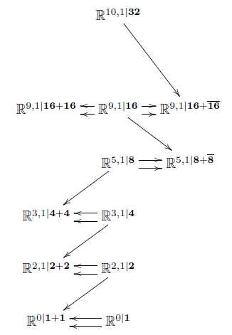
Theorem
(Huerta-Schreiber 17)
The diagram of super Lie algebras shown on the right
is obtained by consecutively forming
maximal central extensions
invariant with respect to
the semisimple external automorphisms (def. )
at the given stage.
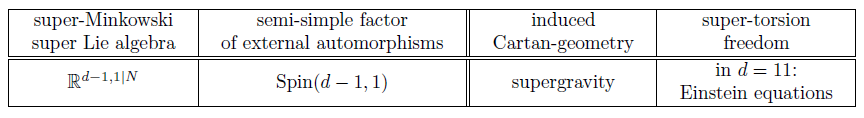
Here
is the -dimensional, -supersymmetric
super-translation algebra (see at geometry of physics – supersymmetry).
And these semisimple subgroups are in each case
the spin group covers
of the proper orthochronous Lorentz groups .
Conclusion:
Just from studying iterated invariant central extensions
of super Lie algebras,
starting with the superpoint,
we (re-)discover
-
Lorentzian geometry,
-
spin geometry.
-
super spacetimes.
May we extend further?
Branes
Proposition
(Achúcarro-Evans-Townsend-Wiltshire 87, Brandt 12-13)
The space of maximal invariant indecomposable cocycles
-
on 10d super Minkowski spacetime
is spanned by a single 3-cocycle
-
on 11d super Minkowski spacetime is spanned by the 4-cocycle
This classification is also known as
the old brane scan.
Definition
Name the homotopy fibers of these cocycles
as follows
By prop.
the superstring super Lie 2-algebra is given by
The membrane super Lie 3-algebra is given by
This dg-algebra was first considered in D’Auria-Fré 82 (3.15)
as a tool for constructing 11-dimensional supergravity.
Hence the progression
of maximal invariant extensions of the superpoint
continues as a diagram
of super L-∞ algebras like so:
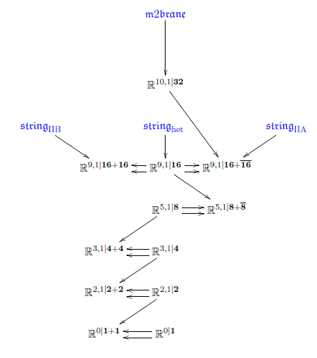
(While every extension displayed is a maximal invariant higher central extension, not all invariant higher central extensions are displayed. For instance there are string and membrane cocycles also on the lower dimensional super-Minkowski spacetimes (“non-critical”), e.g. the super 1-brane in 3d and the super 2-brane in 4d.)
The progression of invariant higher central extensions continues:
Proposition
(D’Auria-Fré 82, (3.27, 3.28))
The space of indecomposable invariant higher cocylces on is spanned by
where is the extra generator of .
Proposition
(Chryssomalakos-Azcárraga-Izquierdo-Bueno 99, Sakaguchi 99)
Define the following elements in :
Write
for their sum.
Then the indecomposable invariant cocycles on are spanned by
where is the extra generator of .
Similarly define the following elements in
Then the indecomposable invariant cocycles on are spanned by
As above, these cocycles classify
further higher super -algebra extensions
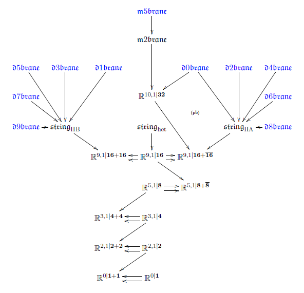
In conclusion:
by forming
iterated (maximal) invariant higher central super -extensions
of the superpoint,
we obtain the following brane bouquet-diagram:
Fields
Now given one stage in the brane bouquet
we want to descend to .
By the general theory of principal ∞-bundles (Nikolaus-Schreiber-Stevenson 12):
-
has a -∞-action
-
equipping with an -∞-action
is equivalent to finding a homotopy fiber sequence as on the right here:
-
is -equivariant precisely if it descends to a morphism
such that this diagram commutes up to homotopy:
-
if so, then resulting triangle diagram
exhibits as a cocycle in (rational) -twisted cohomology
with respect to the local coefficient bundle .
We now work out this general prescription
for the cocycles in the brane bouquet.
RR-fields
By the brane bouquet above
the type IIA D-branes
are given by super cocycles of the form
for .
Notice that
has one generator in each even degree, the universal Chern classes.
Hence the -algebra
is given by
This allows to unify the D-brane cocycles
into a single morphism of super -algebras of the form
By the above prescription, descending is equivalent
to finding a commuting diagram in the homotopy category of super -algebras
of the form
This turns out to exist as follows (Fiorenza-Sati-Schreiber 16a, section 5):
Definition
Following prop. define the -algebra
by
Moreover write
for the super -algebra whose Chevalley-Eilenberg algebra is
Proposition
(Fiorenza-Sati-Schreiber 16a, theorem 4.16)
The super -algebra
is a resolution of type IIA super-Minkowski spacetime.
in that there is a weak equivalence
This fits into a commuting diagram of the form
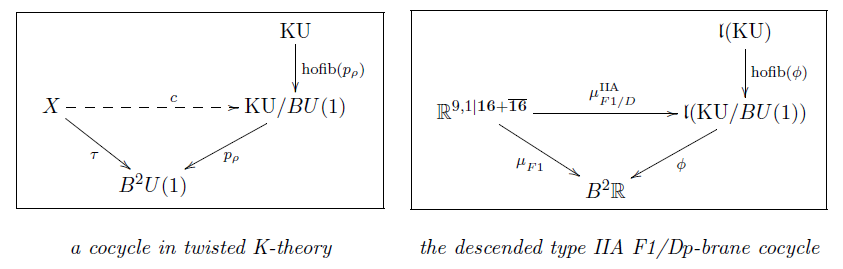
In conclusion
the type IIA F1-brane and D-brane cocycles with -coefficients
do descend to super-Minkowski spacetime
as one single cocycle with coefficients
in rationalized twisted K-theory.
M-flux fields
(skip)
The part of the brane bouquet giving the M-branes is
In order to descend this, consider the -algebra corresponding to the 4-sphere
By standard facts on rational n-spheres, this is given by
Proposition
(Fiorenza-Sati-Schreiber 15, section 3)
There is a homotopy fiber sequence of -algebras as on the right
which is the image under of the quaternionic Hopf fibration.
This makes a commuting diagram
in the homotopy category of super -algebas
of the form
In conclusion
this says that, rationally,
M2-brane charge is in degree-4 ordinary cohomology
and it twists M5-brane charge
which is, rationally, in unstable degree-4 cohomotopy.
Now that we have found
the descended -cocycles
for all super -branes
in twisted cohomology, rationally,
we may analyze their behaviour under double dimensional reduction
and discover the super -algebraic incarnation
of various dualities in string theory.
Reduction
We have discovered higher cocycles
on higher dimensional super-spacetimes.
Now we discuss that there is double dimensional reduction
which takes these to lower-degree cocycle on lower-dimensional space.
This is given by passage to cyclic loop spaces:
Proposition
Let be any (∞,1)-topos
such as
and let be an ∞-group in ,
then right base change along is a pair of adjoint ∞-functors of the form
where
∞-action for equipped with its canonical ∞-action by left multiplication and the argument
regarded as equipped with its trivial --action;
for the circle group, then this is the cyclic loop space .
Hence for
then there is a natural equivalence
given by
Proof
(skip proof)
First observe that the conjugation action on is the internal hom in the (∞,1)-category of -∞-actions . Under the equivalence of (∞,1)-categories
(from Nikolaus-Schreiber-Stevenson 12) then with its canonical ∞-action is and with the trivial action is .
Hence
Actually, this is the very definition of what is to mean in the first place, abstractly.
But now since the slice (∞,1)-topos is itself cartesian closed, via
it is immediate that there is the following sequence of natural equivalences
Here denotes the terminal morphism and denotes the base change along it.
We now apply this general mechanism to the brane bouquet.
By the discussion of rational homotopy theory above
we may think of L-∞ algebras as rational topological spaces
and more generally as rational parameterized spectra.
For instance above we found that the coefficient space
for RR-fields in rational twisted K-theory is the
L-∞ algebra.
Hence in order to apply double dimensional reduction
to super p-branes
we now specialize the above formalization to
cyclification of super L-∞ algebras (FSS 16b)
Definition
For any super L-∞ algebra of finite type, its cyclification
is defined by having Chevalley-Eilenberg algebra of the form
where
is a copy of with cohomological degrees shifted down by one, and where is a new generator in degree 2.
The differential is given for by
where on the right we are extendng as a graded derivation.
Define
in the same way, but with .
For every there is a homotopy fiber sequence
which hence exhibits as the homotopy quotient of by an -action.
The following says that the -cyclification from prop.
indeed does model correspond to the topological cyclification .
Proposition
(Vigué-Sullivan 76, Vigué-Burghelea 85)
If
is the -algebra associated by rational homotopy theory to a simply connected topological space ,
then its cyclification (def. )
corresponds to the cyclic loop space of
The cochain cohomology of the Chevalley-Eilenberg algebra
computes the cyclic cohomology of with coefficients in .
Moreover the homotopy fiber sequence of the cyclification corresponds to that of the free loop space:
We now have the following super -algebraic incarnation
of the general double dimensional reduction from prop. :
Proposition
(Fiorenza-Sati-Schreiber 16b, prop. 3.5)
Let
be a central extension of super L-∞ algebras. According to prop. we have
and hence every generator has a unique decomposition
where and do not involve the generator . We may think of this as
Under this identification any super -homomorphism
hence a dg-algebra homomorphism
gives rise to a homomorphism of the form
which, in the notation of def. , is given dually by
Moreover, this construction constitutes a natural bijection
between super -homomorphisms out of the exteded super -algebra and homomorphism out of the base into the cyclification (def. ) of the original coefficients with the latter constrained so that the canonical 2-cocycle on the cyclification is taken to the 2-cocycle classifying the given extension.
Example
(skip example)
Let
be the extension of a super Minkowski spacetime from dimension to dimension .
Let moreover
be the line Lie (p+3)-algebra
and consider any super (p+1)-brane cocycle from the old brane scan in dimension
Then the cyclification of the coefficients (prop. ) is
and the dimensionally reduced cocycle
has the following components
It follows that with
also
This is the dimensional reduction observed in the old brane scan (Achúcarro-Evans-Townsend-Wiltshire 87)
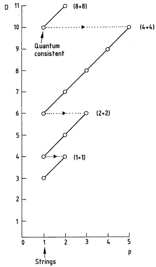
graphics grabbed from (Duff 87)
But there is more: the un-wrapped component of the dimensionally reduced cocycle satisfies the twisted cocycle condition
These relations are not to be ignored.
This we turn to now.
T-Duality
We consider now the D-brane cocycles
on type IIA and IIB superspacetime
and dimensionally reduce both to their joint 9d base space.
There we discover a hidden duality: T-duality.
Proposition
(Fiorenza-Sati-Schreiber 16b, prop. 5.1)
The cyclification (def. ) of (def. ) has CE-algebra
The cyclification of has CE-algebra
Hence there is an -isomorphism of the form
relating the cyclifications of the rational twisted KU-coefficients, which is given by
Proof
(skip proof)
By def. , as a polynomial algebra the CE-algebra of is obtained from the CE-algebra of by adding a shifted copy of each generator. We denote by the shifted copy of and by the shifted copy of . The differential is then defined by
Next, again by def. , the CE-algebra of is obtained by adding a further degree 2 generator and defining the differential as
The proof for is completely analogous.
Hence postcomposition with
sends the doubly dimensionally reduced IIA/B D-brane cocycles
to some other super -cocycles.
The following theorem says that
indeed it takes them into each other:
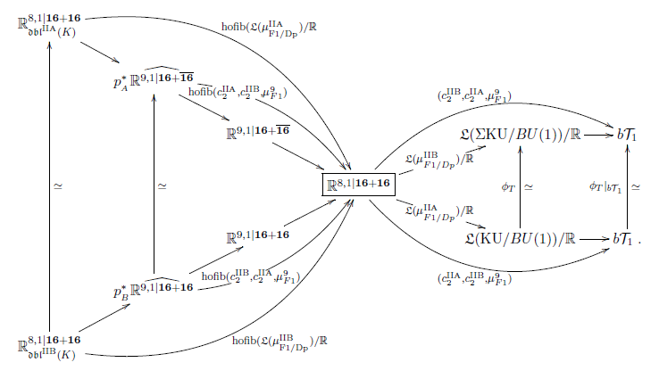
Theorem
(Fiorenza-Sati-Schreiber 16b, theorem 5.3)
The following diagram commutes
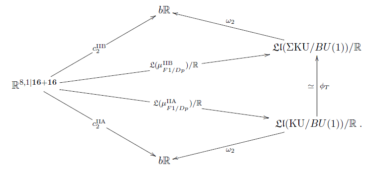
In particular this means that
-
.
-
.
The first of these two conditions is
the super -version of the axiom for
topological T-duality due to Bouwknegt-Evslin-Mathai 04.
To understand the second condition
pass to the correspondence super -algebra.
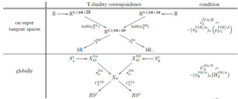
Proposition
(Fiorenza-Sati-Schreiber 16b, prop. 6.2)
We have a diagram of super -algebras of the following form
such that on the classifying 3-cocycles
is given by the Poincaré form
as
This now is the super -version of the
refined formulation of topological T-duality
due to Bunke-Schick 04:
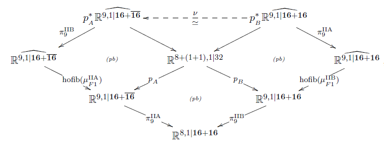
Proposition
(Fiorenza-Sati-Schreiber 16b, prop. 6.4)
The integral transform of pull-push through this correspondence is an isomorphism
Moreover, it identifies the type IIA D-brane cocycles with those of type IIB (from def. ), as in Theorem :
Proof
One checks that
With this the statement follows from theorem , item 2.
Prop. is the super -algebraic analog of Bunke-Schick 04, theorem 3.13.
In fact on CE-algebras this is the Buscher rules for RR-fields
also known as Hori’s formula (Hori 99).
To see why the above correspondence
follows from the double dimensional reduction isomorphism
it is useful to break up the doubly dimensionally reduced cocycles
into the part for the fiber bundle and the part for the K-cocycles:
Definition
The delooped T-duality Lie 2-algebra
is the homotopy fiber of the cup square of the first Chern class
hence by prop.
Proposition
(FSS 16b, prop. 7.3)
The dimensionally reduced twisted K-theory coefficients from prop.
sit in a homotopy fiber sequence of the form
exhibiting (via NSS 12) an ∞-action
of the T-duality Lie 2-algebra from def.
on .
Proposition
(FSS 16b, prop. 7.5)
The homotopy fiber of the cyclified IIA/B cocycles (theorem )
projected to the T-duality Lie 2-algebra (def. )
are the super -algeberas and from prop.
hence the Bunke-Schick 04-type correspondence
follows from theorem
via -functoriality of homotopy fibers:
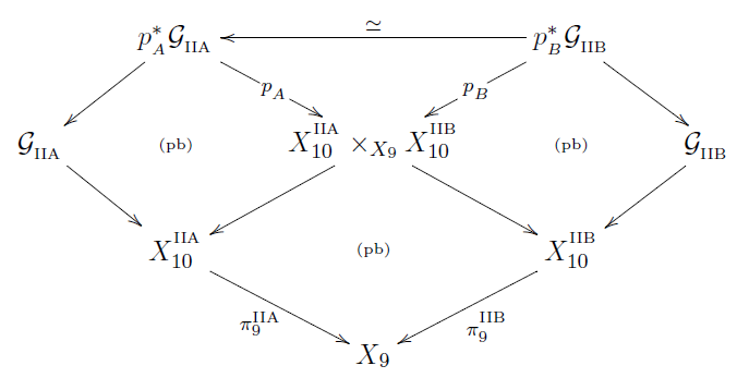
Prop. implies that we may study T-duality
in terms of principal 2-bundles for the T-duality 2-group
over 9d super-manifolds locally modeled on .
This is the supergeometric refinement
of the 2-bundle perspective on T-folds due to (Nikolaus 14).
Integral lift
The above super -algebra
is to be the curvature/Chern character data
of twisted differential cohomology
on supermanifolds.
Consider the (∞,1)-topos over the site of all super-formal manifolds
Hence is a “super formal smooth ∞-groupoid”.
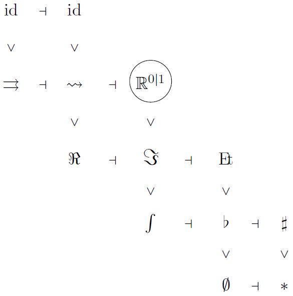
In conclusion
this progression of adjoint modalities
is the abstract reflection that inside
there is a good theory of
-
differential cohomology
-
differential geometry
-
supergeometry
Regarding the first point:
The fracture squares
exhibit each as a differential cohomology theory (Bunke-Nikolaus-Völkl 13)
(the differential cohomology hexagon).
In particular if
the non-differential twisted generalized cohomology theory is prescribed
then a differential refinement is obtained by
setting:
where denotes the sheaf of flat super L-∞ algebra valued differential forms.
The super -cocycles discussed above are examples
of such flat super L-∞ algebra valued differential forms,
namely they are precisely the left invariant differential forms.
Hence the above super L-∞ algebra is
the image under the Chern character of interesting
super twisted differential cohomology theory.
Need to globalize this super-tangent space wise!
To that end, consider the second stage of adjoint modalities
Definition
Given then a morphism is a local diffeomorphism if its naturality square of the infinitesimal shape modality
is a homotopy pullback square.
Definition
Given , its infinitesimal disk bundle is the pullback of the unit of the infinitesimal shape modality along itself
Definition
Let be an ∞-group.
A -manifold is an such that there exists a -atlas, namely a correspondence of the form
with both morphisms being local diffeomorphisms, def. , and the right one in addition being an epimorphism, hence an atlas.
Proposition
(Khavkine-Schreiber 17, Wellen 17)
For a -manifold, def. , then its infinitesimal disk bundle , def. , is associated to a -principal – to be called the frame bundle, modulated by a map to be called , producing homotopy pullbacks of the form
This provides all the ingredients
to incarnate super topological T-duality globally
in terms of twisted super-differential cocycles on super-stacks
that tangent complex-wise restrict to the above super -cocycle models.
To be done.
References
Detailed pointers to the literature are contained in the above text.
Here we only list the references to the original work reported on here.
Our discussion of L-infinity algebra cohomology is due to
The observation of the brane bouquet in super -algebra and the general construction of higher WZW terms from higher -cocycles is due to
The homotopy-descent of the M5-brane cocycle and of the type IIA D-brane cocycles is due to
-
Domenico Fiorenza, Hisham Sati, Urs Schreiber, The WZW term of the M5-brane and differential cohomotopy, J. Math. Phys. 56, 102301 (2015) (arXiv:1506.07557)
-
Domenico Fiorenza, Hisham Sati, Urs Schreiber, Rational sphere valued supercocycles in M-theory, Journal of Geometry and Physics, Volume 114 (2017) (arXiv:1606.03206)
The derivation of supersymmetric topological T-duality, rationally, and of the higher super Cartan geometry for super T-folds is due to
The derivation of the process of higher invariant extensions that leads from the superpoint to 11-dimensional supergravity:
General discussion of twisted cohomology is in
The rational homotopy theory of parameterized spectra is discussed in
The synthetic differential Cartan geometry is discussed in
A textbook account of some of the story is in