nLab geometry of physics -- fundamental super p-branes

this entry is one section of “geometry of physics – supergeometry and superphysics” which is one chapter of “geometry of physics”

previous section: geometry of physics – supersymmetry

next section: geometry of physics – flux quantization

A remarkable consequence of the general fact that supergeometry is slightly non-commutative is that super Minkowski spacetimes, regarded as the translational part of supersymmetry super Lie algebras, carry non-trivial higher spin-invariant cocycles in super-Lie algebra cohomology. Generally, invariant $(p+2)$-cocycles on cosets $X$ induce interesting action functionals for $p+1$-dimensional sigma-model field theories with target space $X$. These encode the dynamics of fundamental $p$-branes, in a general sense, that propagate on (or “in”) the space(-time) $X$. For $p = 1$ and $X$ the coset of a compact Lie group, then this is known as the WZW model describing a string that propagates on $X$. Hence generally we may speak of higher WZW models here.

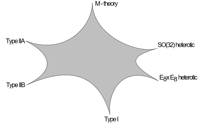
Accordingly, each of the exceptional invariant cocycles on super Minkowski spacetime defines a super p-brane sigma model. These happen to be the fundamental Green-Schwarz superstring and the fundamental supermembrane that appear in, or rather that define string theory and M-theory (“M-theory” is a “non-committal” shorthand for “membrane theory”, (Hořava-Witten 95, p. 2) – a fact known as the “old brane scan” (Achúcarro-Evans-TownsendWiltshire 87).

Now in higher generalization of how an invariant 2-cocycle on some super Minkowski spacetime corresponds to a central super-Lie algebra extension of it to a higher dimensional spacetime, so every higher cocycle, i.e. every $p+2$-cocycle for $p \geq 1$, corresponds to a super Lie (p+1)-algebra extension of super Minkowski spacetime, sometimes called an “extended super Minkowski spacetime”. It turns out that on the super Lie n-algebra extensions defined by the cocycles for the super-string and the super-membrane make further invariant higher cocycles appear. Interpreting these in turn as higher WZW models for super p-branes it turns out that they correspond to the D-branes and to the M5-brane that appear in string theory/M-theory. This generalizes the old brane scan to a tree-like structure of higher invariant extensions that may be called the brane bouquet of string theory/M-theory, since it neatly organizes the complete super p-brane content purely in terms of super Lie n-algebra theory (FSS 13).

Moreover, it turns out that on cocycles of super Lie n-algebras there is a natural higher Lie theoretic operation of double dimensional reduction: the image in rational homotopy theory of the adjunction unit for the “cyclification” adjunction (free loop space homotopy quotiented by loop rotation). Applying this to the brane bouquet turns out to yield relations between the super Lie $n$-algebraic cocycles that embody all the dualities in string theory at the level of rational homotopy theory: the KK-compactification from M-theory to type IIA string theory, the T-duality of the latter to type IIB string theory, the S-duality of the latter, and its relation to F-theory (FSS 16a, FSS 16b).

Notice that all this concerns fundamental super p-branes (sometimes referred to as “probe $p$-branes”) – in generalization of “fundamental particles” and “fundamental string” – and in contrast to “solitonic $p$-branes” or “black branes”. In fact the black branes (that appear for notably in the AdS/CFT correspondence) follow from the fundamental super p-branes: their worldvolumes are the BPS state solutions to the supergravity equations of motion which express but the consistent globalization of the fundamental super p-brane sigma models (Bergshoeff-Sezgin-Townsend 87), and moreover their worldvolume theories are but the perturbation theory of the fundamental super p-branes about these asymptotic singular loci (Claus-Kallosh-vanProeyen 97, Claus-Kallosh-Kumar-Townsend 98).

Hence a fair bit of the folklore structure of string theory/M-theory is (re-)discovered by systematic classification of the invariant higher extensions of super Minkowski spacetimes in super Lie n-algebra homotopy theory. But by the discussion at geometry of physics – supersymmetry, the relevant super-Minkowski spacetimes are themselves already classified as the consecutive ordinary invariant extensions of just the superpoint (we review this below). In conclusion then, a fair bit of the structure of string theory/M-theory is (re-)discovered by a systematic classification of the consecutive invariant higher extension of the superpoint in super Lie n-algebra homotopy theory. This is what we discuss here.

Computationally, all the these cocycles in the brane bouquet exist due to special Fierz identities (which we discuss below), namely due to special spinoral higher Clebsch-Gordan coefficients that express the tensor-product operation in the real representation ring of the spin groups in the given dimensions (D’Auria-Fré-Maina-Regge 82, D’Auria-Fré 82a, D’Auria-Fré 82b)).

Hence there is a tight interplay between spinorial representation theory, super-algebraic higher Lie theory, spacetime that gives rise to a finite system of exceptional structures: the super p-branes. This is what we discuss here.

$\,$

$\,$

$\,$

$\,$

$\,$

In order to put our discussion in perspective, we start by surveying some

• History and background.

Then in order to lay the basis of all our discussion to follow, which is super higher Lie theory, we recall super Lie algebras and discuss their generalization to super L-∞ algebras (whose formal duals are called “FDA”s in the physics literature):

• Super L-infinity cohomology and FDAs.

We will be associating a fundamental $p$-brane with each invariant super $L_\infty$-cocycle. We explain how this is given by a variant of the operation of higher Lie integration in

• From L-infinity-cocycles to higher WZW models

The basic example of super Lie algebras that induces all phenomena to follow are the super-translation parts of supersymmetry algebras, the super Minkowski spacetimes introduced in detail in geometry of physics – supersymmetry. Since here we frequently need to refer to these structures, we recall their definition again in

• Super Minkowski spacetimes.

The key phenomena to be discussed are then the non-trivial invariant cocycles in the super-Lie algebra cohomology of super Minkowski spacetimes (sometimes called tau cohomology in the physics literature). Computationally these correspond to certain identities satisfied by qadrilinear expressions in Majorana spinors. Such relations are an example of Fierz identities and so we pause to explain these in

• Fierz identities.

This then gives rise to the “old brane scan” of Green-Schwarz super-string and super-membranes, which is the classification of the $Spin$-invariant super-Lie algebra cohomology of super Minkowski spacetimes (tau cohomology):

• The super-string and the super-membrane.

Using our previously established general theory of super-L-∞ algebra cohomology, we see that the cocycles in the old brane scan classify higher central extensions of super Minkowski spacetimes, namely super Lie n-algebras called extended super Minkowski spacetimes:

• Extended super Minkowski spacetimes

A key point then is that these super Lie n-algebras obtained from super Minkowski spacetime, turn out to carry further super $L_\infty$-cocycles, not present on the plain super Minkowski spacetimes. These correspond to all the D-branes and to the M5-branes. This we discuss in

• The super D-branes and the M5-brane

This gives a tree of consecutive invariant universal higher central extensions of super Lie n-algebras, originating from the superpoint: the brane bouquet. Next we descend these iterated central extensions to single but non-central higher cocycles. The result turns out to be the image in rational homotopy theory of the classifying maps of the background fields in string theory/M-theory: the B-field-twisted RR-fields and the M-flux fields. This we discuss in

• Fields.

There turn out to be special relations among these. In particular passing from super-L-∞ algebra cohomology to the corresponding cyclic cohomology turns out to be the formal dual operation of what in physics is called double dimensional reduction of branes (here: of their background fields). This crucial operation we discuss in

• Double dimensional reduction .

By systematically applying this super Lie n-algebraic formalization of double dimensional reduction via cyclic cohomology, we discover all the pertinent dualities in string theory, rationally:

• Dualities.

History and background

Below we present fundamental super p-branes as exceptional algebro-geometric structures that are discovered by applying the magnifying glass (namely a Whitehead tower construction) of super Lie n-algebra homotopy theory to the atom of superspace: the superpoint, following (FSS 13, FSS 15, FSS 16a, FSS 16b).

This is not the perspective from which super p-branes were arrived at historically. In order to put our discussion into perspective, here we briefly review some of the historical background.

$\,$

Perturbativestring theory on geometric backgrounds is defined by the Neveu-Schwarz-Ramond model, namely by sigma-model 2d super conformal field theories (of central charge 15) on worldsheets $\Sigma$ that are super Riemann surfaces, with target spaces $X$ that are ordinary (i.e. “bosonic”) spacetime manifolds.

These worldsheet field theories are induced from action functionals, namely from variants of the standard energy functional (Polyakov action) on the mapping space $[\Sigma,X]$ of smooth functions

$$\phi \;\colon\; \Sigma \longrightarrow X$$

from the worldsheet $\Sigma$ to target spacetime $X$.

The central theorem of perturbative superstring theory (the no ghost theorem with GSO projection) says that the excitation spectrum of such a 2d SCFT are the quanta of the perturbations of a higher dimensional effective supergravity field theory on target spacetime, hence transforms under supersymmetry on target spacetime.

This is the fundamental prediction of the assumption of fundamental strings:

1. assuming that the fundamental particles that run in Feynman diagrams are fundamentally (at high energy) the ground state modes of a fundamental string,

2. demanding that there are fermionic particles among these,

implies

1. that the string must be the spinning string (have fermions in its worldsheet theory), which in turn implies…

2. that it is the superstring (worldsheet supersymmetry mixes the worldsheet bosons and fermions), precisely: the Neveu-Schwarz-Ramond superstring, which then in addition implies…

3. that its target space effective field theory is a supergravity theory, hence that also the effective target space fields exhibit local supersymmetry (i.e. “high energy supersymmetry”, different from “low energy supersymmetry” that the LHC was looking for).

main theorem of perturbative super-string theory
$\underset{\text{spinning string}}{\underbrace{\text{fermions} \;+\; \text{strings}}} \;=\; \text{superstring} \;\Rightarrow\; \text{supergravity}$

The first step in this implication (identifying the spinning string as the superstring) is fairly straightforward (in fact this is how the concept of supersymmetry was discovered in “the west”, in the first place), but the second step (that the superstring excitations necessarily are quanta of a spacetime supergravity theory) appears as a miracle from the point of view of the Neveu-Schwarz-Ramond superstring. It comes out this way by non-trivial computation, but is not manifest in the theory.

In order to improve on this situation, Michael Green and John Schwarz searched for and found (Green-Schwarz 81, Green-Schwarz 82 Green-Schwarz 84, for the history see Schwarz 16, slides 24-25) a suitably equivalent string action functional that would manifestly exhibit spacetime supersymmetry. Acordingly, this is now called the Green-Schwarz action functional.

action functional for superstring	manifest supersymmetry
Neveu-Ramond-Schwarz super-string	on worldsheet
Green-Schwarz super-string	on target spacetime

The basic idea is to pass to the evident supergeometric analogue of the bosonic string action:

Let $\Sigma$ be a closed manifold of dimension 2 – representing the abstract worldsheet of a string. Let $(X,g)$ be a pseudo-Riemannian manifold – representing a purely gravitational spacetime background. Then the action functional governing the bosonic string propagating in this spacetime is the functional

$$\exp(\tfrac{i}{\hbar} S_{bos}) \;\colon\; [\Sigma,X] \longrightarrow \mathbb{R}/_{\hbar}\mathbb{Z}$$

on the smooth mapping space $[\Sigma,X]$ (of smooth functions $\Sigma \to X$), that simply assigns the proper relativistic volume of the image of the worldsheet $\Sigma$ in spacetime:

$$(\Sigma\overset{\phi}{\longrightarrow} X) \;\mapsto\; S_{kin}(\phi) \coloneqq \int_\Sigma vol_{\phi^\ast g} \,.$$

(This is the Nambu-Goto action. It is classically equivalently to the Polyakov action which is the genuine starting point for the quantum Neveu-Ramond-Schwarz super-string. Howver, since, as we discuss below, the Green-Schwarz action naturally generalizes to that of other p-branes it is more natural to consider the Nambu-Goto form of the action here.)

When here $(X,g)$ is generalized to a superspacetime supermanifold with orthogonal structure encoded by a super-vielbein $e$, then the same form of the action functional still makes sense and produces a functional on the supergeometric mapping space $[\Sigma,X]$. Moreover, by construction this action functional now is invariant under the superisometry group of $(X,g)$, hence under global spacetime supersymmetry.

$$\array{ \text{symmetry of worldsheet theory} \\ \array{ && \Sigma \\ & {}^{\mathllap{\phi}}\swarrow && \searrow^{\mathrlap{\phi'}} \\ X &&\underset{\simeq}{\longrightarrow}&& X } \\ \text{super-isometry of target spacetime} }$$

However, Green and Schwarz noticed that this kinetic action functional $\phi \mapsto \int_\Sigma vol_{\phi^\ast e}$ does not quite yield dynamics that is equivalent to that of the Neveu-Schwarz-Ramond super-string: when the equations of motion hold (“on shell”) it has more fermionic degrees of freedom than present in the Neveu-Ramond-Schwarz super-string. The key insight of Green and Schwarz was that one may add an extra summand $S_{WZW}$ (whose notation we explain in a moment) to the plain super-Nambu-Goto action $S_{kin}$, such that the resulting action functional enjoys a further 1-parameter symmetry, called kappa-symmetry. This is the Green-Schwarz action functional:

$$S_{GS} = S_{kin} + S_{WZW} \,.$$

Moreover, they showed that restricting the dynamics of the Green-Schwarz superstring to the $\kappa$-symmetric states, then it does become equivalent, classically to that of the Neveu-Ramond-Schwarz super-string.

Finally they showed that when gauge fixing the Green-Schwarz action functional to light-cone gauge (which is possible whenever target spacetime admits two lightlike Killing vector) then the Green-Schwarz string may be quantized by a standard procedure and the resulting quantum dynamics is equivalent to that of the Neveu-Schwarz-Ramond super-string. This provides the desired conceptual proof for the observed local target spacetime supersymmetry of super-string effective field theory, at least for backgrounds that admit two lightlike Killing vectors. (The quantization of the Green-Schwarz superstring away from light cone gauge remains an open problem.)

While Green-Schwarz’s extra kappa-symmetry term $S_{WZW}$ this serves a clear purpose as a means to an end, originally its geometric meaning was mysterious. However, in (Henneaux-Mezincescu 85) it was observed (expanded on in (Rabin 87, Azcarraga-Townsend 89, Azcarraga-Izquierdo 95,chapter 8)), that the Green-Schwarz action functional describing the super-string in $d+1$-dimensions does have a neat geometrical interpretation: it is simply the (parameterized) Wess-Zumino-Witten model for

1. target space being locally super Minkowski spacetime $\mathbb{R}^{d-1,1|\mathbf{N}}$ regarded as the coset supergroup

   $$\mathbb{R}^{d-1,1\vert \mathbf{N}} \;\simeq\; Iso(\mathbb{R}^{d-1,1\vert \mathbf{N}}) / Spin(d-1,1)$$

   for $\mathbf{N}$ a real spin representation (the “number of supersymmetries”), $Iso(\mathbb{R}^{d-1,1\vert \mathbf{N}})$ the corresponding super Poincaré group and $Spin(d-1,1)$ its Lorentz-signature Spin subgroup;

2. WZW-term being a local potential for the unique (up to rescaling, if it exists) $Spin(d-1,1)$-invariant super Lie algebra 3-cocycle $\mu_{F1}$ on the super Poincaré Lie algebra $\mathfrak{iso}(\mathbb{R}^{d-1,1\vert \mathbf{N}})$, with components locally given by the Gamma-matrices of the given Clifford algebra representation; in terms of the super vielbein $(e^a, \psi^\alpha)$:

   $$\mu_{F1} = \overline{\psi} \wedge \Gamma_A \psi \wedge e_a$$

   and so in components the bi-fermionic component of $\mu_{F1}$ is

   $$(\mu_{F1})_{a \alpha \beta} = \Gamma_{a \alpha \beta}$$

   and all other components vanish.

More in detail, just as ordinary Minkowski spacetime $\mathbb{R}^{d-1,1}$ may be identified with the translation group along itself, with canonical linear basis of left invariant 1-forms given by the canonical vielbein field

$$\{e^a \coloneqq \mathbf{d}x^a\}_{a = 0}^{d-1} \,,$$

where $\{x^a\}$ are the canonical coordinates on $\mathbb{R}^{d-1,1}$, so super Minkowski spacetime $\mathbb{R}^{d-1,1\vert \mathbf{N}}$ for some real spin representation $\mathbf{N}$ is characterized as the supergroup whose left invariant 1-forms constitute the $\mathbb{Z} \times \mathbb{Z}/2\mathbb{Z}$-bigraded differential with generators the super-vielbein

$$\underset{deg = (1,even)}{\underbrace{e^a}} \;\coloneqq\; \mathbf{d}x^a + \overline{\theta}\Gamma^a \mathbf{d} \theta \;\;\;\,,\;\;\;\;\;\;\;\;\;\; \underset{deg = (1,odd)}{\underbrace{\psi^\alpha}} \;\coloneqq\; \mathbf{d}\theta^\alpha \,,$$

where $(x^a, \theta^\alpha)$ are the canonical coordinates on $\mathbb{R}^{d-1,1\vert \mathbf{N}}$, with the odd-graded elements $\{\theta^\alpha\}$ spanning the given real Spin(d-1,1)-representation $\mathbf{N}$ with Clifford algebra generators $\{\Gamma^a\}$.

Now while ordinary Minkowski spacetime $\mathbb{R}^{d-1,1}$ is an abelian group, reflected by the fact that its left-invariant 1-forms are all closed

$$\mathbf{d}e^a = 0 \;\;\;\;\;\; on \; \mathbb{R}^{d-1,1} \,,$$

the key phenomenon of supersymmetry (that two fermions pair to a bosons) means that $\mathbb{R}^{d-1,1\vert \mathbf{N}}$ is slightly non-abelian, reflected by the fact that the super-vielbein is not closed

$$\mathbf{d} e^a = \overline{\psi} \wedge \Gamma^a \psi \;\,,\;\;\;\;\;\; \mathbf{d} \psi^\alpha = 0 \,.$$

This elementary effect is the source of all the rich structure seen in the Green-Schwarz super-string and generally in all super p-brane theory. (The above differential is equivalently that in the Chevalley-Eilenberg algebra of super Minkowski spacetime, hence its cohomology is the super-Lie algebra cohomology of super Minkowski spacetime. In parts of the physics literature this is referred to a “tau cohomology”.)

In particular, for special combinations of spacetime dimension $d$ and number of supersymmetries $\mathbf{N}$ (i.e. real spin representation $N$) then the 3-form

$$\mu_{F1} = \overline{\psi} \wedge \Gamma_a \psi \wedge e^a$$

is a non-trivial super Lie algebra cocycle on $\mathbb{R}^{d-1,1\vert \mathbf{N}}$, in that $\mathbf{d}\mu_{F1} = 0$ and so that there is no left invariant differential form $b$ with $\mathbf{d}b = \mu_{F1}$ (beware here the left-invariance condition: there are of course non-left-invariant potentials for $\mu_{F1}$, and in fact these are exactly the possible Lagrangian densities for the WZW action functional $S_{WZW}$).

This happens notably for

1. $d = 10$ and $\mathbf{N} = (1,0) = \mathbf{16}$ (heterotic string)

2. $d = 10$ and $\mathbf{N} = (2,0) = \mathbf{16} + \mathbf{16}$ (type IIB superstring)

3. $d = 10$ and $\mathbf{N} = (1,1) = \mathbf{16} + \mathbf{16}^\ast$ (type IIA superstring).

(It also happens in some lower dimensions, where however the corresponding Neveu-Schwarz-Ramond string develops a conformal anomaly after [8quantization]] (“non-critical strings”). This classification of cocycles is part of what has come to be known as the brane scan in superstring theory, see below.)

In this equivalent formulation, the Green-Schwarz action functional for the superstring has the following simple form:

Let $(X,e)$ be a superspacetime, hence a supermanifold $X$ equipped with a super-vielbein $e$ (super-orthogonal structure) which is locally modeled on $\mathbb{R}^{d-1,1\vert \mathbf{N}}$ (technically: a torsion-free super-Cartan geometry modeled on $Spin(d-1,1) \hookrightarrow Iso(\mathbb{R}^{d-1,1\vert \mathbf{N}})$). Write $\mu_{F1}^X \in \Omega^3(X)$ for the super differential form on $X$ which is the induced definite globalization of the cocycle $\mu_{F1}$ over $X$. For $U \subset X$ any contractible subspace, then the restriction of $\mu^X_{F1}|_{U} \in \Omega^3(U)$ of $\mu_{F1}^X$ to $U$ is exact, and hence admits a potential $B_U \in \Omega^2(U)$, i.e. such that $\mathbf{d} B = \mu^X_{F1}|_U$.

Then for $\Sigma$ a 2-dimensional closed manifold, the Green-Schwarz action functional

$$\exp(\tfrac{i}{\hbar} S_{GS}) \;\colon\; [\Sigma,X]_U \longrightarrow \mathbb{R}/_{\hbar} \mathbb{Z}$$

is the function on the super-smooth mapping space $[\Sigma,X]_U$ of morphisms of supermanifolds $\phi \colon \Sigma \to X$ which factor through $U$, given by

$$\phi \;\mapsto\; \int_\Sigma vol_{\phi^\ast e} \;+\; \int_\Sigma \phi^\ast B_U \;\;\;\,,\;\;\;\;\;\;\;\;\; \mathbf{d} B_U = \mu^X_3|_U \,.$$

In order to get rid of the restriction to some chart $U \subset X$ one needs to add global data. The need for this is at least mentioned briefly in (Witten 86, p. 261 (17 of 20)), but seems to have otherwise been ignored in the physics literature. The general solution is to promote the local potentials $B$ to the connection $\hat B$ on a super gerbe (FSS 13). This is a choice of higher prequantization

$$\array{ && \mathbf{B}^{2}(\mathbb{R}/_\hbar \mathbb{Z}) & \text{prequantization} \\ & {}^{\mathllap{\hat B}}\nearrow & \downarrow^{\mathrlap{curv}} \\ X &\underset{\mu^X_{F1}}{\longrightarrow}& \mathbf{\Omega}^3 & \text{3-form curvature} } \,.$$

Writing $\int_\Sigma \phi^\ast \hat B$ for the volume holonomy of a circle 2-bundle with connection $\hat B$, then the globally defined Green-Schwarz sigma model

$$\exp(\tfrac{i}{\hbar} S_{GS}) \;\colon\; [\Sigma, X] \longrightarrow \mathbb{R}/_\hbar\mathbb{Z}$$

is given by

$$\phi \;\mapsto\; \int_\Sigma vol_{\phi^\ast} + \int_\Sigma \phi^\ast \hat B \;\;\,, \;\;\;\;\;\;\; curv(\hat B) = \mu_{F1}^X \,.$$

This form of the Green-Schwarz action functional for the string has evident generalization to other p-branes. Whenever there is a Spin(d-1,1)-invariant $(p+2)$-cocycle $\mu_{p+2}$ on $\mathbb{R}^{d-1,1\vert \mathbf{N}}$, then one may ask for a higher gerbe (higher prequantum line bundle) $\hat C$ with curvature $\mu^X_{p+2}$ and consider the analogous functional.

The triples $(d,\mathbf{N},p)$ (spacetime dimension, number of supersymmetries, dimension of brane) such that

$$\mu_{p+2} \;\coloneqq\; \overline{\psi} \wedge \Gamma^{a_1 \cdots a_p} \psi \wedge e_{a_1} \wedge \cdots \wedge e_{a_p}$$

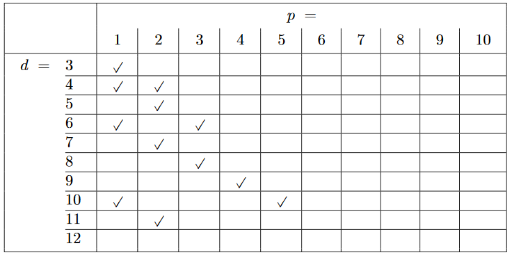
is a nontrivial cocycle, hence for which there is such a Green-Schwarz action functional for $p$-branes on $\mathbb{R}^{d-1,1\vert \mathbf{N}}$ may be classified and form what is called the brane scan (Achúcarro-Evans-TownsendWiltshire 87, Brandt 12-13):

The graphics on the left is from (Duff 87). The diagonal lines indicate double dimensional reduction, taking a $(p+1)$-brane in $(d+1)$ dimensions to a $p$-brane in $d$-dimensions.

For instance for $(d = 11, \; \mathbf{N} = \mathbf{32}, \; p = 2)$ one finds a cocycle, and the corresponding GS-action functional is that of the fundamental M2-brane.

This was a striking confluence of brane physics and classification of super Lie algebra cohomology. But just as striking as the matching, was what it lacked to match: the D-branes and the M5-brane ($d = 11$, $p = 5$) are lacking from the old brane scan. Incidentally, these lacking branes are precisely those branes on which the branes that do appear on the brane scan may end, equivalently those branes that have higher gauge fields on their worldvolume (tensor multiplets).

An action functional for the M5-brane analogous to a Green-Schwarz action functional was found in (BLNPST 97, APPS 97). It is again the sum of a kinetic term and a WZW-like term, but the WZW-like term does not come from a cocycle on a (super-)group.

In order to deal with this, it was suggested in (CAIB 99, Sakaguchi 00, Azcarraga-Izquierdo 01) that there is an algebraic structure called “extended super-Minkowski spacetimes” that generalizes super Minkowski spacetime and serves to unify the Green-Schwarz-like models for the D-branes and the M5-brane with the original Green-Schwarz models for the string and the M2-brane.

These extended super-Minkowski spacetimes carry algebraic analogs of super Lie algebra cocycles, such that the relevant terms for the D-branes and the M5-brane do appear after all, hence such that all the branes in string theory/M-theory are unified. In fact these “extended super-Minkowski spacetimes” are precisely the “FDA”s that have been introduced before in the D'Auria-Fré formulation of supergravity and what became identified as the 7-cocycle for the M5-brane this way had earlier been recognized algebraically as an stepping stone for an elegant re-derivation of 11-dimensional supergravity (D’Auria-Fré 82).

The (higher) geometric meaning of these constructions was found in (Fiorenza-Sati-Schreiber 13): these algebraic structures of “extended super-Minkowski spacetimes”/FDAs are precisely the Chevalley-Eilenberg algebras of super Lie n-algebra-extensions of super-Minkowski spacetime which are classified by the cocycles that serve as the GS-WZW terms of the $p_1$-branes that may end on those $p_2$-branes whose cocycles are carried by the extended super-Minkowski spacetime.

Hence the missing $p$-branes in the old brane scan (classifying just cocycles on super Lie algebras) do appear as one generalizes (super) Lie algebras to (super) strong homotopy Lie algebras = L-infinity algebras. Moreover, each brane intersection law (one brane species may end on another) is now matched to a super $L_\infty$-algebra extension and so the old brane scan is generalized to a tree of branes The brane bouquet:

Each item in this bouquet denotes a super L-infinity algebra and each arrow denotes an L-infinity extension classified by a cocycle which encodes the GS-WZW term of the brane named by the domain of the arrow. Moreover, arrows pass exactly from one brane species to the brane species that may end on the former.

In (Fiorenza-Sati-Schreiber 13) it is shown that all these super L-infinity algebras Lie integrate to smooth super-n-groups, and all the cocycles Lie integrate to super-gerbes on these, such that the induced volume holonomy is the relevant generalized GS-WZW term. For detailed exposition see at Structure Theory for Higher WZW Terms.

With this generalized perspective, now the Green-Schwarz-type action functionals describe all the p-branes in string theory/M-theory.

Again, in order to make this generally true one needs to apply a higher prequantization – a choice of line (p+1)-bundle with connection – in order to globalize the WZW-terms (Fiorenza-Sati-Schreiber 13)

$$\array{ && \mathbf{B}^{p+1}(\mathbb{R}/_\hbar \mathbb{Z}) & \text{prequantization} \\ & {}^{\mathllap{\hat A_{p+1}}}\nearrow & \downarrow^{\mathrlap{curv}} \\ X &\underset{\mu^X_{p+2}}{\longrightarrow}& \mathbf{\Omega}^{p+2} & (p+2)\text{-form curvature} } \,.$$

Hence $\hat A_{p+1}$ is the actual background field that the $p$-brane couples to. There is considerably more information in $\hat A_p$ than in its curvature $curv(\hat A_{p+1}) = \mu_{p+2}$. For instance for the M2-brane one may find the local super moduli space for local choices of $\hat A_{p+1}$ for the given $\mu_{4}$ on KK-compactifications to $d = 4$. It turns out that the bosonic body of this moduli space is the exceptional tangent bundle on which the U-duality group E7 has a canonical action (see at From higher to exceptional geometry).

This highlights that Green-Schwarz functionals capture fundamental (“microscopic”) aspects of $p$-branes. In contrast, often $p$-branes are discussed in their solitonic incarnation as black branes. These solitonic branes sit at asymptotic boundaries of anti-de Sitter spacetime and carry conformal field theories, related to the ambient supergravity by AdS-CFT duality.

This phenomenon is indeed a consequence of the fundamental Green-Schwarz branes:

Consider a 1/2-BPS state solution of type II supergravity or 11-dimensional supergravity, respectively. These solutions locally happen to have the same classification as the Green-Schwarz branes. Hence we may consider a configuration $\phi \colon \Sigma \to X$ of the corresponding fundamental $p$-brane which embeds $\Sigma$ into the asymptotic AdS boundary of the given 1/2 BPS spacetime $X$. Then it turns out that restricting the Green-Schwarz action functional to small fluctuations around this configuration, and applying a diffeomorphism gauge fixing, then the resulting action functional is that of a supersymmetric conformal field theory on $\Sigma$ as in the AdS-CFT dictionary:

fundamental $p$-brane	-fluctuations about asymptotic AdS configuration$\to$	solitonic $p$-brane
Green-Schwarz action functional		super-conformal field theory

(Claus-Kallosh-Proeyen 97, Claus-Kallosh-Kumar-Townsend 98, AFFFTT 98 Pasti-Sorokin-Tonin 99)

In fact the BPS-state condition itself is neatly encoded in the Green-Schwarz action functionals: by construction they are invariant under the spacetime superisometry group. Hence the Noether theorem implies that there are corresponding conserved currents, whose Dickey bracket forms a super-Lie algebra extension of the Lie algebra of supersymmetries.

$$\array{ \left\{ \array{ X && \overset{=}{\longrightarrow} && X \\ & {}_{\mathllap{\hat C}}\searrow &\swArrow& \swarrow_{\mathrlap{\hat C}} \\ && \mathbf{B}^{p+1}(\mathbb{R}/_{\hbar} \mathbb{Z}) } \right\} &\longrightarrow& \left\{ \array{ X && \overset{\simeq}{\longrightarrow} && X \\ & {}_{\mathllap{\hat C}}\searrow &\swArrow& \swarrow_{\mathrlap{\hat C}} \\ && \mathbf{B}^{p+1}(\mathbb{R}/_{\hbar} \mathbb{Z}) } \right\} &\longrightarrow& \left\{ \array{ X && \overset{\simeq}{\longrightarrow} && X } \right\} \\ \text{topological currents} && \text{Noether currents} && \text{symmetries} }$$

Here the “$\swArrow$” filling the triangles is the non-trivial gauge transformation by which the WZW term (as any WZW term) is preserved under the symmetries (instead of being fixed identically). It is the information in this transformations which makes the currents form an extension of the symmetries.

Here this yields the famous brane charge extensions of the super-isometry super Lie algebra of the schematic form

$$\{Q_\alpha, Q_\beta\} \;=\; (C \Gamma^a_{\alpha \beta}) P_a \;+\; (C \Gamma^{a_1 \cdots a_p})_{\alpha \beta} Z_{a_1, \cdots, a_p}$$

(for $Q$ a Killing spinor and $P$ its corresponding Killing vector) known as the type II supersymmetry algebra and the M-theory supersymmetry algebra, respectively (Azcárraga-Gauntlett-Izquierdo-Townsend 89). In fact it yields super-Lie n-algebra extensions of which the familiar super Lie algebra extensions are the 0-truncation (Sati-Schreiber 15, Khavkine-Schreiber 16).

In summary, the nature and classification of Green-Schwarz action functionals captures in a mathematically precise way a good deal of the core structure of string/M-theory.

In fact, the super Lie-n algebraic perspective on the Green-Schwarz functionals via the brane bouquet also solves the following open problem on M-branes:

it is famously known from Freed-Witten anomaly-cancellation that the D-brane charges are not in fact just in de Rham cohomology in every second degree, but are in twisted K-theory, hence rationally in twisted de Rham cohomology, with the twist being the F1-brane charge (from the fundamental). It is an open problem to determine what becomes of these twisted K-theory charge groups as one lifts F1/D$p$-branes in string theory to M2/M5-branes in M-theory.

	intersecting branes	charges in generalized cohomology theory
string theory	F1/Dp-branes	twisted K-theory
M-theory	M2/M5-branes	???

Notice that there are “microscopic degrees of freedom” of the theory encoded by the choice of generalized cohomology theory here, generalizing the extra degrees of freedom in the choice of a WZW-term already mentioned above. In general for $E$ a cohomology theory and $E \longrightarrow E \otimes \mathbb{Q}$ its Chern character map (for instance from topological K-theory to ordinary cohomology in every second degree), then a choice of genuine charges is the extra information encoded in a lift

$$\array{ && E \\ & {}^{\mathllap{\text{true charge}}}\nearrow & \downarrow^{\mathrlap{ch}} \\ X &\underset{\text{rational} \atop \text{charge}}{\longrightarrow}& E \otimes \mathbb{Q} }$$

But rationally The brane bouquet allows to derive this from first principles:

Above we saw that the naive cocycles of the D-branes and of the M5-brane are not defined on the actual spacetime, but on some “extended” spacetime, which is really a smooth super infinity-groupoid extension of spacetime. Hence we should ask if these cocycles descend to the actual super-spacetime while picking up some twists.

One may prove that:

• the F1/D$p$-brane GS-WZW cocycles descend to 10d type II superspacetime to form a single cocycle in rational twisted K-theory, just as the traditional lore reqires (Fiorenza-Sati-Schreiber 16);

• the M2/M5 GS-WZW cocycles descent to 11d superspacetime to form a single cocycle with values in the rational 4-sphere (Fiorenza-Sati-Schreiber 16).

This has implications on some open conjectures regarding M-theory, for more on this see Equivariant cohomology of M2/M5-branes.

$\,$

We now explain all this in detail.

$\,$

Super $L_\infty$-cohomology and FDAs

We recall super Lie algebras, and amplify their formal dual description in terms of their Chevalley-Eilenberg algebras. This makes it immediate to see what super L-∞ algebras are, again they are conveniently expressed (if they are of finite type) via their formal dual Chevalley-Eilenberg algebras.

Definition

A super Lie algebra is a Lie algebra internal to the symmetric monoidal category $sVect = (Vect^{\mathbb{Z}/2}, \otimes_k, \tau^{super} )$ of super vector spaces. Hence this is

1. a super vector space $\mathfrak{g}$;

2. a homomorphism

   $$[-,-] \;\colon\; \mathfrak{g} \otimes_k \mathfrak{g} \longrightarrow \mathfrak{g}$$

   of super vector spaces (the super Lie bracket)

such that

1. the bracket is skew-symmetric in that the following diagram commutes

   $$\array{ \mathfrak{g} \otimes_k \mathfrak{g} & \overset{\tau^{super}_{\mathfrak{g},\mathfrak{g}}}{\longrightarrow} & \mathfrak{g} \otimes_k \mathfrak{g} \\ {}^{\mathllap{[-,-]}}\downarrow && \downarrow^{\mathrlap{[-,-]}} \\ \mathfrak{g} &\underset{-1}{\longrightarrow}& \mathfrak{g} }$$

   (here $\tau^{super}$ is the braiding natural isomorphism in the category of super vector spaces)

2. the Jacobi identity holds in that the following diagram commutes

   $$\array{ \mathfrak{g} \otimes_k \mathfrak{g} \otimes_k \mathfrak{g} && \overset{\tau^{super}_{\mathfrak{g}, \mathfrak{g}} \otimes_k id }{\longrightarrow} && \mathfrak{g} \otimes_k \mathfrak{g} \otimes_k \mathfrak{g} \\ & {}_{\mathllap{[-,[-,-]]} - [[-,-],-] }\searrow && \swarrow_{\mathrlap{[-,[-,-]]}} \\ && \mathfrak{g} } \,.$$

Externally this means the following:

Proposition

A super Lie algebra according to def. is equivalently

1. a $\mathbb{Z}/2$-graded vector space $\mathfrak{g}_{even} \oplus \mathfrak{g}_{odd}$;

2. equipped with a bilinear map (the super Lie bracket)

   $$[-,-] : \mathfrak{g}\otimes_k \mathfrak{g} \to \mathfrak{g}$$

   which is graded skew-symmetric: for $x,y \in \mathfrak{g}$ two elements of homogeneous degree $\sigma_x$, $\sigma_y$, respectively, then

   $$[x,y] = -(-1)^{\sigma_x \sigma_y} [y,x] \,,$$

3. that satisfies the $\mathbb{Z}/2$-graded Jacobi identity in that for any three elements $x,y,z \in \mathfrak{g}$ of homogeneous super-degree $\sigma_x,\sigma_y,\sigma_z\in \mathbb{Z}_2$ then

   $$[x, [y, z]] = [[x,y],z] + (-1)^{\sigma_x \cdot \sigma_y} [y, [x,z]] \,.$$

A homomorphism of super Lie algebras is a homomorphisms of the underlying super vector spaces which preserves the Lie bracket. We write

$$sLieAlg$$

for the resulting category of super Lie algebras.

Definition

For $\mathfrak{g}$ a super Lie algebra of finite dimension, then its Chevalley-Eilenberg algebra $CE(\mathfrak{g})$ is the super-Grassmann algebra on the dual super vector space

$$\wedge^\bullet \mathfrak{g}^\ast$$

equipped with a differential $d_{\mathfrak{g}}$ that on generators is the linear dual of the super Lie bracket

$$d_{\mathfrak{g}} \;\coloneqq\; [-,-]^\ast \;\colon\; \mathfrak{g}^\ast \to \mathfrak{g}^\ast \wedge \mathfrak{g}^\ast$$

and which is extended to $\wedge^\bullet \mathfrak{g}^\ast$ by the graded Leibniz rule (i.e. as a graded derivation).

$\,$

Here all elements are $(\mathbb{Z} \times \mathbb{Z}/2)$-bigraded, the first being the cohomological grading $n$ in $\wedge^\n \mathfrak{g}^\ast$, the second being the super-grading $\sigma$ (even/odd).

For $\alpha_i \in CE(\mathfrak{g})$ two elements of homogeneous bi-degree $(n_i, \sigma_i)$, respectively, the sign rule is

$$\alpha_1 \wedge \alpha_2 = (-1)^{n_1 n_2} (-1)^{\sigma_1 \sigma_2}\; \alpha_2 \wedge \alpha_1 \,.$$

(See at signs in supergeometry for discussion of this sign rule and of an alternative sign rule that is also in use. )

We may think of $CE(\mathfrak{g})$ equivalently as the dg-algebra of left-invariant super differential forms on the corresponding simply connected super Lie group .

The concept of Chevalley-Eilenberg algebras is traditionally introduced as a means to define Lie algebra cohomology:

Definition

Given a super Lie algebra $\mathfrak{g}$, then

1. an $n$-cocycle on $\mathfrak{g}$ (with coefficients in $\mathbb{R}$) is an element of degree $(n,even)$ in its Chevalley-Eilenberg algebra $CE(\mathfrak{g})$ (def. ) which is $d_{\mathbb{g}}$ closed.

2. the cocycle is non-trivial if it is not $d_{\mathfrak{g}}$-exact

3. hene the super-Lie algebra cohomology of $\mathfrak{g}$ (with coefficients in $\mathbb{R}$) is the cochain cohomology of its Chevalley-Eilenberg algebra

   $$H^\bullet(\mathfrak{g}, \mathbb{R}) = H^\bullet(CE(\mathfrak{g})) \,.$$

The following says that the Chevalley-Eilenberg algebra is an equivalent incarnation of the super Lie algebra:

Proposition

The functor

$$CE \;\colon\; sLieAlg^{fin} \hookrightarrow dgAlg^{op}$$

that sends a finite dimensional super Lie algebra $\mathfrak{g}$ to its Chevalley-Eilenberg algebra $CE(\mathfrak{g})$ (def. ) is a fully faithful functor which hence exibits super Lie algebras as a full subcategory of the opposite category of differential-graded algebras.

This makes it immediate how to generalize to super L-infinity algebras:

Definition

A super L-∞ algebra is an L-∞ algebra internal to the symmetric monoidal category of super vector spaces (def.).

Explicitly this means the following:

Definition

(super graded signature of a permutation)

Let $V$ be a $\mathbb{Z}$-graded super vector space, hence a $\mathbb{Z} \times (\mathbb{Z}/2)$-bigraded vector space.

For $n \in \mathbb{N}$ let

$$\mathbf{v} = (v_1, v_2, \cdots, v_n)$$

be an n-tuple of elements of $V$ of homogeneous degree $(n_i, s_i) \in \mathbb{Z} \times \mathbb{Z}/2$, i.e. such that $v_i \in V_{(n_i,s_i)}$.

For $\sigma$ a permutation of $n$ elements, write $(-1)^{\vert \sigma \vert}$ for the signature of the permutation, which is by definition equal to $(-1)^k$ if $\sigma$ is the composite of $k \in \mathbb{N}$ permutations that each exchange precisely one pair of neighboring elements.

We say that the super $\mathbf{v}$-graded signature of $\sigma$

$$\chi(\sigma, v_1, \cdots, v_n) \;\in\; \{-1,+1\}$$

is the product of the signature of the permutation $(-1)^{\vert \sigma \vert}$ with a factor of

$$(-1)^{n_i n_j}(-1)^{s_i s_j}$$

for each interchange of neighbours $(\cdots v_i,v_j, \cdots )$ to $(\cdots v_j,v_i, \cdots )$ involved in the decomposition of the permuation as a sequence of swapping neighbour pairs (see at signs in supergeometry for discussion of this combination of super-grading and homological grading).

Now def. is equivalent to the following def. . This is just the definiton for L-infinity algebras, with the pertinent sign $\chi$ now given by def. .

Definition

An super L-∞ algebra is

1. a $\mathbb{Z} \times (\mathbb{Z}/2)$-graded vector space $\mathfrak{g}$;

2. for each $n \in \mathbb{N}$ a multilinear map, called the $n$-ary bracket, of the form

   $$l_n(\cdots) \;\coloneqq\; [-,-, \cdots, -]_n \;\colon\; \underset{n \; \text{copies}}{\underbrace{\mathfrak{g} \otimes \cdots \otimes \mathfrak{g}}} \longrightarrow \mathfrak{g}$$

   and of degree $n-2$

such that the following conditions hold:

1. (super graded skew symmetry) each $l_n$ is graded antisymmetric, in that for every permutation $\sigma$ of $n$ elements and for every n-tuple $(v_1, \cdots, v_n)$ of homogeneously graded elements $v_i \in \mathfrak{g}_{\vert v_i \vert}$ then

   $$l_n(v_{\sigma(1)}, v_{\sigma(2)},\cdots ,v_{\sigma(n)}) = \chi(\sigma,v_1,\cdots, v_n) \cdot l_n(v_1, v_2, \cdots v_n)$$

   where $\chi(\sigma,v_1,\cdots, v_n)$ is the super $(v_1,\cdots,v_n)$-graded signature of the permuation $\sigma$, according to def. ;

2. (strong homotopy Jacobi identity) for all $n \in \mathbb{N}$, and for all (n+1)-tuples $(v_1, \cdots, v_{n+1})$ of homogeneously graded elements $v_i \in \mathfrak{g}_{\vert v_i \vert}$ the followig equation holds

   (1)$$\sum_{{i,j \in \mathbb{N}} \atop {i+j = n+1}} \sum_{\sigma \in UnShuff(i,j)} \chi(\sigma,v_1, \cdots, v_{n}) (-1)^{i(j-1)} l_{j} \left( l_i \left( v_{\sigma(1)}, \cdots, v_{\sigma(i)} \right), v_{\sigma(i+1)} , \cdots , v_{\sigma(n)} \right) = 0 \,,$$

   where the inner sum runs over all $(i,j)$-unshuffles $\sigma$ and where $\chi$ is the super graded signature sign from def. .

A strict homomorphism of super $L_\infty$-algebras

$$is \mathfrak{g}_1 \longrightarrow \mathfrak{g}_2$$

is a linear map that preserves the bidegree and all the brackets, in an evident sens.

A strong homotopy homomorphism (“sh map”) of super $L_\infty$-algebras is something weaker than that, best defined in formal duals, below in def. .

Remark

Special cases of the general concept of super L-∞ algebras def. go by special names:

Let $\mathfrak{g}$ be a super L-∞ algebra.

If $\mathfrak{g}$ is concentrated in even $\mathbb{Z}/2$-degree, it is called an L-∞ algebra.

If the only possibly non-vanishing brackets of $\mathfrak{g}$ are the unary one $[-]$ (which induces the structure of a chain complex on $\mathfrak{g}$) and the binary one, then $\mathfrak{g}$ is equivalently a (super-)dg-Lie algebra.

If $\mathfrak{g}$ is concentrated in $\mathbb{Z}$-degrees 0 to $n-1$ then it is called a super Lie n-algebra.

In particular if $\mathfrak{g}$ is concentrated in degree 0, then it is equivalently a super Lie algebra.

Combining this, if $\mathfrak{g}$ is concentrated in even $\mathbb{Z}/2$-degree and in $\mathbb{Z}$-degree 0 through $n-1$, then it is called a Lie n-algebra.

In particular if $\mathfrak{g}$ is concentrated in $\mathbb{Z}$-degree 0 and in even $\mathbb{Z}/2$-degree, then it is equivalently a plain Lie algebra.

Definition

A super $L_\infty$ algebra $\mathfrak{g}$ is of finite type if the underlying $\mathbb{Z} \times (\mathbb{Z}/2)$-graded vector space is degreewise of finite dimension.

If $\mathfrak{g}$ is of finite type, then its Chevalley-Eilenberg algebra $CE(\mathfrak{g})$ is the dg-algebra whose underlying graded algebra is the super-Grassmann algebra

$$\wedge^\bullet \mathfrak{g}^{\ast}$$

of the graded degreewise dual vector space $\mathfrak{g}^\ast$, equipped with the differential which on generators is the sum of the dual linear maps of the $n$-ary brackets:

$$d_{\mathfrak{g}} \coloneqq [-]^\ast + [-,-]^\ast + [-,-,-]^\ast + \cdots \;\colon\; \wedge^1 \mathfrak{g}^\ast \longrightarrow \wedge^\bullet \mathfrak{g}^\ast$$

and extended to all of $\wedge^\bullet \mathfrak{g}^\ast$ as a super-graded derivation of degree $(1,even)$.

Notice that here the signs in supergeometry are such that for $\alpha_i \in \mathfrak{g}^\ast_{(n_i,s_i)}$ elements of homogenous bidegree, then

$$\alpha_1 \wedge \alpha_2 \;=\; -(-1)^{n_1 n_2} (-)^{s_1 s_2}$$

and

$$d_{\mathfrak{g}} (\alpha_1 \wedge \alpha_2) \;=\; (d_{\mathfrak{g}} \alpha_1) \wedge \alpha_2 + (-1)^{n_1} \alpha_1 \wedge (d_{\mathfrak{g}} \alpha_2) \,.$$

(see at signs in supergeometry for more on this).

A strong homotopy homomorphism (“sh-map”) between super $L_\infty$-algbras of finite type

$$f \;\colon\; \mathfrak{g}_1 \longrightarrow \mathfrak{g}_2$$

is defined to be a homomorphism of dg-algebras between their Chevalley-Eilenberg algebras going the other way:

$$CE(\mathfrak{g}_1) \longleftarrow CE(\mathfrak{g}_2) \;\colon\; f^\ast$$

(here $f^\ast$ is the primitive concept, and $f$ is defined as the formal dual of $f$). Hence the category of super $L_\infty$-algebras of finite type is the full subcategory

$$s L_\infty Alg \hookrightarrow dgAlg^{op}$$

of the opposite category of dg-algebras on those that are CE-algebras as above.

Finally, the cochain cohomology of the Chevalley-Eilenberg algebra $CE(\mathfrak{g})$ of a super $L_\infty$ algebra of finite type is its L-∞ algebra cohomology with coefficients in $\mathbb{R}$:

$$H^\bullet(\mathfrak{g}, \mathbb{R}) \;=\; H^\bullet(CE(\mathfrak{g})) \,.$$

Remark

(history of the concept of (super-)$L_\infty$ algebras)

The identification of the concept of (super-)$L_\infty$-algebras has a non-linear history:

L-∞ algebras in the incarnation of higher brackets satisfying a higher Jacobi identity,

def. and remark , were introduced in Lada-Stasheff 92, based on the example of such a structure on the BRST complex of the bosonic string that was found in the construction of closed string field theory in Zwiebach 92. Some of this history is recalled in Stasheff 16.

The observation that these systems of higher brackets are fully characterized by their Chevalley-Eilenberg dg-(co-)algebras (def. ) is due to Lada-Markl 94. See Sati-Schreiber-Stasheff 08, around def. 13.

But in this dual incarnation, L-∞ algebras and more generally super L-∞ algebras (of finite type) had secretly been introduced within the supergravity literature already in D’Auria-Fré-Regge 80 and explicitly in van Nieuwenhuizen 82. The concept was picked up in the D'Auria-Fré formulation of supergravity (D’Auria-Fré 82) and eventually came to be referred to as “FDA”s (short for “free differential algebra”) in the supergravity literature (but beware that these dg-algebras are in general free only as graded-supercommutative superalgebras, not as differential algebras) The relation between super $L_\infty$-algebras and the “FDA”s of the supergravity literature is made explicit in (FSS 13).

higher Lie theory	supergravity
$\,$ super Lie n-algebra $\mathfrak{g}$ $\,$	$\,$ “FDA” $CE(\mathfrak{g})$ $\,$

The construction in van Nieuwenhuizen 82 in turn was motivated by the Sullivan algebras in rational homotopy theory (Sullivan 77). Indeed, their dual incarnations in rational homotopy theory are dg-Lie algebras (Quillen 69), hence a special case of $L_\infty$-algebras (remark )

This close relation between rational homotopy theory and higher Lie theory might have remained less of a secret had it not been for the focus of Sullivan minimal models on the non-simply connected case, which excludes the ordinary Lie algebras from the picture. But the Quillen model of rational homotopy theory effectively says that for $X$ a rational topological space then its loop space ∞-group $\Omega X$ is reflected, infinitesimally, by an L-∞ algebra. This perspective began to receive more attention when the Sullivan construction in rational homotopy theory was concretely identified as higher Lie integration in Henriques 08. A modern review that makes this L-∞ algebra-theoretic nature of rational homotopy theory manifest is in Buijs-Félix-Murillo 12, section 2.

However, what has not been used in the “FDA” literature is that super $L_\infty$-algebras are objects in homotopy theory:

Proposition

(Pridham 10, prop. 4.36)

There exists a model category such that

1. its fibrant objects are the (super-)L-∞ algebras

   with the above homomorphisms between them;

2. and

   • the weak equivalences between (super-)$L_\infty$-algebras are the quasi-isomorphisms;

   • fibrations between (super-)$L_\infty$-algebras are the surjections

   on the underlying chain complex (using the unary part of the differential).

For more see at model structure for L-infinity algebras.

$\,$

Concretely, this implies in particular that every homomorphisms of super L-∞ algebras

$$\array{ \mathfrak{g}_1 \\ & {}_{\mathllap{f}}\searrow \\ && \mathfrak{g}_2 }$$

is the composite of a quasi-isomorphism followed by a surjection

$$\array{ \mathfrak{g}_1 && \overset{\text{quasi-iso}}{\longrightarrow} && \widetilde \mathfrak{g}_1 \\ & {}_{\mathllap{f}}\searrow && \swarrow_{\mathrlap{ {f_{fib}} \atop {\text{surjection}}}} \\ && \mathfrak{g}_2 } \,.$$

That surjective homomorphism $f_{fib}$

is called a fibrant replacement of $f$.

$\,$

Definition

Given homomorphisms of super L-∞ algebras

$$\mathfrak{g}_1 \overset{f}{\longrightarrow} \mathfrak{g}_2$$

then its homotopy fiber $hofib(f)$ is the kernel of any fibrant replacement

$$hofib(f) \;\coloneqq\; ker(f_{fib}) \,.$$

Standard facts in homotopy theory assert that $hofib(f)$ is well-defined up to quasi-isomorphism. See at Introduction to homotopy theory – Homotopy fibers.

The following is the key fact about homotopy fibers in the homotopy theory of super $L_\infty$-algebras which we will use:

Proposition

(Fiorenza-Sati-Schreiber 13, theorem 3.5)

Write

$$b^{p+1}\mathbb{R}$$

for the line Lie (p+1)-algebra, given by

$$CE(b^{p+1}\mathbb{R}) \;=\; \left( \wedge^\bullet \underset{\text{single generator} \atop \text{in deg.} \, (p+2,even)}{\underbrace{\langle c_{p+2} \rangle}} \;,\; d_{B^{p+1}\mathbb{R}} = 0 \right) \,.$$

A $(p+2)$-cocycle on an $L_\infty$-algebra is equivalently a homomorphim

$$\mu_{p+2} \;\colon\; \mathfrak{g} \longrightarrow B^{p+1}\mathbb{R} \,.$$

The homotopy fiber of this map

$$\array{ \widehat{\mathfrak{g}} \\ {}^{\mathllap{hofib(\mu_{p+2})}}\downarrow \\ \mathfrak{g} &\underset{\mu_{p+2}}{\longrightarrow}& B^{p+1}\mathbb{R} }$$

is given by adjoining to $CE(\mathfrak{g})$ a single generator $b_{p+1}$

forced to be a potential for $\mu_{p+2}$:

$$CE(\widehat{\mathfrak{g}}) \;\simeq\; CE(\mathfrak{g})[b_{p+1}]/(d b_{p+1} = \mu_{p+2}) \,.$$

As a slogan: The higher central extensions classified by higher cocycles are their homotopy fibers.

Example

The homotopy fiber of a 2-cocycle on a super Lie algebra is the classical central extension that it classifies:

Let $\mathfrak{g}$ be a super Lie algebra of finite dimension, and let $\omega_2 \in \wedge^2 \mathfrak{g}^\ast$ be a 2-cocycle $d_{\mathfrak{g}} \omega_2 = 0$. Then prop. says that the homotopy fiber $\widehat{\mathfrak{g}} \longrightarrow \mathfrak{g}$ of the corresponding morphism $\mathfrak{g} \overset{\omega_2}{\longrightarrow} b \mathbb{R}$ has Chevalley-Eilenberg algebra that of $\mathfrak{g}$ with one new generator $c \in \wedge^1 (\widehat {\mathfrak{g}})$ adjoined, with differential given by

$$d_{\mathfrak{g}} c = \omega_2 \,.$$

Now by def. this differential enocodes the linear dual of the Lie bracket. Hence if $k$ denotes the dual element of $c$ then the Lie brakcet of $\widehat{\mathfrak{g}}$ is modified on elements of $\mathfrak{g}$ to be

$$[x,y]_{\widehat{\mathfrak{g}}} = [x,y]_{\mathfrak{g}}+ \omega_2(x,y) k \,.$$

This is exactly the ordinary formula for the central extension of $\mathfrak{g}$ by $\omega_2$.

From $L_\infty$-Cocycles to higher WZW-type sigma-models

We have discussed super $L_\infty$-cohomology above in generality. Further below we consider the exceptional invariant super $L_\infty$-cohomology classes that emanate out of the superpoint. There we will see that each of them is to correspond to precisely one species of super p-branes as discussed in the string theory literature. Here, in order to substantiate this, we discuss in generality how by the mathematics of higher Lie integration every super $L_\infty$-cocycle induces a functional on a mapping space that may be regarded as the action functional defining a sigma-model description for a fundamental $p$-brane. These are higher order generalizations of the famous Wess-Zumino-Witten model.

Higher Lie integration

We discuss differential refinements of the “path method” of Lie integration for L-infinity-algebras. The key observation for interpreting the following def. is this:

Remark

For $\mathfrak{g}$ an L-∞ algebra, and given a smooth manifold $U$, then

1. the flat L-∞ algebra valued differential forms on $U$ are equivalently the dg-algebra homomorphisms

   $$\Omega_{flat}(U,\mathfrak{g}) = Hom_{dgAlg}(CE(\mathfrak{g}), \Omega^\bullet(U)_{\mathrm{dR}})$$

2. a finite gauge transformation between two such forms is equivalently a homotopy

   $$\array{ & & \Omega_{flat}(U \times \Delta^1,\mathfrak{g}) \\ & {}^{(-)|_0}\swarrow && \searrow^{\mathrlap{(-)|_1}} \\ \Omega_{flat}(U ,\mathfrak{g}) && && \Omega_{flat}(U, \mathfrak{g}) } \,.$$

For more details see at infinity-Lie algebroid-valued differential form – Integration of infinitesimal gauge transformations.

Definition

For $\mathfrak{g}$ an L-∞ algebra, write:

• $CE(\mathfrak{g})$ for the Chevalley-Eilenberg algebra of an L-∞ algebra $\mathfrak{g}$;

• $\Delta^\bullet_{smth} \colon \Delta \to SmoothMfd$ for the cosimplicial smooth manifold with corners which is in degree $k$ the standard $k$-simplex $\Delta^k \hookrightarrow \mathbb{R}^{k+1}$;

• $\Omega^\bullet_{si}(\Delta_{smth}^k)$ for the de Rham complex of those differential forms on $\Delta_{smth}^k$ which have sitting instants, in that in an open neighbourhood of the boundary they are constant perpendicular to any face on their value at that face;

• $\Omega^\bullet_{si}(U \times \Delta_{smth}^k)$ for $U \in SmoothMfd$ for the de Rham complex of differential forms on $U \times \Delta^k$ which when restricted to each point of $U$ have sitting instants on $\Delta^k$;

• $\Omega^\bullet_{vert,si}(U \times \Delta_{smth}^k)$ for the subcomplex of forms that in addition are vertical differential forms with respect to the projection $U \times \Delta^k \to U$.

Definition

For $\mathfrak{g}$ an L-∞ algebra, write

• $\exp(\mathfrak{g})_\bullet \in PreSmoothTypes = PSh(CartSp,sSet)$

  for the simplicial presheaf

  $$\exp(\mathfrak{g}) \colon (U \times k) \mapsto Hom_{dgAlg}( CE(\mathfrak{g}), \Omega^\bullet_{vert,si}(U \times \Delta_{smth}^k) ) \,.$$

  which is the universal Lie integration of $\mathfrak{g}$;

• $\flat_{dR}\exp(\mathfrak{g})_\bullet \in PreSmoothTypes = PSh(CartSp,sSet)$

  for the simplicial presheaf

  $$\flat_{dR}\exp(\mathfrak{g})_\bullet \;\colon\; (U \times k) \mapsto Hom_{dgAlg}( CE(\mathfrak{g}), \Omega^{\bullet\geq 1, \bullet}_{si}(U \times \Delta^k_{smth}) )$$

  of those differential forms on $U \times \Delta^\bullet$ with at least one leg along $U$;

• $\Omega^1_{flat}(-,\mathfrak{g}) \coloneqq \flat_{dR}\exp(\mathfrak{g})_0 \longrightarrow \flat_{dR}\exp(\mathfrak{g})_\bullet$

  for the canonical inclusion of the degree-0 piece, regarded as a simplicial constant simplicial presheaf.

Example

From the discussion at Lie integration:

1. $\Omega^1_{flat}(-,b^{p+1}\mathbb{R}) = \mathbf{\Omega}^{p+2}_{cl}$;

2. for $\mathfrak{g}$ an ordinary Lie algebra, then for the 2-coskeleton (by this discussion)

   $$cosk_2 \exp(\mathfrak{g}) \simeq \mathbf{B}G_\bullet$$

   for $G$ the simply connected Lie group associated to $\mathfrak{g}$ by traditional Lie theory. If $\mathfrak{g}$ is furthermore a semisimple Lie algebra, then also

   $$cosk_3 \exp(\mathfrak{g}) \simeq \mathbf{B}G_\bullet$$

3. for $\mathfrak{g} = b^{p}\mathbb{R}$ the line Lie p+1-algebra, then (by this proposition)

   $$\exp(b^p \mathbb{R}) \simeq \mathbf{B}^{p+1}\mathbb{R} \,.$$

Remark

The constructions in def. are clearly functorial: given a homomorphism of L-∞ algebras

$$\mu \;\colon\; \mathfrak{g} \longrightarrow \mathfrak{h}$$

it prolongs to a homomorphism of presheaves

$$\mu \colon \Omega^1_{flat}(-,\mathfrak{g}) \longrightarrow \Omega^1(-,\mathfrak{h})$$

and of simplicial presheaves

$$\exp(\mu) \;\colon\; \exp(\mathfrak{g}) \longrightarrow \exp(\mathfrak{h})$$

etc.

Example

According to the above, a degree-$(p+2)$-L-∞ cocycle $\mu$ on an L-∞ algebra $\mathfrak{g}$ is a homomorphism of the form

$$\mu \colon \mathfrak{g} \longrightarrow b^{p+1}\mathbb{R}$$

to the line Lie (p+2)-algebra $b^{p+1}\mathbb{R}$. The formal dual of this is the homomorphism of dg-algebras

$$CE(\mathfrak{g}) \longleftarrow CE(b^{p+1}\mathbb{R}) \colon \mu^\ast$$

which manifestly picks a $d_{CE(\mathfrak{g})}$-closed element in $CE^{p+2}(\mathfrak{g})$.

Precomposing this $\mu^\ast$ with a flat L-∞ algebra valued differential form

$$A \in \Omega^1_{flat}(X,\mathfrak{g}) = Hom_{dgAlg}(CE(\mathfrak{g}), \Omega^\bullet(X))$$

yields, by example , a plain closed $(p+2)$-form

$$\mu^\ast A \in \Omega^{p+2}_{cl}(X) \,.$$

Definition

Given an L-∞ cocycle

$$\mu \colon \mathfrak{g} \longrightarrow b^{p+1}\mathbb{R} \,,$$

as in example , then its group of periods is the discrete additive subgroup $\Gamma \hookrightarrow \mathbb{R}$ of those real numbers which are integrations

$$\underset{\partial \Delta^{p+3}_{smth}}{\int} \mu^\ast A \in \mathbb{R}$$

of the value of $\mu$, as in example , on L-∞ algebra valued differential forms

$$A \in \Omega^1_{flat}(\partial \Delta^{p+3}_{smth}) \,,$$

over the boundary of the (p+3)-simplex (which are forms with sitting instants on the $(p+2)$-dimensional faces that glue together; without restriction of generality we may simply consider forms on the $(p+2)$-sphere $S^{p+2}$).

Proposition

Given an L-∞ cocycle $\mu \colon \mathfrak{g} \to b^{p+1}\mathbb{R}$, as in example , then the universal Lie integration of $\mu$, via def. and remark , descends to the $(p+2)$-coskeleton

$$\mathbf{B}G \coloneqq cosk_{p+2}\exp(\mathfrak{g})$$

up to quotienting the coefficients $\mathbb{R}$ by the group of periods $\Gamma$ of $\mu$, def. , to yield the bottom morphism in

$$\array{ \exp(\mathfrak{g}) &\stackrel{\exp(\mu)}{\longrightarrow}& \mathbf{B}^{p+2}\mathbb{R} \\ \downarrow && \downarrow \\ \mathbf{B}G &\stackrel{\mathbf{c}}{\longrightarrow}& \mathbf{B}^{p+2} (\mathbb{R}/\Gamma) } \,.$$

This is due to (FSS 12).

Here and in the following we are freely using example to identify $\exp(b^{p+1}\mathbb{R}) \simeq \mathbf{B}^{p+2}\mathbb{R}$. Establishing this is the only real work in prop. .

Higher Maurer-Cartan forms

Definition

Write

$$\flat \;\colon\; L_{lwhe} PSh(\mathrm{CartSp}, sSet) \longrightarrow L_{lwhe} PSh(\mathrm{CartSp}, sSet)$$

for the operation that evaluates a simplicial presheaf on the point and then extends the result back as a constant presheaf. This comes with a canonical counit natural transformation

$$\epsilon^\flat \colon \flat \to Id \,.$$

Example

For $G$ a Lie group and

$$\mathbf{B}G : U \mapsto N C^\infty(U,G) \in L_{lwhe} PSh(\mathrm{CartSp}, sSet)$$

for its stacky delooping, which is the universal moduli stack of $G$-principal bundles, then given a $G$-principal bundle $P$ modulated by a map

$$X \longrightarrow \mathbf{B}G$$

then a lift $\nabla$ in the homotopy-commutative diagram

$$\array{ && \flat \mathbf{B}G \\ &{}^{\mathllap{\nabla}}\nearrow& \downarrow \\ X &\longrightarrow& \mathbf{B}G }$$

is equivalently a flat connection on $G$. Hence $\flat \mathbf{B}G$ is the universal moduli stack for flat connections. Whence the symbol “$\flat$”.

Definition

Given $G$ any smooth infinity-group, denote the double homotopy fiber of the counit $\epsilon^\flat$, def. as follows:

$$\array{ G \\ \downarrow^{\mathrlap{G}} \\ \flat_{dR} \mathbf{B}G &\longrightarrow& \flat \mathbf{B}G \\ && \downarrow^{\mathrlap{\epsilon^{\flat}}} \\ && \mathbf{B}G } \,.$$

We say that

• $\flat_{dR}\mathbf{B}G$ is the flat de Rham coefficients for $G$;

• $\theta_G$ is the Maurer-Cartan form of $G$.

Example

In the situation of example where $G$ is an ordinary Lie groups and with $\mathfrak{g}$ denoting the Lie algebra of $G$, then we get that

• $\flat_{dR}\mathbf{B}G \simeq \Omega^1_{flat}(-,\mathfrak{g})$ is the sheaf of flat Lie algebra valued differential forms;

• $\theta_{G}$ is (under the Yoneda embedding) the Maurer-Cartan form on $G$ in the traditional sense.

Higher WZW terms

We discuss now how every L-∞ cocycle $\mu \;\colon\; \mathfrak{g} \longrightarrow b^{p+1} \mathbb{R}$ induces via differential higher Lie integration a higher WZW term for a $p$-brane sigma model with target space a differential extension $\tilde G$ of a smooth infinity-group $G$ that integrates $\mathfrak{g}$. In the next section below we characterize these differential extensions and find that they are given by bundles of moduli stacks for higher gauge fields on the $p$-brane worldvolume. This means that the higher WZW terms obtained here are in fact higher analogs of the gauged WZW model.

(The following construction is from FSS 13, section 5, streamlined a little.)

$\,$

Proposition

For $\mu \colon \mathfrak{g}\longrightarrow b^{p+1}\mathbb{R}$ an L-∞ cocycle, then there is the following canonical commuting diagram of simplicial presheaves

$$\array{ \Omega^1_{flat}(-,G) &\stackrel{\mu}{\longrightarrow}& \Omega^2_{cl}(-,\mathbb{G}) \\ \downarrow && \downarrow \\ \flat_{dR}\mathbf{B}G &\stackrel{\flat_{dR} \mathbf{c}}{\longrightarrow}& \flat_{dR}\mathbf{B}^2 \mathbb{G} } \;\;\; \coloneqq \;\;\; \array{ \Omega^1_{flat}(-,\mathfrak{g}) &\stackrel{\mu}{\longrightarrow}& \mathbf{\Omega}^{p+2}_{cl} \\ \downarrow && \downarrow \\ \flat_{dR}\exp(\mathfrak{g})_\bullet & \stackrel{\flat_{dR}\exp(\mu)}{\longrightarrow} & \flat_{dR}\mathbf{B}^{p+2}\mathbb{R} \\ \downarrow && \downarrow \\ \flat_{dR}\mathbf{B}G &\stackrel{\flat_{dR}\mathbf{c}}{\longrightarrow}& \flat_{dR}\mathbf{B}^{p+2}\mathbb{R} }$$

which is given

• on the top by def. , example , remark ,

• on the bottom by applying the operation of def. to the commuting diagram provided by prop. ,

Definition

Write

$$\tilde G \coloneqq G \underset{\flat_{dR}\mathbf{B}G}{\times} \mathbf{\Omega}^1_{flat}(-,\mathfrak{g})$$

for the homotopy pullback of the left vertical morphism in prop. along (the modulating morphism for) the Maurer-Cartan form $\theta_G$ of $G$, i.e. for the object sitting in a homotopy Cartesian square of the form

$$\array{ \tilde G &\stackrel{\theta_{\tilde G}}{\longrightarrow}& \Omega^1_{flat}(-,\mathfrak{g}) \\ \downarrow && \downarrow \\ G &\stackrel{\theta_G}{\longrightarrow}& \flat_{dR}\mathbf{B}G } \,.$$

Example

For the special case that $G$ is an ordinary Lie group, then $\flat_{dR}\mathbf{B}G \simeq \Omega^{1}_{flat}(-,\mathfrak{g})$, by example , hence in this case the morphism being pulled back in def. is an equivalence, and so in this case nothing new happens, we get $\tilde G \simeq G$.

On the other extreme, when $G = \mathbf{B}^{p}U(1)$ is the circle (p+1)-group, then def. reduces to the homotopy pullback that characterizes the Deligne complex and hence yields

$$\widetilde{\mathbf{B}^p U(1)} \simeq \mathbf{B}^p U(1)_{conn} \,.$$

This shows that def. is a certain non-abelian generalization of ordinary differential cohomology. We find further characterization of this below in corollary , see remark .

Remark

From example one reads off the conceptual meaning of def. : For $G$ a Lie group, then the de Rham coefficients are just globally defined differential forms, $\flat_{dR}\mathbf{B}G \simeq \Omega^1_{flat}(-,\mathfrak{g})$ (by the discussion here), and in particular therefore the Maurer-Cartan form $\theta_G \colon G \to \flat_{dR}\mathbf{B}G$ is a globally defined differential form. This is no longer the case for general smooth ∞-groups $G$. In general, the Maurer-Cartan forms here is a cocycle in hypercohomology, given only locally by differential forms, that are glued nontrivially, in general, via gauge transformations and higher gauge transformations given by lower degree forms.

But the WZW terms that we are after are supposed to prequantizations of globally defined Maurer-Cartan forms. The homotopy pullback in def. is precisely the universal construction that enforces the existence of a globally defined Maurer-Cartan form for $G$, namely $\theta_{\tilde G} \colon \tilde G \to \Omega^1_{flat}(-,\mathfrak{g})$.

Definition

Given an L-∞ cocycle $\mu \colon \mathfrak{g}\longrightarrow b^{p+1}\mathbb{R}$, then via prop. , prop. and using the naturality of the Maurer-Cartan form, def. , we have a morphism of cospan diagrams of the form

$$\array{ \Omega^1_{flat}(-,\mathfrak{g}) &\stackrel{\mu}{\longrightarrow}& \mathbf{\Omega}^{p+2}_{cl} \\ \downarrow && \downarrow \\ \flat_{dR} \mathbf{B}G &\stackrel{\flat_{dR}\mathbf{c}}{\longrightarrow}& \flat_{dR}\mathbf{B}^{p+2}\mathbb{R} \\ \uparrow^{\mathrlap{\theta_G}} && \uparrow^{\mathrlap{\theta_{\mathbf{B}^{p+1}(\mathbb{R}/\Gamma)}}} \\ G &\stackrel{\Omega \mathbf{c}}{\longrightarrow}& \mathbf{B}^{p+1} (\mathbb{R}/\Gamma) } \,.$$

By the homotopy fiber product characterization of the Deligne complex (prop.), this yields a morphism of the form

$$\mathbf{L}_{WZW}^{\mu} \;\colon\; \tilde G \longrightarrow \mathbf{B}^{p+1}(\mathbb{R}/\Gamma)_{conn} \,.$$

which modulates a p+1-connection/Deligne cocycle on the differentially extended smooth $\infty$-group $\tilde G$ from def. .

This we call the WZW term obtained by universal Lie integration from $\mu$.

Essentially this construction originates in (FSS 13).

Remark

The WZW term of def. is a prequantization of $\omega \coloneqq \mu(\theta_{\tilde G})$, hence a lift $\mathbf{L}_{WZW}^\mu$ in

$$\array{ && \mathbf{B}^{p+1}(\mathbb{R}/\Gamma)_{conn} \\ & {}^{\mathllap{\mathbf{L}_{WZW}^\mu}}\nearrow & \downarrow^{\mathrlap{F_{(-)}}} \\ \tilde G &\stackrel{\mu(\theta_{\tilde G})}{\longrightarrow}& \mathbf{\Omega}^{p+2} } \,.$$

Consecutive WZW terms and twists

Above we discussed how a single L-∞ cocycle Lie integrates to a higher WZW term. More generally, one has a sequence of L-∞ cocycles, each defined on the extension that is classified by the previous one – a bouquet of cocycles. Here we discuss how in this case the higher WZW terms at each stage relate to each other. (The following statements are corollaries of FSS 13, section 5).

$\,$

In each stage, for $\mu_1 \colon \mathfrak{g}\to b^{p_1+1}\mathbb{R}$ a cocycle and $\hat {\mathfrak{g}} \to \mathfrak{g}$ the extension that it classifies (its homotopy fiber), then the next cocycle is of the form $\mu_2 \colon \hat \mathfrak{g} \to b^{p_2+1}\mathbb{R}$

$$\array{ \hat {\mathfrak{g}} &\stackrel{\mu_2}{\longrightarrow}& b^{p_2+1}\mathbb{R} \\ \downarrow \\ \mathfrak{g} &\stackrel{\mu_1}{\longrightarrow}& b^{p_1+1}\mathbb{R} } \,.$$

Lemma

The homotopy fiber $\hat \mathfrak{g} \to \mathfrak{g}$ of $\mu_1$ is given by the ordinary pullback

$$\array{ \hat \mathfrak{g} &\longrightarrow& e b^{p_1} \mathbb{R} \\ \downarrow && \downarrow \\ \mathfrak{g} &\stackrel{\mu_1}{\longrightarrow}& b^{p_1+1}\mathbb{R} } \,,$$

where $e b^{p_1}\mathbb{R}$ is defined by its Chevalley-Eilenberg algebra $CE(e b^{p_1}\mathbb{R})$ being the Weil algebra of $b^{p_1}\mathbb{R}$, which is the free differential graded algebra on a generator in degree $p_1$, and where the right vertical map takes that generator to 0 and takes its free image under the differential to the generator of $CE(b^{p_1+1}\mathbb{R})$.

Proof

This follows with the recognition principle for L-∞ homotopy fibers.

Corollary

A homotopy fiber sequence of L-∞ algebras $\hat \mathfrak{g} \to \mathfrak{g}\stackrel{\mu}{\longrightarrow} b^{p+1}\mathbb{R}$ induces a homotopy pullback diagram of the associated objects of L-∞ algebra valued differential forms, def. , of the form

$$\array{ \mathbf{\Omega}^1_{flat}(-,\hat {\mathfrak{g}}) &\stackrel{}{\longrightarrow}& \mathbf{\Omega}^{p+1} \\ \downarrow && \downarrow^{\mathbf{d}} \\ \mathbf{\Omega}^1_{flat}(-,\mathfrak{g}) &\stackrel{\mu}{\longrightarrow}& \mathbf{\Omega}^{p+2}_{cl} }$$

(hence an ordinary pullback of presheaves, since these are all simplicially constant).

Proof

The construction $\mathfrak{g} \mapsto Hom_{dgAlg}(CE(\mathfrak{g}), \Omega^\bullet(-))$ preserves pullbacks ($CE$ is an anti-equivalence onto its image, pullbacks of (pre-)-sheaves are computed objectwise, the hom-functor preserves pullbacks in the covariant argument).

Observe then (see the discussion at L-∞ algebra valued differential forms), that while

$$\mathbf{\Omega}^{p+2}_{cl} \simeq Hom_{dgAlg}(CE(b^{p+1}), \Omega^\bullet(-))$$

we have

$$\mathbf{\Omega}^{p+1} \simeq Hom_{dgAlg}(W(b^{p}), \Omega^\bullet(-)) \,.$$

With this the statement follows by lemma .

Definition

We say that a pair of L-∞ cocycles $(\mu_1, \mu_2)$ is consecutive if the domain of the second is the extension (homotopy fiber) defined by the first

$$\array{ \hat {\mathfrak{g}} &\stackrel{\mu_2}{\longrightarrow}& b^{p_2+1} \\ \downarrow \\ \mathfrak{g} &\stackrel{\mu_1}{\longrightarrow}& b^{p_1+1}\mathbb{R} }$$

and if the truncated Lie integrations of these cocycles via prop. preserves the extension property in that also

$$\hat G \longrightarrow G \overset{\Omega \mathbf{c}_1}{\longrightarrow} \mathbf{B}^{p_1+1}(\mathbb{R}/\Gamma_1)$$

is a homotopy fiber sequence of smooth homotopy types.

Remark

The issue of the second clause in def. is to do with the truncation degrees: the universal untruncated Lie integration $\exp(-)$ preserves homotopy fiber sequences, but if there are non-trivial cocycles on $\mathfrak{g}$ in between $\mu_1$ and $\mu_2$, for $p_2 \gt p_1$, then these will remain as nontrivial homotopy groups in the higher-degree truncation $\mathbf{B}G_{2} \coloneqq \tau_{p_2}\exp(\hat\mathfrak{g})$ (see Henriques 06, theorem 6.4) but they will be truncated away in $\mathbf{B}G_1 \coloneqq \tau_{p_1}\exp(\mathfrak{g})$ and will hence spoil the preservation of the homotopy fibers through Lie integration.

Notice that extending along consecutive cocycles is like the extension stages in a Whitehead tower.

Given two consecutive L-∞ cocycles $(\mu_1,\mu_2)$, def. , let

$$\mathbf{L}_1 \colon \tilde G \longrightarrow \mathbf{B}^{p_1+1}(\mathbb{R}/\Gamma_1)_{conn}$$

and

$$\mathbf{L}_2 \colon \widetilde {\hat G} \longrightarrow \mathbf{B}^{p_2+1}(\mathbb{R}/\Gamma_2)_{conn}$$

be the WZW terms obtained from the two cocycles via def. .

Proposition

There is a homotopy pullback square in smooth homotopy types of the form

$$\array{ \widetilde {\hat G} &\stackrel{}{\longrightarrow}& \mathbf{\Omega}^{p_1+1} \\ \downarrow && \downarrow \\ \tilde G &\stackrel{\mathbf{L}_1}{\longrightarrow}& \mathbf{B}^{p_1+1}(\mathbb{R}/\Gamma_1)_{conn} } \,.$$

Proof

Consider the following pasting composite

$$\array{ \mathbf{\Omega}^{p_1+1} &\longrightarrow& \ast &\longleftarrow& \ast \\ {}^{\mathllap{\mathbf{d}}}\downarrow &\swArrow& \downarrow && \downarrow \\ \mathbf{\Omega}^{p_1+2} &\longrightarrow& \flat_{dR}\mathbf{B}^{p_1+2}\mathbb{R} &\stackrel{\theta_{\mathbf{B}^{p_1}\mathbb{R}}}{\longleftarrow}& \mathbf{B}^{p_1+1}\mathbb{R} \\ \uparrow^{\mathrlap{\mu_1}} && \uparrow^{\mathrlap{\flat_{dR} \mathbf{c}_1 }} && \uparrow^{\mathrlap{\Omega \mathbf{c}_1}} \\ \mathbf{\Omega}^1_{flat}(-,\mathfrak{g}) &\stackrel{}{\longrightarrow}& \flat_{dR}\mathbf{B}G &\stackrel{\theta_G}{\longleftarrow}& G } \,,$$

where

• the top left square is the evident homotopy;

• the bottom left square is from prop. ;

• the top right square expresses that $\theta$ preserves the basepoint;

• the bottom right square is the naturality of the Maurer-Cartan form construction.

Under forming homotopy limits over the horizontal cospan diagrams here, this turns into

$$\array{ \mathbf{\Omega}^{p_1+1} \\ \downarrow \\ \mathbf{B}^{p_1+1}(\mathbb{R}/\Gamma_1)_{conn} \\ \uparrow^{\mathrlap{\mathbf{L}_1}} \\ \tilde G }$$

by def. . On the other hand, forming homotopy limits vertically this turns into

$$\array{ \mathbf{\Omega}^1_{flat}(-,\hat \mathfrak{g}) &\longrightarrow& \flat_{dR}\mathbf{B}G_2 &\stackrel{\theta_{\hat G}}{\longleftarrow}& \hat G }$$

(on the left by corollary , on the right by the second clause in def. ).

The homotopy limit over that last cospan, in turn, is $\widetilde{\hat G}$. This implies the claim by the fact that homotopy limits commute with each other.

Remark

Prop. says how consecutive pairs of $L_\infty$-cocycles Lie integrate suitably to consecutive pairs of WZW terms.

Corollary

In the above situation there is a homotopy fiber sequence of infinity-group objects of the form

$$\array{ \mathbf{B}^{p_1}(\mathbb{R}/\Gamma_1)_{conn} &\longrightarrow& \widetilde {\hat G} \\ && \downarrow \\ && \tilde G &\overset{\mathbf{L}_1}{\longrightarrow}& \mathbf{B}\left( \mathbf{B}^{p_1}(\mathbb{R}/\Gamma_1)_{conn} \right) } \,,$$

where the bottom horizontal morphism is the higher WZW term that Lie integrates $\mu_1$, followed by the canonical projection

$$\mathbf{B}^{p_1+1}(\mathbb{R}/\Gamma_1)_{conn} \to \mathbf{B}\left( \mathbf{B}^{p_1}(\mathbb{R}/\Gamma_1)_{conn} \right)$$

which removes the top-degree differential form data from a higher connection.

Hence $\widetilde{\hat G}$ is an infinity-group extension of $\tilde G$ by the moduli stack of higher connections.

Proof

By prop. and the pasting law, the homotopy fiber of $\widetilde {\hat G} \to \tilde G$ is equivalently the homotopy fiber of $\mathbf{\Omega}^{p_1+1}\to \mathbf{B}^{p_1+1}(\mathbb{R}/\Gamma_1)_{conn}$, which in turn is equivalently the homotopy fiber of $\ast \to \mathbf{B}\left( \mathbf{B}^{p_1}(\mathbb{R}/\Gamma_1)_{conn} \right)$, which is $\mathbf{B}\left( \mathbf{B}^{p_1}(\mathbb{R}/\Gamma_1)_{conn} \right)$:

$$\array{ \mathbf{B}^{p_1}(\mathbb{R}/\Gamma_1)_{conn} &\longrightarrow& \widetilde {\hat G} &\overset{}{\longrightarrow}& \mathbf{\Omega}^{p_1+1} &\overset{}{\longrightarrow}& \ast \\ \downarrow &(pb)& \downarrow &(pb)& \downarrow &(pb)& \downarrow \\ \ast &\longrightarrow& \tilde G &\stackrel{\mathbf{L}_1}{\longrightarrow}& \mathbf{B}^{p_1+1}(\mathbb{R}/\Gamma_1)_{conn} &\overset{}{\longrightarrow}& \mathbf{B}\left( \mathbf{B}^{p_1}(\mathbb{R}/\Gamma_1)_{conn} \right) } \,.$$

Remark

Corollary says that $\widetilde {\hat G}$ is a bundle of moduli stacks for differential cohomology over $\tilde G$. This means that maps

$$\Sigma \longrightarrow \widetilde{\hat G}$$

(which are the fields of the higher WZW model with WZW term $\mathbf{L}_2$) are pairs of plain maps $\phi \colon \Sigma \to \tilde G$ together with a differential cocycle on $\Sigma$, i.e. a $p_1$-form connection on $\Sigma$, which is twisted by $\phi$ in a certain way.

Below we discuss that this occurs for the (properly globalized) Green-Schwarz super p-brane sigma models of all the D-branes and of the M5-brane. For the D-branes $p_1 = 1$ and so there is a 1-form connection on their worldvolume, the Chan-Paton gauge field. For the M5-brane $p_1 = 2$ and so there is a 2-form connection on its worldvolume, the self-dual higher gauge field in 6d.

Example

For each Dp-brane species in type IIA string theory there is a pair of consecutive cocycles (def. ) of the form

$$\array{ \mathfrak{string}_{IIA} &\overset{\mu_{Dp}}{\longrightarrow}& b^{p+1} \mathbb{R} \\ \downarrow \\ \mathbb{R}^{9,1\vert \mathbf{16} + \overline{\mathbf{16}}} &\overset{\mu_{F1}^{IIA}}{\longrightarrow}& b^2 \mathbb{R} } \,.$$

This is by the discussion below. Here

$$\mu_{Dp} = (C \wedge \exp(F_2))_{p+2}$$

reflects the familiar D-brane coupling to the RR-fields $C = C_2 + C_4 + \cdots$, given an abelian Chan-Paton gauge field with field strength $F_2$, see def. below.

The WZW term induced by $\mu_{F1}^{IIA}$ is the globalization of the original term introduced by Green and Schwarz in the construction of the Green-Schwarz sigma-model for the superstring.

Now corollary says in this case that the Dp-brane sigma model has as target space the smooth super 2-group $\widetilde{ String_{IIA} }$ which is an infinity-group extension of super Minkowski spacetime by the moduli stack $\mathbf{B}U(1)_{conn}$ for complex line bundles with connection, sitting in a homotopy fiber sequence of the form

$$\array{ \mathbf{B}U(1)_{conn} &\longrightarrow& \widetilde{ String_{IIA} } \\ && \downarrow \\ && \mathbb{R}^{9,1\vert \mathbf{16}+ \overline{\mathbf{16}}} &\overset{\mathbf{L}_{Dp}}{\longrightarrow}& \mathbf{B}(\mathbf{B}^{p}U(1)_{conn}) } \,.$$

It follows that field configurations for the D-brane given by morphisms

$$\Sigma_{p+1} \longrightarrow \widetilde{ String_{IIA} }$$

are equivalently pairs, consisting of an ordinary sigma-model field

$$\phi \;\colon\; \Sigma_{p+1} \longrightarrow \mathbb{R}^{9,1\vert \mathbf{16}+ \overline{\mathbf{16}}}$$

together with a twisted 1-form connection on $\Sigma$, the twist depending on $\phi$. (In fact here the twist vanishes in bosonic degrees, unless we introduce a nontrivial bosonic component of the B-field). This is just the right datum of the (abelian) Chan-Paton gauge field on the D-brane.

Consecutive WZW terms descending to twisted cocycles

Above we considered consecutive cocycles (def. ) with coefficients in line Lie-n algebras $b^{p+1}\mathbb{R}$. Here we discuss how these may descend to single cocycles with richer coefficients.

Below we find as examples of this general phenomenon

1. the descent of the separate D-brane cocycles to the RR-fields in twisted K-theory, rationally (here)

2. the descent of the M5-brane cocycle to a cocycle in degree-4 cohomology, rationally (here).

$\,$

Given one stage of consecutive $L_\infty$-cocycles, def. (e.g in the brane bouquet discussed below)

$$\array{ \hat \mathfrak{g} & \stackrel{\mu_2}{\longrightarrow} & \mathbf{B}\mathfrak{h}_2 \\ {}^{\mathllap{hofib(\mu_1)}}\downarrow \\ \mathfrak{g} \\ & {}_{\mathllap{\mu_1}}\searrow \\ && \mathbf{B}\mathfrak{h}_1 }$$

then $\hat \mathfrak{g}$ may be thought of, in a precise sense, as being a $\mathfrak{h}_1$-principal ∞-bundle over $\mathfrak{g}$.

This and the following statements all are the general theorems of (Nikolaus-Schreiber-Stevenson 12) specified to $L_\infty$-algebras regarded as infinitesimal $\infty$-stacks (aka “formal moduli problems”) according to dcct. Here we do not not have the space to dwell further on the details of this general theory of higher principal bundles, but the reader familiar with Lie groupoids gets an accurate impression by considering the analogous situation in that context (see at geometry of physics – principal bundles for detailed lecture notes that cover the following):

for $H$ a Lie group and $\mathbf{B}H$ its one-object delooping Lie groupoid, and for $G$ another Lie group (or just any smooth manifold), then a generalized morphism of Lie groupoids

$$\array{ G \\ & \searrow \\ && \mathbf{B}H }$$

(i.e. a morphism between the smooth stacks which they represent, or equivalently a bibundle of Lie groupoids) classifies a smooth $H$-principal bundle over $H$, and the total space $\hat G$ of that bundle is equivalently the homotopy fiber of the original map.

$$\array{ \hat G \\ \downarrow \\ G \\ & \searrow \\ && \mathbf{B}H }$$

This is explained in some detail at principal bundle – In a (2,1)-topos.

Back to the abalogous situation of $L_\infty$-algebras instead of Lie groups, it is now natural to ask whether the second cocycle $\mu_2$, defined on the total space (stack) of this bundle is equivariant under the ∞-action of $\mathfrak{h}_1$. If $\mu_2$ does not itself already come from the base space, then it can at best be equivariant with respect to an $\mathfrak{h}_1$-∞-action on $\mathbf{B}\mathfrak{h}_2$.

A first observation now is that specifying such ∞-action $\rho$ is equivalent to specifying a second homotopy fiber sequence of the form as on the right of this completed diagram:

$$\array{ \hat \mathfrak{g} && \stackrel{\mu_2}{\longrightarrow} && \mathbf{B}\mathfrak{h}_2 \\ {}^{\mathllap{hofib(\mu_1)}}\downarrow && && \downarrow^{\mathrlap{hofib(p_\rho)}} \\ \mathfrak{g} && && (\mathbf{B}\mathfrak{h}_2)/\mathfrak{h}_1 \\ & {}_{\mathllap{\mu_1}}\searrow && \swarrow_{\mathrlap{p_\rho}} \\ && \mathbf{B}\mathfrak{h}_1 } \,.$$

In the simple analogous situation of Lie groupoids this comes about as follows (see at geometry of physics – representations and associated bundles for detailed lecture notes on the following):

for $H$ a Lie group and $\rho$ a smooth action of $H$ on some smooth manifold $V$, then there is the action groupoid $V/H$. Its objects are the points of $V$, but then it has morphisms of the form $v \stackrel{h}{\longrightarrow} \rho(h)(v)$ connecting any two objects that are taken to each other by the Lie group action. For example when $V = \ast$ is the point, then $\ast/H \simeq \mathbf{B}H$ is just the one-object delooping Lie groupoid of the Lie group $H$ itself. This also shows that there is canonical map

$$\array{ && V/H \\ & \swarrow \\ \mathbf{B}H }$$

which is given by sending all $v\in V$ to the point, and sending each morphism $v \stackrel{h}{\longrightarrow} \rho(h)(v)$ to $\ast \stackrel{h}{\longrightarrow} \ast$.

This projection is evidently an isofibration, meaning that if we have a morphism in $\mathbf{B}G$ and a lift of its source object to $V/H$, then there is a compatible lift of the whole morphism. This is a technical condition which ensures that the ordinary fiber of this morphism is equivalently already it homotopy fiber. But the ordinary fiber of this morphisms, hence the stuff in $V/H$ that gets send to the (identity morphism on) the point, is clearly just $V$ itself again. Hence we conclude that the action of $G$ on $V$ induced a homotopy fiber sequence

$$\array{ && V \\ && \downarrow \\ && V/H \\ & \swarrow \\ \mathbf{B}H } \,.$$

With a little more work one may show that every homotopy fiber sequence of this form is induced this way by an action, up to equivalence. Hence actions of $H$ are equivalently bundles over $\mathbf{B}H$. One way to understand this is to observe that the action groupoid $V/H$ is a model for the homotopy quotient of the action, and by the Borel construction this may equivalently be written as the $\rho$-associated bundle to the $H$-universal principal bundle:

$$V/H \simeq \mathbf{E}H \underset{\rho}{\times} V \,.$$

Hence the statement is that the map that sends $H$-actions $\rho$ the universal $\rho$-associated bundle is an equivalence, not just in the context of Lie groups andLie groupoids but much more generally (in every “(infinity,1)-topos”).

Again back now to the analogous situation with $L_\infty$-algebras instead of Lie groups, a second fact which we are to invoke then is that given $\rho$, then the $\infty$-equivariance of $\mu_2$ is equivalent to it descending down the homotopy fibers on both sides to an $L_\infty$-homomorphism of the form

$$\mu_2/\mathfrak{h}_1 \;\colon\; \mathfrak{g} \longrightarrow (\mathbf{B}\mathfrak{h}_2)/\mathfrak{h}_1$$

making this diagram commute in the homotopy category:

$$\array{ \hat \mathfrak{g} && \stackrel{\mu_2}{\longrightarrow} && \mathbf{B}\mathfrak{h}_2 \\ {}^{\mathllap{hofib(\mu_1)}}\downarrow && && \downarrow^{\mathrlap{hofib(p_\rho)}} \\ \mathfrak{g} && \stackrel{\mu_2/\mathfrak{h}_1}{\longrightarrow} && (\mathbf{B}\mathfrak{h}_2)/\mathfrak{h}_1 \\ & {}_{\mathllap{\mu_1}}\searrow && \swarrow_{\mathrlap{p_\rho}} \\ && \mathbf{B}\mathfrak{h}_1 } \,.$$

In our example of Lie group principal bundles this comes down to a classical statement:

one may explicitly check that a morphism of the form

$$\array{ X && \stackrel{\sigma}{\longrightarrow} && V/H \\ & \searrow && \swarrow \\ && \mathbf{B}H }$$

is equivalently a section of the $V$-fiber bundle which is associated via $\rho$ to the $H$-principal bundle that is classified by the map on the left. If we pass this to the iterated homotopy fibers (the Cech nerve) of the vertical maps

$$\array{ P \underset{X}{\times}P \simeq P \times H && \longrightarrow && V \times H \\ \downarrow\downarrow && && \downarrow \downarrow \\ P && \stackrel{\tilde \sigma}{\longrightarrow} && V \\ \downarrow && && \downarrow \\ X && \stackrel{\sigma}{\longrightarrow} && V/H \\ & \searrow && \swarrow \\ && \mathbf{B}H }$$

then this $\sigma$ induces a $V$-valued function on the total space $P$ of the principal bundle with the property that this is $G$-equivariant. It is a classical fact that such equivariant $V$-valued functions on total spaces of principal bundles are equivalent to sections of the associated $V$-fiber bundles. What we are claiming and using here is that this fact again holds in vastly more generality, namely in an (infinity,1)-topos.

In conclusion:

Remark

The resulting triangle diagram

$$\array{ \mathfrak{g} && \stackrel{\mu_2/\mathfrak{h}_1}{\longrightarrow} && (\mathbf{B}\mathfrak{h}_2)/\mathfrak{h}_1 \\ & {}_{\mathllap{\mu_1}}\searrow && \swarrow_{\mathrlap{p_\rho}} \\ && \mathbf{B}\mathfrak{h}_1 }$$

regarded as a morphism

$$\mu_2/\mathfrak{h}_1 \;\colon\; \mu_{1} \longrightarrow p_rho$$

in the slice over $\mathbf{B}\mathfrak{h}_1$ exhibits $\mu_2/\mathfrak{h}_1$ as a cocycle in (rational) $\mu_1$-twisted cohomology with respect to the local coefficient bundle $p_\rho$.

(Nikolaus-Schreiber-Stevenson 12)

Notice that a priori this is (twisted) nonabelian cohomology, though it may happen to land in abelian-, i.e. stable-cohomology.

Such descent is what one needs to find for the brane bouquet above, in order to interpret each of its branches as encoding $p$-brane model on spacetime itself. This is a purely algebraic problem which has been solved (Fiorenza-Sati-Schreiber 15). We discuss the solution in a moment.

Super Minkowski spacetimes

In order set the scene, and for reference, we recall the nature of super Minkowski spacetimes from geometry of physics – supersymmetry.

In all of the following it is most convenient to regard super Lie algebras dually via their Chevalley-Eilenberg algebras (“FDA”s), via def. and prop. :

Definition

Let

$$d \in \mathbb{N}$$

be a spacetime dimension and let

$$N \in Rep_{\mathbb{R}}(Spin(d-1,1))$$

be a real spin representation of the spin group cover $Spin(d-1,1)$ of the Lorentz group $O(d-1,1)$ in this dimension. Then the $d$-dimensional $N$-supersymmetric super-Minkowski spacetime $\mathbb{R}^{d-1,1|N}$ is the super Lie algebra that is characterized by the fact that its Chevalley-Eilenberg algebra $CE(\mathbb{R}^{d-1,1})$ (def. ) is as follows:

The algebra has generators (as an associative algebra over $\mathbb{R}$)

$$\underset{deg = (1,even)}{\underbrace{e^a}} \;\;\;\; \text{and} \;\;\;\; \underset{deg = (1,odd)}{\underbrace{\psi^\alpha}}$$

for $a \in \{0,1,2, \cdots, 9\}$ and $\alpha \in \{1, 2, \cdots dim_{\mathbb{R}}(N)\}$ subjects to the relations

$$\begin{aligned} e^a \wedge e^b = - e^b \wedge e^a \\ \psi^\alpha \wedge \psi^\beta = + \psi^\beta \wedge \psi^\alpha \\ e^a \wedge \psi^\alpha = - \psi^\alpha \wedge e^a \end{aligned}$$

(see at signs in supergeometry), and the differential $d_{CE}$ acts on the generators as follows:

$$\begin{aligned} d_{\mathbb{R}^{d-1,1\vert N}} \; \psi^\alpha & \coloneqq 0 \\ d_{\mathbb{R}^{d-1,1\vert N}} \; e^a & \coloneqq \overline{\psi} \wedge \Gamma^a \psi \\ & \coloneqq \left(C_{\alpha \alpha'} {\Gamma^a}^{\alpha'}{}_\beta\right) \psi^\alpha \wedge \psi^\beta \end{aligned} \,,$$

where

1. $\overline{\psi} \wedge \Gamma^a \psi$ denotes the $a$-component of the $Spin(d-1,1)$-invariant spinor bilinear pairing $N \otime N \to \mathbb{R}^d$ that comes with every real spin representation applied to $\psi \wedge \psi$ regarded as an $N \otimes N$-valued form;

2. hence in components (if $N$ is a Majorana spinor representation, by this prop.):

   1. $C = (C_{\alpha \alpha'})$ is the charge conjugation matrix (as discussed at Majorana spinor);

   2. $\Gamma^a = ((\Gamma^a)^{\alpha}{}_\beta)$ are the matrices representing the Clifford algebra action on $N$ in the linear basis $\{\psi^\alpha\}_{\alpha = 1}^{dim_{\mathbb{R}}(N)}$

3. summation over paired indices is understood.

That this indeed yields a super Lie algebra follows by the symmetry and equivariance of the bilinear spinor pairing (via this prop.).

There is a canonical Lie algebra action of the special orthogonal Lie algebra

$$Lie(Spin(d-1,1)) \simeq \mathfrak{so}(d-1,1)$$

on $\mathbb{R}^{d-1,1\vert 1}$. The $N$-supersymmetric super Poincaré Lie algebra $\mathfrak{iso}(\mathbb{R}^{d-1,1\vert N})$ in dimension $d$ is the super Lie algebra which is the semidirect product Lie algebra of this Lie algebra action

$$\mathfrak{iso}(\mathbb{R}^{d-1,1\vert N}) = \mathbb{R}^{d-1,1\vert N} \rtimes \mathfrak{so}(d-1,1) \,.$$

This is characterized by the fact that its Chevalley-Eilenberg algebra $CE(\mathfrak{iso}(\mathbb{R}^{d-1,1\vert N}))$ is as follows:

it is generated from elements

$$\underset{deg = (1,even)}{\underbrace{e^a}} \;\;\;\; and \;\;\;\; \underset{deg = (1,odd)}{\underbrace{\psi^\alpha}} \;\;\;\; and \;\;\;\; \underset{deg = (1,even)}{\underbrace{\omega^{a b} = - \omega^{b a}}}$$

with the super vielbein $(e^a, \psi^\alpha)$ as before, and with $\omega^{a b}$ the dual basis of the induced linear basis for vectro space of skew-symmetric matricces underlying the special orthogonal Lie algebra. The commutation relations are as before, together with the relation that the generators $\omega^{a b}$ anti-commute with every generator. Finally the differential $d_{\mathfrak{iso}(\mathbb{R}^{d-1,1\vert N})}$ acts on these generators as follows:

$$\begin{aligned} d_{\mathfrak{iso}(\mathbb{R}^{d-1,1\vert N})} \; \psi^\alpha & \coloneqq \left(\tfrac{1}{4}\omega^{a b} \Gamma_{a b} \psi \right)^\alpha \\ & \coloneqq \left(\tfrac{1}{4} (\Gamma_{a b})^\alpha{}_{\beta} \right) \omega^{a b} \wedge \psi^\beta \\ d_{\mathfrak{iso}(\mathbb{R}^{d-1,1\vert N})} \; e^a & \coloneqq \overline{\psi} \wedge \Gamma^a \psi - \omega^a{}_b \wedge e^b \\ & \coloneqq \left( C_{\alpha \alpha'} {\Gamma^a}^{\alpha'}{}_\beta \right) \psi^\alpha \wedge \psi^\beta - \omega^a{}_b \wedge e^b \\ \end{aligned} \,,$$

where we are shifting spacetime indicices with the Lorentz metric

$$(\eta_{a b}) \coloneqq diag(-1,1,1,\cdots, 1) \,.$$

The canonical maps between these super Lie algebras, dually between their Chevalley-Eilenberg algebras, that send each generator to itself, if present, or to zero if not, constitute the diagram

$$\array{ \mathbb{R}^{d-1,1\vert N} &\hookrightarrow& \mathfrak{iso}(\mathbb{R}^{d-1,1\vert N}) \\ && \downarrow \\ && \mathfrak{so}(d-1,1) } \,.$$

Remark

If we think of super Minkowski spacetime $\mathbb{R}^{d-1,1\vert N}$ as the supermanifold with

• even coordinates $\{x^a\}_{a = 0}^{d-1}$;

• odd coordinates $\{\theta_\alpha\}_{\alpha = 1}^{dim_{\mathbb{R}}(N) }$

then the algebra generators $e^a$ and $\psi^\alpha$ in def. correspond to these super differential forms:

$$\begin{aligned} e^a & = d_{dR} x^a + \underset{\text{correction term}}{\underbrace{\overline{\theta} \Gamma^a d_{dR} \theta}} \\ \psi^\alpha & = d_{dR} \theta^\alpha \end{aligned}$$

the super-vielbein.

Notice that $d_{dR} x^a$ alone fails to be a left invariant differential form, in that it is not annihilated by the supersymmetry vector fields

$$D_\alpha \;\coloneqq\; \partial_{\theta^\alpha} - \overline{\theta}_{\alpha'} \Gamma^a{}^{\alpha'}{}_\alpha \partial_{x^a}\,.$$

Therefore the all-important correction term above.

Remark

By def. the super-Lie algebra cohomology of super Minkowski spacetimes (def. ) is the cohomology of the differential

$$d_{CE} \, e^a = \overline{\psi} \wedge \Gamma^a \psi \;\;\;\,,\;\;\; d_{CE} \, \psi^\alpha = 0 \,.$$

(also called “tau-cohomology”).

This may superficially look fairly trivial, but in fact it turns out to me very rich. Specifically we are interested in the $Spin(d-1,1)$-invariant cohomology. A $Spin$-invariant cochain in the Chevalley-Eilenberg algebra $CE(\mathbb{R}^{d-1,1\vert M})$ is easily seen to be equivalently a sum of wedge products of the above generators, such that all indices are contracted with $\Gamma$-matrices. Hence these are the monomials of the form

$$\mu_{p+2} \;\coloneqq\; \overline{\psi} \Gamma_{a_1 \cdots a_p} \psi \,.$$

We immediately find that the differential takes these to the following expressions (using the fact that the differential is a graded derivation):

$$d_{CE} \mu_{p+2} \;=\; p \; \left( \overline{\psi} \wedge \Gamma_{a_1 \cdots a_{p-1} b} \psi \right) \wedge \left( \overline{\psi} \wedge \Gamma^b \psi \right) \wedge e^{a_1}\wedge \cdots \wedge e^{p_{p-1}} \,.$$

For the these expressions to vanish, all their components have to vanish, hence all the following quadrilinear expressions in the spinors have to vanish identicaly:

$$d_{CE} \mu_{p+2} = 0 \;\;\;\; \Leftrightarrow \;\;\;\; \left( \overline{\psi} \wedge \Gamma_{a_1 \cdots a_{p-1} b} \psi \right) \wedge \left( \overline{\psi} \wedge \Gamma^b \psi \right) = 0 \,.$$

Such relation among spinors are known as Fierz identities. These we discuss now in Fierz identities.

Fierz identities

What are called Fierz identities in physics are the relations that hold between multilinear expression in spinors. For example for all Majorana spinors $\psi$ in Lorentian spacetime dimension 4,5,7, 11, then the following identity holds (example below):

$$\left(\overline{\psi} \wedge \Gamma_{a b} \psi\right) \wedge \left(\overline{\psi} \wedge \Gamma^b \psi\right) \;=\; 0 \,.$$

(Here $\overline{(-)}$ denotes the Majorana conjugate, $\Gamma_a$ are a Clifford representations, the “$\wedge$”-signs denotes symmetrization in the spinor components and summation over repeated indices is understood. The details of this are discussed below.)

In D’Auria-Fré-Maina-Regge 82 it was pointed out that all Fierz identities may be understood as expressing the product operation in the representation ring of the spin group (in some given dimension): for $\{S_i\}_{i \in I}$ denoting isomorphism classes of irreducible spin representations, then, by definition of irreps, their tensor product of representations decomposes again as a direct sum of irreducible representations

$$S_i \otimes S_j = \underset{k}{\oplus} C_{i j}{}^k S_k$$

with “Clebsch-Gordan coefficients” $C_{i j}{}^k$. These coefficients are effectively the Fierz identities.

For example for Lorentzian dimension 11 with $(\tfrac{1}{2})^5$ denoting the unique irreducible Majorana spinor representation, then one finds (D’Auria-Fré 82b, section 3) that the symmetric part in the quadruple tensor product of this representation with itself decomposes as a direct sum of irreps as follows

$$\left\{ (\tfrac{1}{2})^5 \otimes (\tfrac{1}{2})^5 \otimes (\tfrac{1}{2})^5 \otimes (\tfrac{1}{2})^5 \right\}_{sym} \;\simeq\; (0)^5 \;\oplus\; (1)^3 (0)^2 \;\oplus\; (1)^4 (0) \;\oplus\; (1)^5 \;\oplus\; (2) (0)^4 \;\oplus\; (2)(1)(0)^3 \;\oplus\; (2)^2 (0)^3 \;\oplus\; (2)^2 (1)^3 \;\oplus\; (2)^5$$

where the symbols refer to Young diagrams canonically labeling representations (details are in example below).

The point is that the expression $\left(\overline{\psi} \wedge \Gamma_{a b} \psi\right) \wedge \left(\overline{\psi} \wedge \Gamma^b \psi\right)$ from above is a spinor quadrilinear which transforms in the vector representation $(1)(0)^4$ (due to its one free spacetime index). But that vector representation $(1)(0)^4$ is missing from the direct sum above, meaning that the spinor quadrilinear has vanishing components in this vector representation, hence that this expression vanishes identically.

We discuss Fierz identities as identities among multispinorial elements of the Chevalley-Eilenberg algebra $CE(\mathbb{R}^{d-1,1\vert N})$ of super-Minkowski spacetime $\mathbb{R}^{d-1,1\vert N}$, regarded as the super-translation supersymmetry super Lie algebra. In this form Fierz identities encode cocycles in the supersymmetry super-Lie algebra cohomology, such as those which serve as higher WZW terms characterizing super p-branes. We follow Castellani-D’Auria-Fré 82, section II.8.

Bilinear Fierz identities

Given a fixed real spin representation $N$, then the odd coordinates $\{\theta^\alpha\}_{\alpha = 1}^{dim_{\mathbb{R}}(N) }$ of the super Minkowski spacetime supermanifold $\mathbb{R}^{d-1,1\vert N}$ span, by construction, precisely that representation space, and hence so do the spinorial components of the super vielbein form

$$\psi^\alpha = \mathbf{d}\theta^\alpha \;\;\; \in \Omega^{\bullet}_{li}(\mathbb{R}^{d-1,1\vert N}) \simeq CE(\mathbb{R}^{d-1,1\vert N}) \,,$$

since in the construction of super differential forms on $\mathbb{R}^{d-1,1\vert N}$, the de Rham operator $\mathbf{d}$ acts on the odd coordinates just formally, by sending the generator $\theta^\alpha$ to the new generator named $\mathbf{d} \theta^\alpha$.

Therefore we may identify the spin representation $N$ with the linear span (over $\mathbb{R}$) of these elements

$$N \simeq \langle \mathbf{d}\theta^\alpha \rangle_{\alpha = 1}^{dim_{\mathbb{R}}(N) } \,,$$

were the spin group acts on the elements on the right in the defining way (see at geometry of physics – supersymmetry): a spinorial rotation in a plane $\omega = \{\omega^{a b}\}$ by an angle $\alpha$ acts by

$$R_\omega(\psi) \coloneqq \exp(\tfrac{\alpha}{4} \omega^{a b} \Gamma_{a b} ) \psi \,.$$

We may build new spin representations from this one by forming multilinear expressions in the super vielbein. For example the elements in $CE(\mathbb{R}^{d-1,1\vert N})$ of the form

$$\begin{aligned} \overline{\psi} \wedge \Gamma_a \psi &= \left(C_{\alpha \alpha'} \Gamma_a{}^{\alpha'}_{\beta}\right) \, \psi^\alpha \wedge \psi^{\beta} \\ & = \left(C_{\alpha \alpha'} \Gamma_a{}^{\alpha'}_{\beta}\right) \, \mathbf{d}\theta^\alpha \wedge \mathbf{d}\theta^\beta \end{aligned}$$

span, as the spacetime index $a$ ranges in $\{0, 1, \cdots, d-1\}$, a $d$-dimensional real vector space

$$\left\langle \,\overline{\psi} \wedge \Gamma_a \psi\, \right\rangle_{a = 0}^{d-1}$$

which still carries a linear action of the spin group, induced from the spin action on the $\psi$-s:

$$\begin{aligned} R_\omega(\overline{\psi} \wedge \Gamma_a \psi) & = \overline{\left( \exp(\tfrac{\alpha}{4}\omega^{a b}\Gamma_{a b} ) \psi \right)} \wedge \Gamma_a \left( \exp(\tfrac{\alpha}{4}\omega^{a b}\Gamma_{a b} \psi ) \right) \\ & = \overline{\psi} \wedge \exp(-\tfrac{\alpha}{4} \omega^{a b} \Gamma_{a b}) \Gamma_a \exp(\tfrac{\alpha}{2}\omega^{a b} \Gamma_{a b}) \psi \\ & = \overline{\psi} \wedge (R_\omega(\Gamma_a)) \psi \end{aligned} \,.$$

Of course similarly we obtain elements

$$\overline{\psi} \Gamma_{a_1 \cdots a_p} \psi$$

which, if they are non-vanishing at all, span the representation

$$\wedge^p \mathbb{R}^d$$

Now observe that we may say all this more abstractly as follows:

1. the elements $(\psi \wedge \overline{\psi})^{\alpha \beta}$ span the symmetrized tensor product of representations

   $$\{N \otimes N\}_{sym} \;\simeq\; \langle \, (\psi \wedge \overline{\psi})^\alpha{}_\beta \, \rangle_{\alpha,\beta = 1}^{dim_{\mathbb{R}}(N)}$$

2. for given $p \in \mathbb{N}$, then the elements of the form $\overline{\psi} \wedge \Gamma_{a_1 \cdots a_p} \psi$ form a subrepresentation thereof, equivalent to the vector representation $\wedge^p\mathbb{R}^{d}$

3. hence there is a direct sum decomposition

   $$\left\{N \otimes N\right\}_{sym} \;\simeq\; \underset{p \in \mathbb{N}}{\bigoplus} c_p \left(\wedge^p \mathbb{R}^d\right)$$

   in the category of representations of the spin group, which expresses the (symmetrized) tensor product of representations of the Majorana spinor representation as a direct sum of skew-symmetrized tensor products of the vector representation.

Indeed this direct sum decomposition is exhaustive:

Proposition

For $d \in \mathbb{N}$ and $N$ a Majorana spinor representation of $Spin(d-1,1)$, then the following identity holds:

$$(\psi \wedge \overline{\psi})^\alpha{}_\beta \;=\; \tfrac{1}{dim_{\mathbb{R}}(N)} \left( \left( \overline{\psi}\psi \right) + \left( \overline{\psi} \Gamma_a \psi \right) (\Gamma^a)^\alpha{}_\beta + \tfrac{1}{2!} \left( \overline{\psi} \Gamma_{a_1 a_2} \psi \right) (\Gamma^{a_1 a_2})^\alpha{}_\beta + \cdots \right) \,.$$

Proof

By the discussion there, the Majorana spinor representation is a real sub-representation of a complex Dirac representation $\mathbb{C}^{(2^\nu)}$. The latter has the special property that

1. the Clifford algebra contains the full matrix algebra;

2. for $p \geq 1$ the Clifford elements $\Gamma_{a_1 \cdots a_p}$ have vanishing trace.

The first point implies that there exists coefficients $X^{a_1 \cdots a_p} \in \mathbb{C}$ for $p \in \mathbb{N}$ such that

$$\psi \wedge \overline{\psi} = \tfrac{1}{dim_{\mathbb{R}}(N)} \left( X + X^a \Gamma_a + X^{a b} \Gamma_{a b} + \cdots \right) \,.$$

The second condition then implies that multiplying this expression with $\Gamma^{a_1 \cdots a_p}$ and taking the trace projects out the coefficient $X^{a_1 \cdots a_p}$:

$$\begin{aligned} X^{a_1 \cdots a_p} & = \frac{1}{p! dim_{\mathbb{R}}(N)} tr_N \left( \left( X + X^a \Gamma_a + X^{a b} \Gamma_{a b} + \cdots \right) \Gamma^{a_1 \cdots a_p} \right) \\ & = \tfrac{1}{p!} tr_N \left( \psi \wedge \overline{\psi} \, \Gamma^{a_1 \cdots a_p} \right) \\ & = \tfrac{1}{p!} \left( \overline \psi \wedge \Gamma^{a_1 \cdots a_p} \psi \right) \end{aligned} \,.$$

Notice that it is the last step, identifying the trace over $\psi \wedge \overline{\psi} \Gamma^{a_1 \cdots a_p}$ with the $\psi$-$\psi$ component of the matrix $\Gamma^{a_1 \cdots a_p}$, where we use the symmetrization of the spinor tensor product, namely the identity $\psi^\alpha \wedge \overline{\psi}_\beta = \overline{\psi}_\beta \wedge \psi^\alpha$.

Some of the coefficients in prop. may vanish identically. These are the bilinear Fierz identities, of the form

$$\overline{\psi} \Gamma_{a_1 \cdots a_p} \psi = 0 \,.$$

Example

Let $d = 11$. Write $\mathbf{32}$ or $(\tfrac{1}{2})^5$ for the Majorana spinor representation of $Spin(d-1,1)$. Then

$$\left\{ (\tfrac{1}{2})^5 \otimes (\tfrac{1}{2})^5 \right\}_{sym} \;\simeq\; \underset{\simeq \mathbb{R}^d}{\underbrace{(1)^1 (0)^4}} \;\oplus\; \underset{\simeq \wedge^2 \mathbb{R}^d}{\underbrace{(1)^2 (0)^3}} \;\oplus\; \underset{\wedge^5 \mathbb{R}^d}{\underbrace{(1)^5}} \,.$$

(D’Auria-Fré 82b (3.1))

Proof

Since we know from prop. that the right hand side has to be some direct sum of representations of the form $\wedge^p \mathbb{R}^d$, it is sufficient to check that there is only one choice of sum such that dimensions match on both sides of the equation.

Now the dimension of $\{N \otimes N\}_{sym}$ is that of the space of symmetric $32 \times 32$ matrices:

$$dim_{\mathbb{R}} \left( \{\mathbf{32} \otimes \mathbf{32}\}_{sym} \right) \;=\; \frac{1}{2} \left( 32 \times 33 \right) = 528$$

while the dimension of $\wedge^p \mathbb{R}^d$ is the binomial coefficient

$$dim_{\mathbb{R}}(\wedge^p \mathbb{R}^d) \;=\; \left( 11 \atop p \right) \,.$$

Hence the claim follows from the fact that

$$\begin{aligned} 582 & = 11 + 55 + 462 \\ & = \left(11 \atop 1\right) + \left(11 \atop 2\right) + \left(11 \atop 5\right) \end{aligned} \,.$$

Quadrilinear Fierz identities

Now we consider the direct sum decomposition of the tensor product of representations of four copies of a spin representation. This yields the quadrilinear Fierz identities.

Example

The group $Spin(10,1)$ has rank 5, and hene its irreducible vector representations are labeled by Young diagrams consisting of five rows. For instance

$$(2)^2 (1)^2 (0)$$

denotes the representation whose elements may be identified with tensors of the form

$$X_{\array{ a_1 & a_2 \\ a_3 & a_4 \\ a_5 }}$$

which are

1. skew-symmetric in indices in the same column;

2. symmetric and trace-less in indices in the same row.

Write again $(\tfrac{1}{2})^5$ for the Majorana spinor representation. Then the following identity holds in the representation ring:

$$\left\{ (\tfrac{1}{2})^5 \otimes (\tfrac{1}{2})^5 \otimes (\tfrac{1}{2})^5 \otimes (\tfrac{1}{2})^5 \right\}_{sym} \;\simeq\; \left. \array{ (0)^5 \\ \oplus \\ (2) (0)^4 \\ \oplus \\ (1)^3 (0)^2 \oplus (2)(1)(0)^3 \\ \oplus \\ (1)^4 (0) \oplus (2)^2 (0)^3 \\ \oplus \\ (1)^5 \\ \oplus \\ (2)^2 (1)^3 \\ \oplus \\ (2)^5 } \right.$$

(D’Auria-Fré 82b (3.3))

Proof

As before, this is supposed to follow already by matching total dimensions on both sides

$$\frac{32 \times 33 \times 34 \times 35}{4 \times 3 \times 2} \;=\; \left. \array{ 1 \\ + \\ 65 \\ + \\ 165 + 429 \\ + \\ 330 + 1144 \\ + \\ 462 \\ + \\ 17160 \\ + \\ 32604 } \right.$$

More in detail we have the following decompositions, in the notation from above.

(2)$$\left(\overline{\psi} \wedge \Gamma_{a_1} \psi\right) \wedge \left( \overline{\psi} \wedge \Gamma_{a_2} \psi \right) \;=\; X^{(\mathbf{65})}_{\array{a_1 \\ a_2}} + \frac{1}{11} \delta_{\array{a_1 a_2}}X^{(\mathbf{1})}$$

Here for instance the symbol $X^{(\mathbf{65})}_{\array{a_1 \\ a_2}}$ denotes the projection of the term on the left into the direct summand given by the representation $(2)(0)^4$ of dimension $65$. Similarly:

(3)$$\left(\overline{\psi} \wedge \Gamma_{a_1 a_2} \psi\right) \wedge \left(\overline{\psi} \wedge \Gamma_{a_3} \psi\right) \;=\; X^{(\mathbf{429})}_{\array{ a_1 & a_2 \\ a_3}} + X^{(\mathbf{165})}_{\array{a_1 a_2 a_3}}$$

(4)$$\left( \overline{\psi}\Gamma_{a_1 a_2} \psi \right) \left( \overline{\psi} \Gamma_{a_3 a_4} \psi \right) \;=\; X^{(\mathbf{1144})}_{\array{a_1 a_2 \\ a_3 a_4}} + X^{(\mathbf{330})}_{\array{a_1 a_2 a_3 a_4}} + \tfrac{4}{9}\delta_{\array{ [a_1 \\ [a_3} } X^{(\mathbf{65})}_{\array{a_2] \\ a_4] } } - \tfrac{2}{11} \delta_{\array{a_1 & a_2 \\ a_3 & a_4}} X^{(\mathbf{1})}$$

(5)$$\left( \overline{\psi} \wedge \Gamma_{a_1 \cdots a_5} \psi \right) \wedge \left( \overline{\psi} \wedge \Gamma_{a_6} \psi \right) \;=\; \epsilon_{a_1 \cdots a_6}{}^{b_1 \cdots b_5} X^{(\mathbf{462})}_{b_1 \cdots b_5} + X^{(\mathbf{4290})}_{\array{a_1 & \cdots & a_5 \\ a_6}} + \frac{15}{7} \delta_{a_6 [ a_1} X^{(\mathbf{330})}_{\array{a_2 & \cdots & a_5 ] }}$$

and some more.

(D’Auria-Fré 82b table 2)

As a corollary:

Example

For $d = 11$ we have that

1. the following Fierz identity holds:

   $$\left( \overline{\psi} \wedge \Gamma_{a b} \psi \right) \wedge \left( \overline{\psi} \wedge \Gamma^b \psi \right) \;= \; 0 \,.$$

   (we will see below that this is the cocycle condition for the higher WZW term of the M2-brane (Bergshoeff-Sezgin-Townsend 87), AETW 87)

2. the following Fierz identity holds:

   $$\left( \overline{\psi} \wedge \Gamma_{a_1 \cdots a_4 b} \psi \right) \wedge \left( \overline{\psi} \wedge \Gamma^{b} \psi \right) \;=\; 3 \left( \overline{\psi} \Gamma_{[a_1 a_2} \psi \right) \wedge \left( \overline{\psi} \Gamma_{a_3 a_4]} \psi \right)$$

   (we will see below that this is the cocycle condition for the higher WZW term of the M5-brane (BLNPST 97, FSS 15)).

This is due to (D’Auria-Fré 82b (3.13) and (3.28))

Proof

The first identity is the result of equation (3) after tracing over the indices $a_2$ and $a_3$. Under this trace both summands on the right of (3) vanish: $X^{(\mathbf{429})}_{\array{ a_1 & a_2 \\ a_3}}$ because it is trace-free in indices in a column, and $X^{(\mathbf{165})}_{\array{a_1 a_2 a_3}}$ because it is skew-symmetric in all indices.

The second identity follows from taking the trace over the indices $a_5 and a_6$ in (5) and of skew-symmetrizing over all indices in (4). By the symmetry properties of the tensors on the right of both equations, in both cases all tensors vanish except, in both cases, the contribution proportional to $X^{(\mathbf{330})}_{[a_1 \cdots a_3]}$, which both identities share. So it only remains to check that the proportionality factor is 3, as claimed. By writing out the skew-symmetrization in the last term in (5) one finds:

$$\begin{aligned} \frac{15}{7} \delta^{a_1 a_6} \delta_{a_6 [a_1} X^{(\mathbf{330})}_{a_2 \cdots a_5]} & = \frac{15}{7} \delta^{a_1}{}_{[a_1} X^{(\mathbf{330})}_{a_2 \cdots a_5]} \\ & = \frac{15}{7} \frac{1}{5!} \sum_{ \left\{\sigma \atop { {\text{permutation of}} \atop {\{1,\cdots , 5\}} } \right\}} (-1)^{\vert \sigma\vert } \delta^{a_1}{}_{a_{\sigma(1)}} X_{a_{\sigma(2)} \cdots a_{(\sigma(5))}} \\ & = \frac{15}{7} \frac{1}{5!} \sum_{\left\{\sigma \atop { {\text{permutation of}} \atop {\{1,\cdots , 4\}} } \right\} } (-1)^{\vert \sigma\vert } \left( \underset{= 11}{\underbrace{\delta^{a_1}_{a_1}}} X^{(\mathbf{330})}_{a_{\sigma(1)}\cdots a_{\sigma(4)}} - 4 \delta^{a_1}{}_{a_{\sigma(1)}} X_{a_1 a_{\sigma(2)} \cdots a_{\sigma(4)}} \right) \\ & = \frac{15}{7} (11-4) \frac{1}{5} \; \underset{X^{(\mathbf{330})}_{a_1\cdots a_4}}{ \underbrace{ \frac{1}{4!} \sum_{ \left\{ \sigma \atop { {\text{permutation of}} \atop {\{1,\cdots , 4\}} } \right\} } (-1)^{\vert \sigma\vert} X^{(\mathbf{330})}_{a_{\sigma(1)}\cdots a_{\sigma(4)}} } } \\ & = 3 \; X^{(\mathbf{330})}_{a_{\sigma(1)} \cdots a_{\sigma(4)}} \end{aligned}$$

where we used that $X^{(\mathbf{330})}_{a_1 \cdots a_4}$ is already skew-symmetric in all indices.

$\,$

Super $p$-Branes

We now discuss how the super p-branes arise in the guise of consecutive invariant higher super Lie n-algebra extensions of super Minkowski spacetimes. To put this in perspective, we first recall in

• The super 0-branes and Super-Minowski spacetimes

(from the end of geometry of physics – supersymmetry) how the relevant super Minkowski spacetimes in dimensions 3,4,6,10 and 11 themselves emerge from the superpoint in a progression of invariant odinary central extensions of super Lie algebras. The last step in this progression (from 10d type IIA spacetime to 11d) is classified by the cocycle for the D0-brane. Similarly we may also think of the previous steps as being related to 0-branes.

On all the super-Minkowski spacetimes that appear in this progression in dimension 3,4,6 and 10 there exist non-trivial invariant 3-cocycles. These are the WZW terms of the Green-Schwarz superstring in these dimensions. Finally in $d = 11$ there is instead a nontrivial invariant 4-cocycle, corresponding to the super-membrane in 11d (the M2-brane). The are classical facts from the “old brane scan” which we review in

• The superstring and the super membrane

While up to this point the progression happens in super Lie algebra cohomology, now we turn to the homotopy theory of super L-infinity algebras: Just like 2-cocycles on super Lie algebras classify ordinary central extensions, higher cocycles such as the 3-cocycles and the 4-cocycles of the superstring and of the supermembrane classify super Lie n-algebra extension of super Minkowski spacetime. This we discuss in

• Extended super Minkowski spacetimes

Once this etension into the larger realm of super Lie n-algebra is made, the progression continues: On the extended super Minkowski spacetime super Lie n-algebras there appear now furhter invariant cocycles. These correspond to the D-branes and the M5-brane. This we discuss in

• The super D-branes and the super M5-brane

This yields a complete account of the brane species of string theory/M-theory separately. Next we discuss how these separate cocycles interact (by twisting each other) and then unify to single but non-abelian cocycles. This is the topic of the next section Fields.

The super 0-branes and Super Minkowski spacetimes

Proposition

Consider the superpoint

$$\;\;\;\;\;\; \mathbb{R}^{0\vert 1}$$

regarded as an abelian super Lie algebra (def. , prop. ). Its maximal central extension is the $N = 1$ super-worldline of the superparticle:

$$\array{ \mathbb{R}^{0,1\vert \mathbf{1}} \\ \downarrow \\ \mathbb{R}^{0\vert 1} } \,.$$

• whose even part is spanned by one generator $H$

• whose odd part is spanned by one generator $Q$

• the only non-trivial bracket is

  $$\{Q, Q\} = H$$

Then consider the superpoint with two odd dimensions

$$\;\;\;\;\;\; \mathbb{R}^{0\vert 2} \,,$$

which is the coproduct of the atomic 2-cocycle over its bosonic part $\overset{\rightsquigarrow}{\mathbb{R}^{0 \vert 1}} \simeq \mathbb{R}^0$.

Its maximal central extension is the $d = 3$, $N = 1$ super Minkowski spacetime (def. )

$$\array{ \mathbb{R}^{2,1\vert \mathbf{2}} \\ \downarrow \\ \mathbb{R}^{0\vert 2} } \,.$$

• whose even part is $\mathbb{R}^3$, spanned by generators $P_0, P_1, P_2$

• whose odd part is $\mathbb{R}^2$, regarded as

  the Majorana spinor representation $\mathbf{2}$

  of $Spin(2,1) \simeq SL(2,\mathbb{R})$

• the only non-trivial bracket is the spinor bilinear pairing

  $$\{Q_\alpha, Q'_\beta\} = C_{\alpha \alpha'} \Gamma_a{}^{\alpha'}{}_\beta \,P^a$$

where $C_{\alpha \beta}$ is the charge conjugation matrix.

This phenomenon continues:

Theorem

(Huerta-Schreiber 17)

The diagram of super Lie algebras shown on the right

is obtained by consecutively forming maximal central extensions invariant with respect to the maximal subgroup of automorphisms for which there are invariant cocycles at all. Here $\mathbb{R}^{d-1,1\vert \mathbf{N}}$ is the $d$, $\mathbf{N}$ super-translation supersymmetry algebra. And these subgroups are the spin group covers $Spin(d-1,1)$ of the Lorentz groups $O(d-1,1)$.

Remark

That every super Minkowski spacetime is some central extension of some superpoint is elementary. This was highlighted in (Chryssomalakos-Azcárraga-Izquierdo-Bueno 99, 2.1). But most central extensions of superpoints are nothing like super-Minkowksi spacetimes. The point of the above proposition is to restrict attention to iterated invariant central extensions and to find that these single out the super-Minkowski spacetimes.

So from studying iterated invariant central extensions of super Lie algebras, starting with the superpoint, we (re-)discover

1. Lorentzian geometry,

2. spin geometry.

3. super spacetimes.

Example

$\,$

The 2-cocycle that classifies the extension

$$\array{ \mathbb{R}^{10,1\vert \mathbf{32}} && 11d, N = 1 \\ \downarrow \\ \mathbb{R}^{9,1\vert \mathbf{16}+ \overline{\mathbf{16}}} && 10d, \text{type IIA} }$$

is

$$\overline{\psi} \wedge \Gamma_{10} \psi \;\in\; CE(\mathbb{R}^{9,1\vert \mathbf{16}+ \overline{\mathbf{16}}})$$

This happens to also be the curvature of the WZW-term in the Green-Schwarz sigma-model for the D0-brane. We come back to this below in remark .

The super-string and the super-membrane

Proposition

(Achúcarro-Evans-Townsend-Wiltshire 87, Azcárraga-Townsend 89, Brandt 12-13)

The maximal invariant 3-cocycle on 10d super Minkowski spacetime (according to remark ) is

$$\mu_{F1} = \left(\overline{\psi} \wedge \Gamma_a \psi\right) \wedge e^a$$

This is the WZW term for the Green-Schwarz superstring (Green-Schwarz 84).

The maximal invariant 4-cocycle on 11d super Minkowski spacetime is

$$\mu_{M2} = \tfrac{i}{2} \left(\overline{\psi} \wedge \Gamma_{a b} \psi \right) \wedge e^a \wedge e^b$$

This is the higher WZW term for the supermembrane (Bergshoeff-Sezgin-Townsend 87).

This classification is also known as the old brane scan.

The 4-cocycle here reflects the first Fierz identity in prop. .

$\stackrel{d}{=}$	$p =$	1	2	3	4	5	6	7	8	9
11			M2
10		F1				NS5
9					$\;\;\ast\;\;$
8				$\ast$
7			$\ast$
6		$\ast$		S3
5			$\ast$
4		$\ast$	M2$_{cmp}$
3		F1$_{cmp}$

Notice that the entries of this table lie on four diagonal lines. It turns out that each cocycle below and to the left of another cocycle arises from it by an super Lie alghebraic incarnation of double dimensional reduction. This we discuss below in Double dimensional reduction

Remark

Here “higher WZW term” means the following:

Regard $\mu_{F1} = \left(\overline{\psi} \wedge \Gamma_a \psi\right) \wedge e^a$ as a left invariant differential form on super-Minkowski spacetime. Choose any differential form potential $B_{F1}$, i.e. such that

$$d_{dR} B_{F1} = \left(\overline{\psi} \wedge \Gamma_a \psi\right) \wedge e^a \,.$$

(This $B_{F1}$ will not be left-invariant.)

Then the Green-Schwarz action functional for the superstring is the function on the space of sigma-model fields

$$\phi \;\colon\; \underset{\text{worldsheet}}{\underbrace{\Sigma_2}} \longrightarrow \underset{\text{super-spacetime}}{\underbrace{\mathbb{R}^{9,1\vert \mathbf{N}}}}$$

(morphisms of supermanifolds) given by

$$\phi \;\mapsto\; \underset{\text{kinetic action}}{ \underbrace{ \int_{\Sigma_2} \sqrt{ -det(\partial_{\sigma^i} e^a(\phi) \partial_{\sigma_j} e_b(\phi)) } \, d \sigma^1 \wedge d\sigma^2 }} + \underset{\text{WZW term}}{ \underbrace{ \int_{\Sigma^2} \phi^\ast B_{F1} } } \,.$$

The first term is the Nambu-Goto action the second is a WZW term.

$\,$

Originally Green-Schwarz 84 introduced $B_{F1}$ to ensure an additional fermionic symmetry: “kappa-symmetry”.

Notice that $B_{F1}$ looks somewhat complicated and is not unique. That it is simply a WZW-term for the supersymmetry supergroup

$$\mathbb{R}^{9,1\vert \mathbf{N}} = Iso(\mathbb{R}^{9,1\vert \mathbf{N}}) / Spin(9,1)$$

was observed in Henneaux-Mezincescu 85.

$\,$

Similarly, choose any differential form potential $C_{M2}$ such that

$$d_{dR} C_{M2} = \left(\overline{\psi} \wedge \Gamma_{a b} \psi\right) \wedge e^a \wedge e^b \,.$$

(This $C_{M2}$ will not be left-invariant.)

Then the Green-Schwarz type action functional for the supermembrane is the function on sigma-model fields

$$\phi \;\colon\; \underset{\text{worldvolume}}{\underbrace{\Sigma_3}} \longrightarrow \mathbb{R}^{10,1\vert \mathbf{32}}$$

given by

$$\phi \;\mapsto\; \underset{\text{kinetic action}}{ \underbrace{ \int_{\Sigma_2} \sqrt{ -det(\partial_{\sigma^i} e^a(\phi)\partial_{\sigma_j} e_b(\phi)) } \, d \sigma^1 \wedge d\sigma^2 \wedge d\sigma^3 }} + \underset{\text{WZW term}}{ \underbrace{ \int_{\Sigma^3} \phi^\ast C_{M2} } } \,.$$

On the right this is the higher WZW term.

Extended super Minkowski spacetimes

This way we may finally continue the progression of invariant central extensions to higher central extensions:

Recall from prop. that and how higher cocycles classify higher central extensions.

Definition

According to remark we name the homotopy fibers (prop. ) of the cocycles from prop. , which are the higher WZW terms of the superstring and the supermembrane, as follows

$$\array{ \mathfrak{m}2\mathfrak{brane} \\ {}^{\mathllap{hofib}(\mu_{M2})}\downarrow \\ \mathbb{R}^{10,1\vert \mathbf{32}} &\underset{\mu_{M2}}{\longrightarrow}& B^3 \mathbb{R} }$$

$\,$

$\,$

$$\array{ \mathfrak{string}_{IIB} \\ {}^{\mathllap{hofib}(\mu_{F1}^B)}\downarrow \\ \mathbb{R}^{9,1\vert \mathbf{16}+ \mathbf{16}} &\underset{\mu_{F1}^B}{\longrightarrow}& B^2 \mathbb{R} } \;\;\;\;\;\;\;\;\;\;\;\;\;\;\; \array{ \mathfrak{string}_{het} \\ {}^{\mathllap{hofib}(\mu_{F1}^{het})}\downarrow \\ \mathbb{R}^{9,1\vert \mathbf{16}} &\underset{\mu_{F1}^{het}}{\longrightarrow}& B^2 \mathbb{R} } \;\;\;\;\;\;\;\;\;\;\;\;\;\;\; \array{ \mathfrak{string}_{IIA} \\ {}^{\mathllap{hofib}(\mu_{F1}^A)}\downarrow \\ \mathbb{R}^{9,1\vert \mathbf{16}+ \overline{\mathbf{16}}} &\underset{\mu_{F1}^A}{\longrightarrow}& B^2 \mathbb{R} }$$

Example

By prop. the super Lie 2-algebra $\mathfrak{string}_{het}$ is given by

$$CE(\mathfrak{string}_{het}) = \left\{ \array{ d e^a = \overline{\psi} \Gamma^a \psi, \; d \psi^\alpha = 0 \\ d b_2 = \mu_{F1}^{het} = (\overline{\psi} \wedge \Gamma_a \psi)\wedge e^a } \right\}$$

This is a super-version of the string Lie 2-algebra (Baez-Crans-Schreiber-Stevenson 05 which controls Green-Schwarz anomaly cancellation (Sati-Schreiber-Stasheff 12) and the topology of the supergravity C-field (Fiorenza-Sati-Schreiber 12a, 12b).

$\,$

The membrane super Lie 3-algebra $\mathfrak{m}2\mathfrak{brane}$ is given by

$$CE(\mathfrak{m}2\mathfrak{brane}) = \left\{ \array{ d e^a = \overline{\psi} \wedge \Gamma^a \psi, \; d \psi^\alpha = 0 \\ d b_3 = i (\overline{\psi} \wedge \Gamma_{a b} \psi) \wedge e^a \wedge e^b } \right\}$$

This dg-algebra was first considered in D’Auria-Fré 82 (3.15) as a tool for constructing 11-dimensional supergravity. For exposition from the point of view of Lie 3-algebras see also Baez-Huerta 10.

$\,$

Hence the progression of maximal invariant extensions of the superpoint continues as a diagram of super L-∞ algebras like so:

$\,$

$\,$

(While every extension displayed is an invariant universal higher central extension, not all invariant universal higher central extensions are displayed. For instance there are string and membrane GS-WZW-terms / cocycles also on the lower dimensional super-Minkowski spacetimes (“non-critical”), e.g. the super 1-brane in 3d and the super 2-brane in 4d.)

$\,$

But how are we to think of the extended super Minkowski spacetimes geometrically?

This is clarified by the following result:

$\,$

Proposition

(Fiorenza-Sati-Schreiber 13, section 5)

Write $\widetilde {String_{IIA}}$ for the super 2-group that Lie integrates the super Lie 2-algebra $\mathfrak{string}_{IIA}$ subject to the condition that it carries a globally defined Maurer-Cartan form. Then for $\Sigma_{p+1}$ a worldvolume smooth manifold there is a natural equivalence

$$\left\{ \Sigma_{p+1} \stackrel{\Phi}{\longrightarrow} \widetilde{String_{IIA}} \right\} \;\;\; \leftrightarrow \;\;\; \left\{ \array{ \Sigma_{p+1} \stackrel{\phi}{\longrightarrow} \mathbb{R}^{9,1\vert \mathbf{16}+ \overline{\mathbf{16}} }, \\ \nabla \in Conn(\Sigma_{p+1}, \phi^\ast \mu_{string_{IIA}} ) } \right\}$$

between “higher Sigma-model fields” $\Phi$ and pairs, consisting of an ordinary sigma-model field $\phi$ and a gauge field $\nabla$ on the worldvolume of the D-brane twisted by the Kalb-Ramond field.

This is the Chan-Paton gauge field on the D-brane.

$\,$

Similarly:

Write $\widetilde {M2Brane}$ for the super 3-group that Lie integrates the super Lie 3-algebra $\mathfrak{m}2\mathfrak{brane}$ subject to the condition that it carries a globally defined Maurer-Cartan form. Then for $\Sigma_{5+1}$ a worldvolume smooth manifold there is a natural equivalence

$$\left\{ \Sigma_{5+1} \stackrel{\Phi}{\longrightarrow} \widetilde{M2Brane} \right\} \;\;\; \leftrightarrow \;\;\; \left\{ \array{ \Sigma_{5+1} \stackrel{\phi}{\longrightarrow} \mathbb{R}^{10,1\vert \mathbf{32} }, \\ \nabla \in 2Conn(\Sigma_{p+1}, \phi^\ast \mu_{M2} ) } \right\}$$

between “higher Sigma-model fields” $\Phi$ and pairs, consisting of an ordinary sigma-model field $\phi$ and a higher gauge field $\nabla$ on the worldvolume of the M5-brane and twisted by the supergravity C-field.

$\,$

(See also at Structure Theory for Higher WZW Terms, session II).

The M5-brane and the D-branes

The “old brane scan” classifying the superstring and the supermembrane from above ran into a conundrum::

Given that superstrings and supermembranes are nicely classified by super Lie algebra cohomology (prop. ) why do the other super p-branes known in string theory not show up similarly? Where are the D-branes and the M5-brane?

But from the discussion above we see that we should look for further higher cocycles not on super Lie algebras but the super L-∞ algebras: on the extended super Minkowski spacetimes of def. .

Definition

In $CE(\mathfrak{m}2\mathfrak{brane})$ from def. , define the element

$$\begin{aligned} \mu_{M5} & \coloneqq \tfrac{1}{5!} \left( \overline{\psi} \wedge \Gamma_{a_1 \cdots a_5} \psi \right) \wedge e^{a_1} \wedge \cdots \wedge e^{a_5} \;+\; h_3 \wedge \mu_{M2} \\ & = \tfrac{1}{5!} \left( \overline{\psi} \wedge \Gamma_{a_1 \cdots a_5} \psi \right) \wedge e^{a_1} \wedge \cdots \wedge e^{a_5} \;+\; h_3 \, \wedge\, \tfrac{i}{2} \left( \overline{\psi} \Gamma_{a_1 a_2} \psi \right) \wedge e^{a_1} \wedge e^{a_2} \end{aligned} \,.$$

Proposition

(D’Auria-Fré 82, (3.27, 3.28))

The element $\mu_{M5} \in \CE(\mathfrak{m}2\mathfrak{brane})$ from def. is closed

$$d_{CE} \, \mu_{M5} = 0 \,.$$

Proof

Recall that in $CE(\mathfrak{m}2\mathfrak{brane})$ there is the relatioon

$$d_{CE} \, h_3 = \mu_{M2} \;\;\; with \;\;\; \mu_{M2} \; \coloneqq \; \tfrac{i}{2} \left( \overline{\psi} \wedge \Gamma_{a b} \psi \right) \wedge e^a \wedge e^b \,.$$

Now we compute:

$$\begin{aligned} d_{CE} \,\underset{\text{M5-brane} \atop {\kappa\text{-symmetry flux} }}{\underbrace{\mu_{M5}}} & = \tfrac{1}{5!} d_{CE}\left( \left( \overline{\psi} \wedge \Gamma_{a_1 \cdots a_5} \psi \right) \wedge e_{a_1} \wedge \cdots \wedge e_{a_5} \right) \;+\; d_{CE} h_3 \wedge \mu_{M2} \\ & = \tfrac{1}{4!} \underset{ \underset{\text{Fierz identity} \atop \text{D'Auria-Fre '82}}{=} 3 \left( \overline{\psi} \wedge \Gamma_{[a_1 a_2} \psi \right) \wedge \left( \overline{\psi} \wedge \Gamma_{a_3 a_4]} \psi \right) }{ \underbrace{ \left( \overline{\psi} \wedge \Gamma_{[a_1 \cdot a_4 a]} \psi \right) \wedge \left( \overline{\psi} \wedge \Gamma^a \psi \right) } } \wedge e^{a_1} \wedge \cdots \wedge e^{a_4} \;+\; \tfrac{1}{2}\mu_{M2} \wedge \mu_{M2} \\ & = - \tfrac{1}{2} \mu_{M2} \wedge \mu_{M2} + \tfrac{1}{2} \mu_{M2} \wedge \mu_{M2} \\ & = 0 \end{aligned}$$

Here the identity under the brace is the Fierz identity from prop. .

Notice how it is the presence of the extra higher generator $h_3$ of degree 3 in $CE(\mathfrak{m}2\mathfrak{brane})$ that makes prop. work.

That the element $\mu_{M5}$ in def. is the curvature of the higher WZW-term of the M5-brane was argued in BLNPST97

It turns out that from just prop. one obtains the D-brane cocycles in 10d by applying super Lie n-algebra constructions corresponding to double dimensional reduction and topological T-duality. This we discuss below in Double dimensional reduction and in T-duality.

Here for the moment we just state the resulting cocycle conditions, below as def. , prop. and prop. . In order to state this conveniently, we first recall in def. the well adapted bases for type IIA/IIB spinors from geometry of physics – supersymmetry Example: Spinors in dimension 11, 10 and 9

Definition

(basis for IIA/IIB spinors)

Let $\{\gamma_a\}_{a = 0}^{d-1}$ be a Dirac representation on $\mathbb{C}^{16}$ of the Lorentzian $d= 9$ Clifford algebra $Cl(8,1)$. We obtain a Dirac representation of the $d = 10$ and $d = 11$ Clifford algebra by taking the following block matrices acting on $\mathbb{C}^{16} \oplus \mathbb{C}^{16}$

$$\Gamma_{a \leq 8} \coloneqq \left( \array{ 0 & \gamma^a \\ \gamma^a & 0 } \right) \;, \qquad \Gamma_9 \coloneqq \left( \array{ 0 & \mathrm{I} \\ -\mathrm{I} & 0 } \right) \;, \qquad \Gamma_{10} \coloneqq \left( \array{ i \mathrm{I} & 0 \\ 0 & -i \mathrm{I} } \right) \,,$$

where $I$ is the identity matrix.

The unique irreducible Majorana spinor representation of $\mathrm{Spin}(10,1)$ is of real dimension 32. Under the inclusions

$$\mathrm{Spin}(8,1) \hookrightarrow \mathrm{Spin}(9,1) \hookrightarrow \mathrm{Spin}(10,1)$$

this representation branches as

$$\mathbf{32} \mapsto \mathbf{16}\oplus \overline{\mathbf{16}} \mapsto \mathbf{16} \oplus \mathbf{16} \,,$$

where in the middle $\mathbf{16}$ and $\overline{\mathbf{16}}$ are the left and right chiral Majorana-Weyl representations in 10d, while on the right the $\mathbf{16}$ is again the unique irreducible real representation in 9d. Under this branching we decompose a Majorana spinor $\psi \in \mathbf{32}$ as

$$\psi = \left( \array{ \psi_1 \\ \psi_2 } \right)$$

with $\psi_1 \in \mathbf{16}$ and $\psi_2 \in \overline{\mathbf{16}}$ or $\mathbf{16}$.

Define another set of matrices $\{\Gamma_a^B\}_{a = 0}^{9}$ by

$$\Gamma_a^{B} := \left\{ \array{ \Gamma_a & \vert \; a \leq 8\;, \\ \begin{pmatrix} 0 & \mathrm{I} \\ \mathrm{I} & 0 \end{pmatrix} & \vert \; a = 9\;. } \right.$$

For emphasis we write the original matrices also as $\Gamma_a^A := \Gamma_a$, for $a \leq 9$.

Moreover we also write

$$\sigma_1 := \Gamma_9 \;\,,\;\;\;\;\; \sigma_2 := -\Gamma_{9} \Gamma_{10} \;\,,\;\;\;\;\; \sigma_3 := \Gamma_{10} \,.$$

Noice that the matrices $\{\Gamma^B_a\}_{a = 0}^9$ in do not represent a Clifford algebra, but the product of any even number of them represents the correct such product acting on $\mathbf{16} \oplus \mathbf{16}$. For instance $\exp(\omega^{a b}\Gamma^B_{a b})$ are the elements of the $\mathrm{Spin}(d-1,1)$-representation on $\mathbf{16}\oplus \mathbf{16}$. Also, for \emph{odd} $p = 2k+1$, each of the pairings

$$\overline{\psi}\Gamma^B_{a_1 \cdots a_p}\psi = \psi^\dagger \Gamma^B_0 \Gamma^B_{a_1 \cdots a_p} \psi$$

is the sum of the corresponding pairings on two copies of $\mathbf{16}$.

By these definition we have

$$\Gamma_9^B = i \, \Gamma_9 \Gamma_{10} = \Gamma_9 \Gamma_{11} \,.$$

This relation also makes it manifest that $\Gamma_9^B$ commutes not only with all $\Gamma^B_{a b}$ for $a,b \leq 8$, but also with all $\Gamma_a^B\Gamma_9^B$. Consequently, $\Gamma_{10}$ as well as $\Gamma_9$ are invariant under the IIB Spin-action, in that

$$\exp(-\omega^{a b}\Gamma^B_{a b}) \; \sigma_i \; \exp(\omega^{a b} \Gamma^B_{a b}) = \sigma_i$$

for $i \in \{1,2,3\}$.

Conversely, rotation in the $(9,10)$-plane leaves all the $\Gamma_a^B$ invariant, in that

$$\exp(- \tfrac{\alpha}{4} \Gamma_9 \Gamma_{10}) \,\Gamma_a^B\, \exp(\tfrac{\alpha}{4} \Gamma_9 \Gamma_{10}) \;=\; \Gamma_a^B \,.$$

Definition

(the D-brane cocycles)

Define the following elements in $CE(\mathfrak{string}_{IIA})$: (def. )

$$\begin{aligned} C_2 & \coloneqq \left(\overline{\psi} \wedge \Gamma^{10} \psi\right) \\ C_4 & \coloneqq \tfrac{i}{2} \left( \overline{\psi} \Gamma_{a_1 a_2} \psi \right) \wedge e^{a_1} \wedge e^{a_2} \\ C_6 & \coloneqq \tfrac{1}{4!} \left( \overline{\psi} \Gamma_{a_1 \cdots a_4} \Gamma_{10} \psi \right) \wedge e^{a_1} \wedge \cdots \wedge e^{a_4} \\ C_8 & \coloneqq \tfrac{i}{6!} \left( \overline{\psi} \Gamma_{a_1 \cdots a_6} \psi \right) \wedge e^{a_1} \wedge \cdots \wedge e^{a_6} \\ C_{10} & \coloneqq \tfrac{1}{8!} \left( \overline{\psi} \Gamma_{a_1 \cdots a_8} \Gamma_{10} \psi \right) \wedge e^{a_1} \wedge \cdots \wedge e^{a_8} \\ C_{12} & \coloneqq \tfrac{i}{10!} \left( \overline{\psi} \Gamma_{a_1 \cdots a_{10}} \psi \right) \wedge e^{a_1} \wedge \cdots \wedge e^{a_{10}} \end{aligned}$$

Then set

$$C_{IIA} \;\coloneqq\; \underset{i}{\sum} C_{2i}$$

and for $p \in \{2,4,6, \cdots, 10\}$

$$\mu_{D p} \;\coloneqq\; [\exp(f_2) \wedge C_{IIA} ]_{p+2}$$

where

1. $f_2$ is the extra generator in $CE(\mathfrak{string}_{IIA})$;

2. $\exp(f_2) \coloneqq \underset{k}{\sum} \tfrac{1}{k!} \underset{k \text{ factors}}{\underbrace{f_1 \wedge \cdots \wedge f_2}}$

3. $[-]_{p+2}$ denotes the summand of homogeneous degree $p+2$.

Similarly, define the following elements in $CE(\mathfrak{string}_{IIB})$ (def. ) (with the Clifford elements as in def. ):

$$\begin{aligned} C_3 & \coloneqq i \left( \overline{\psi} \wedge \Gamma^B_{a} \Gamma_{10} \psi \right) \wedge e^a \\ C_5 & \coloneqq \tfrac{1}{3!} \left( \overline{\psi} \wedge \Gamma^B_{a_1 \cdots a_3} \Gamma_{9} \Gamma_{10} \psi \right) \wedge e^{a_1} \wedge \cdots e^{a_3} \\ C_7 & \coloneqq \tfrac{i}{5!} \left( \overline{\psi} \wedge \Gamma^B_{a_1 \cdots a_5} \Gamma_{9} \psi \right) \wedge e^{a_1} \wedge \cdots e^{a_5} \\ C_9 & \coloneqq \tfrac{1}{7!} \left( \overline{\psi} \wedge \Gamma^B_{a_1 \cdots a_7} \Gamma_{9} \Gamma_{10} \psi \right) \wedge e^{a_1} \wedge \cdots e^{a_7} \\ C_{11} & \coloneqq \tfrac{i}{9!} \left( \overline{\psi} \wedge \Gamma^B_{a_1 \cdots a_9} \Gamma_{9} \psi \right) \wedge e^{a_1} \wedge \cdots e^{a_9} \end{aligned}$$

Then set

$$C_{IIB} \;\coloneqq\; \underset{i}{\sum} C_{2i+1}$$

and for $p \in \{1,3,5, \cdots 9\}$

$$\mu_{D p} \;\coloneqq\; [\exp(f_2) \wedge C_{IIB} ]_{p+2} \,.$$

The following statements may be obtained from the existence of the M5-brane cocycle (prop. ) and applying double dimensional reduction and T-duality. We discuss this in detail below in Double dimensional reduction and T-duality, for the moment we are content with stating it as a fact:

Proposition

(Chryssomalakos-Azcárraga-Izquierdo-Bueno 99,

The elements $\mu_{D p} \in CE(\mathfrak{string}_{IIA})$ from def. are closed

$$d_{CE}\, \mu_{D p} = 0$$

and non-exact.

Proposition

(Sakaguchi 99)

The elements $\mu_{D p} \in CE(\mathfrak{string}_{IIB})$ from def. are closed

$$d_{CE} \, \mu_{D p} = 0$$

and non-exact.

Definition

By prop. the higher cocycles for the M5-brane (prop. ) and for the D-branes (prop. and prop. ) classify further higher super $L_\infty$-algebra extensions. These we name again by the branes that the correspond to. So the following diagrams denote homotopy fiber sequences

$$\array{ \mathfrak{m}5\mathfrak{brane} \\ {}^{\mathllap{hofib(\mu_{M5})}}\downarrow \\ \mathfrak{m}2\mathfrak{brane} &\underset{\mu_{M5}}{\longrightarrow}& B^6 \mathbb{R} }$$

and

$$\array{ \mathfrak{d}p\mathfrak{brane} \\ {}^{\mathllap{hofib(\mu_{D p})}}\downarrow \\ \mathfrak{string}_{IIA/B} &\underset{\mu_{D p}}{\longrightarrow}& B^{p+1}\mathbb{R} }$$

So in conclusion, by forming iterated invariant universal higher central extensions of the superpoint, there emerges first spacetime and then the fundamental p-branes that propagate in spacetime.

$\,$

$\,$

Perhaps we need to understand the nature of time itself better. $[...]$ One natural way to approach that question would be to understand in what sense time itself is an emergent concept, and one natural way to make sense of such a notion is to understand how pseudo-Riemannian geometry can emerge from more fundamental and abstract notions such as categories of branes. (G. Moore, p.41 of “Physical Mathematics and the Future”, talk at Strings 2014)

$\,$

It serves to have a closer look at the cocycle for the D0-brane:

Remark

Notice that all the D-brane cocycle $\mu_{D p}$ in def. are higher cocycles except for that of the D0-brane, which is just an ordinary 2-cocycle. The ordinary central extension that this classifies is just that which grows the 11th M-theory dimension by the above example .

$$\array{ \mathbb{R}^{10,1\vert \mathbf{32}} \\ {}^{\mathllap{hofib(\mu_{D0})}} \downarrow \\ \mathbb{R}^{9,1\vert \mathbf{16} + \overline{\mathbf{16}}} &\underset{\mu_{D0} = \overline{\psi} \Gamma_{10} \psi }{\longrightarrow}& B \mathbb{R} }$$

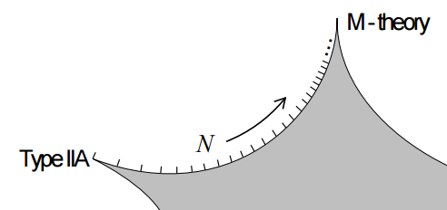
This may be thought of as a super $L_\infty$-theoretic incarnation of D0-brane condensation (Polchinski 99, around p. 8).

More in detail, if we distinguish $\overline{\psi} \wedge \Gamma_{10} \psi$ as an element of $\mathbb{R}^{9,1\vert \mathbf{16}+ \overline{\mathbf{16}^\ast}}$ or as the element $\mu_{D0}$ of $\mathfrak{string}_{IIA}$ (which in components are the same, just regarded in different contexts), then the relation between the D0-brane and the M-theory spacetime extension may be stated as follows: The following diagram is homotopy Cartesian (a homotopy pullback) square:

$$\array{ \mathbb{R}^{10,1\vert \mathbf{32}} &\longleftarrow& \mathfrak{d}0\mathfrak{brane} \\ \downarrow &(pb)& \downarrow \\ \mathbb{R}^{9,1\vert \mathbf{16}+ \mathbf{16}^\ast } &\longleftarrow& \mathfrak{string}_{IIA} } \,.$$

Remark

(brane intersection laws)

In addition to reflecting all the brane speciees, the above brane bouquet knows the brane intersection laws: there is a morphism $p_2\mathfrak{brane} \longrightarrow p_1 \mathfrak{brane}$ precisely if the given species of $p_1$-branes may end on the given species of $p_2$-branes (more discussion of this is in Fiorenza-Sati-Schreiber 13, section 3).

But recall from prop. the interpretation of the extended super Minkowski spacetimes as containing a condensate of branes sourcing the gauge field on the worldvolume of the branes that they may end on.

In conclusion this shows that given a cocycle $\mu_{p_1+2}$ for some super $p_1$-brane species inducing an extended super Minkowski spacetime via its homotopy fiber and then given a consecutive cocycle $\mu_{p_2+2}$ for a $p_2$-brane species on that homotopy fiber then $p_1$-branes may end on $p_2$-branes and the $p_2$-branes propagating in the extended spacetime $p_1 \mathfrak{brane}$ see a higher gauge field on their worldvolume of the kind sourced by boundaries of $p_1$-branes.

$\,$

$$\array{ { \text{spacetime} \atop \text{with}\,p_1\text{-brane condensate} } &&& p_1 \mathfrak{brane} &\overset{\mu_{p_2+2}}{\longrightarrow}& B^{p_2+2} \\ &&& {}^{\mathllap{hofib(\mu_{p_1+2})}}\downarrow \\ \text{spacetime} &&& \mathbb{R}^{d-1,1\vert \mathbf{N}} &\underset{\mu_{p_1+2}}{\longrightarrow}& B^{p_1+1}\mathbb{R} }$$

$\,$

Hence the extended super Minkowski spacetime $p_1 \mathfrak{brane}$ is like the original super spacetime $\mathbb{R}^{d-1,1\vert \mathbf{N}}$ but filled with a condensate of $p_1$-branes whose boundaries source a higher gauge field.

$\,$

While this is good, it means that at each stage of the brane bouquet we are describing $p_2$-brane dynamics on a fixed $p_1$-brane background field. But more generally we would like to describe the joint dynamics of all brane species at once.

$\,$

This we turn to now.

$\,$

Fields

In the discussion above we discovered all the p-brane species of string theory/M-theory, but each separately as a $b^{p+1}\mathbb{R}$-valued super $L_\infty$-cocycle on some extended super Minkowski spacetime classified by a previous cocycle.

Here we discuss that all these cocycles unify into single cocycles. However, these unified cocycles are no longer in ordinary cohomology, meaning that they no longer have coefficients in the simple line Lie-n algebras $b^{p+1}\mathbb{R}$ as in proposition .

Instead they have coefficients in richer and in general non-abelian L-∞ algebras. One says they are cocycles in non-abelian cohomology theory. By a phenomenon that has been called the Whitehead principle of non-abelian cohomology, this means more concretely that these unified cocycles are in a twisted generalized (Eilenberg-Steenrod) cohomology theory. Command of the general concept of this name is not strictly necessary for the analysis of the brane cocycles below, but a rough idea of its basic ingredients will make the meaning of the constructions and results very transparent. Therefore we start below with a lightning overview of the idea

• Twisted generalized cohomology

Since generalized cohomology is generally exhibited by classifying spaces, specifically topological spaces, to make use of these concepts we need a way to regard L-∞ algebras as certain spaces (or rather as homotopy types of certain spaces). This connection is provided by a theory called rational homotopy theory. Again, this is not strictly necessary for the derivation of the unified brane cocycles below, but it serves to greatly clarify the resulting structures. Therefore we next give a lightning survey of

• Rational homotopy theory.

After these conceptual preliminaries, we then turn to the concrete example of the brane bouquet established above and ask for homotopy descent of consecutive ordinary cocycles on extended super Minkowski spacetimes to single but twisted generalized cocycles down on plain super Minkowski spacetimes.

First we consider this for the D-branes and we derive that the unified F1/Dp-brane cocycles exist with coefficients the rationalization of twisted K-theory. This is the content of the section

• RR-Fields.

In direct analogy, we then discover the corresponding rationalized coefficients for the background fields for the M-branes. This turns out to be rationalized cohomotopy in degree 4. This we discuss in

• M-Flux Fields

More technically, what we show now is that there is homotopy descent of $p$-brane cocycles from extended super Minkowski spacetime down to ordinary super Minkowski spacetime which yields cocycles in twisted cohomology for the RR-field and the M-flux fields (Fiorenza-Sati-Schreiber 15, 16a).

$\,$

Twisted generalized cohomology

There is a traditional physics story for how twisted generalized (Eilenberg-Steenrod) cohomology appears on D-branes. Eventually we are after a precise derivation of this phenomenon from “first principles”, but as motivation and for intuition, it serves to recall the folklore:

It is often stated that a Chan-Paton gauge field on $n$ coincident D-branes is an SU(n)-vector bundle $V$, hence a cocycle in nonabelian cohomology in degree 1.

But this is not quite true. In general there are $n$ D-branes and $n'$ anti-D-branes coinciding, carrying Chan-Paton gauge fields $V_{brane}$ (of rank $n$) and $V_{\text{anti-brane}}$ (of rank $n'$), respectively, yielding a pair of vector bundles

$$(V_{\text{brane}}, V_{\text{anti-brane}}) \,.$$

Such pairs are also called virtual vector bundles.

But D-branes annihilate with anti-D-branes (Sen 98) when they are coincident and have exact opposite D-brane charge, which here means that they carry the same Chan-Paton vector bundle. In other words, pairs as above of the special form $(W,W)$ are equivalent to pairs of the form $(0,0)$.

$$(W,W) \;\sim\; 0 \,.$$

Hence the net Chan-Paton charge of coincident branes and anti-branes is really the equivalence class of $(V_{\text{brane}}, V_{\text{anti-brane}})$ under the equivalence relation which is generated by the relation

$$(V_{\text{brane}} \oplus W\,,\; V_{\text{anti-brane}} \oplus W) \;\sim\; (V_{brane}\,,\; V_{anti-brane})$$

for all complex vector bundles $W$ (Witten 98, Witten 00).

$\,$

The additive abelian group of such equivalence classes of virtual vector bundles is called topological K-theory. This behaves in many ways as ordinary cohomology does, but is richer. One says that it is ageneralized cohomology theory.

Hence by this story, D-brane charge should take values in twisted K-theory. Therefore, by the analog of the Maxwell equations for RR-fields, where D-brane charge plays the role of electric charge and magnetic charge in electromagnetism also the RR-fields must be cocycles in twisted K-theory (Moore-Witten 00).

$\,$

A famous fact about ordinary cohomology $H^n(X,\mathbb{Z})$ is that it is represented by topological spaces denoted $K(\mathbb{Z},n)$ or $B^n \mathbb{Z}$ and called Eilenberg-MacLane spaces: For $X$ a paracompact topological space then there is a natural bijection

$$H^n(X,\mathbb{Z}) \;\simeq\; \left\{ X \;\longrightarrow\; B^n \mathbb{Z} \right\}_{/homotopy}$$

between cohomology classes of $X$ and homotopy classes of continuous maps from $X$ to the Eilenberg-MacLane space. (This turns out to uniquely characterize the spaces $B^n \mathbb{Z}$.)

The collection of all these Eilenberg-MacLane spaces $B^n \mathbb{Z}$, as $n$ ranges, has the property that each is the based loop space of the previous one, up to weak homotopy equivalence

$$B^n \mathbb{Z} \underoverset{\text{weak hom. equivalence}}{\simeq}{\longrightarrow} \Omega_\ast \left( B^{n+1}\mathbb{Z} \right) \,.$$

More generally, in algebraic topology any sequence of pointed topological spaces $E_n$ indexed by the natural numbers and equipped with such weak homotopy equivalences

$$E_n \overset{\simeq}{\longrightarrow} \Omega_\ast \left( E_{n+1} \right)$$

is called a spectrum, or specifically an Omega-spectrum. See at geometry of physics – stable homotopy types for more on this.

Here for $X$ any pointed topological space, $\Omega X$ denotes the operation of constructing the space of continuous loops in $X$, starting and ending at the given basepoint. For later use we mention that a fancy-looking but most useful alternative way to think of a such as loop is as a homotopy from the basepoint to itself. Thought of this way, then the based loop space is equivalently the homotopy fiber product of the base point inclusion with itself, denoted as follows:

$$\Omega_\ast \left( X \right) \;\simeq\; \underset{ \text{homotopy} \atop \text{fiber product} }{ \underbrace{ \ast \underoverset{X}{h}{\times} \ast } } \,.$$

In direct analogy to the above situation, one says for $E_\bullet$ any such Omega-spectrum that the homotopy classes of continuous maps into its component space in degree $n$

$$E^n(X) \;\coloneqq\; \left\{ X \longrightarrow E_n \right\}_{/\text{homotopy}}$$

are the $E$-generalized cohomology classes of $X$ i degree $n$.

One also says that the cohomology theory $E^\bullet(-)$ is generalized cohomology theory is represented by the spectrum $E$.

The example of interest for D-brane charge, topological K-theory, is the generalized cohomology theory denoted by

$$E = KU$$

with

$$KU_{2n} \simeq (B U) \times \mathbb{Z} \;\;\,,\;\; KU_{2n+1} \simeq U$$

where

1. $U$ denotes the stable unitary group,

2. $B U$ denotes the classifying space for complex vector bundles.

So in this case a cocycle is represented by the homotopy class of a map of the form

$$\left(V_{brane}, n_{\text{anti-brane}} \right) \;\colon\; X \overset{}{\longrightarrow} (B U) \times \mathbb{Z}$$

which gives a complex vector bundle $V_{\text{brane}}$ and the trivial vector bundle $\mathbb{C}^{n_{\text{anti-brane}}}$ of rank $n_{\text{anti-brane}}$, hence a virtual vector bundle of the form

$$(V_{\text{brane}}, \mathbb{C}^{n_{\text{anti-brane}}}) \,.$$

A basic fact proven in topological K-theory is that the K-theory class of every virtual vector bundle is represented by one of this form, and it is in this way that $KU_0 = (B U) \times \mathbb{Z}$ is the coefficient space for topological K-theory.

But this is not yet the full story: Above we saw that the Chan-Paton gauge field on a D-brane is actually a twisted vector bundle with twist given by the Kalb-Ramond B-field sourced by a string condensate. (Freed-Witten anomaly cancellation).

Such twisted generalized cohomology is given by generalizing the above concept of Omega-spectra by allowing the base point $\ast$ to become a classifying space of twists. The result is called a parameterized spectrum. Such consists of:

1. a classifying space of twists $B G$

2. a spectrum object in the slice category $Top_{/B G}$, namely a sequence of spaces, denoted $E_n/G$, equipped with maps

   $$id \;\colon\; B G \to E_n/G \to B G$$

   and weak homotopy equivalences from the $n$th space to the homotopy fiber product of space inclusion of the space of twists with itself:

   $$E_n/G \overset{\phantom{AA}\simeq\phantom{AA} }{\longrightarrow} \Omega_{B G} (E_{n+1}/G) \coloneqq \underset{\text{homotopy} \atop {\text{fiber} \atop \text{product} } }{\underbrace{ B G \underoverset{E_{n+1}/G}{h}{\times} B G }}$$

To get a feeling for this definition, consider two extremal cases of parameterized spectra:

1. An ordinary spectrum $E$ is a parameterized spectrum over the point (i.e. no twists);

   $$\array{ E \\ \downarrow \\ \ast }$$

2. An ordinary topological space $X$ is identified with the zero-spectrum parameterized over $X$, which is just

   $$\array{ X \\ \downarrow^{\mathrlap{id}} \\ X }$$

Hence a general parameterized spectrum interpolates between these two extremes, it combines the non-abelian cohomology represented by topological spaces such as $B U$ with the abelian cohomology represented by spectra:

More in detail, given a parameterized spectrum $E$ over $B G$, then we have the following elegant picture of twisted $E$-cohomology (NSS 12, section 4.1):

1. A twist $\tau$ for the $E$-cohomology of some topological space $X$ is a map

   $$\array{ X \\ & {}_{\mathllap{\tau}}\searrow \\ && B G }$$

   from $X$ to the spectrum’s classifying space of twists.

2. The $\tau$-twisted $E$-cohomology of $X$ in degree $n$ is the set of homotopy classes of maps $X \overset{\phi}{\longrightarrow} E_n/G$ together with a homotopy $p_n \circ \phi \simeq \tau$:

   $$E^{n+\tau}(X) \;\coloneqq\; \left\{ \array{ X && \longrightarrow && E_n/G \\ & {}_{\mathllap{\tau}} \searrow && \swarrow_{\mathrlap{p_n}} \\ && B G } \right\}_{/\text{homotopy}}$$

3. There is a homotopy fiber sequence (in parameterized spectra)

   $$\array{ E &\longrightarrow& E/G \\ && \downarrow \\ && B G }$$

   and this equivalently exhibits $E/G$ as the homotopy quotient of an ordinary spectrum $E$ by a

coherent homotopy action of $G$.

We now translate this situation from topological spaces to super L-∞ algebras via the central theorem of rational homotopy theory, which we now recall.

$\,$

Rational homotopy theory

Recall from the discussion above that an L-∞ algebra $\mathfrak{g}$ may be thought of as a Lie algebra “up to coherent higher homotopy”: with the unary bracket $[-]$ regarded as a differential $\partial \coloneqq [-]$, then for instance the trinary bracket is a chain homotopy up to which the Jacobi identity holds

$$[x,[y,z]] \underoverset{\simeq}{\partial [x,y,z]}{\longrightarrow} [[x,y],z] \pm [y,[x,z]] \,.$$

In direct analogy, for $X$ any pointed topological space, then the based loop space $\Omega_\ast(X)$ (the topological space whose elements are continuous paths from the basepoint to itself) naturally is a group “up to coherent higher homotopy”.

Namely

• the operation of concatenating two loops $\alpha,\beta \colon [0,1] \to X$ to a new loop

  $$[0,1] \overset{2 \cdot(-)}{\longrightarrow} [0,2] \overset{}{\longrightarrow} X$$

  gives it the structure of a semi-group whose associativity law holds up to homotopy;

• the constant loop gives it the structure of a monoid up to coherent homotopy, called an A-∞ space

• the reversal of loops

  $$[0,1] \overset{1-(-)}{\longrightarrow} [0,1] \overset{\alpha}{\longrightarrow} X$$

  finally gives it inverses up to homotopy and makes it what is called a a grouplike A-∞ space or ∞-group for short.

Conversely, for $G$ any ∞-group then there is an essentially unique connected space $B G$ with $G \;\simeq\; \Omega B G$ (the May recognition theorem).

Now in a similar manner, every double loop space $\Omega_\ast(\Omega_\ast(X))$ becomes a “first order abelian” ∞-group by exchanging loop directons. This may be called a braided ∞-group,

$\,$

Hence for $G$ a braided ∞-group then $B G$ is itself an ∞-group and so there exists an essentially unique simply connected space

$$B^2 G \coloneqq B (B G)$$

with

$$G \;\simeq\; \Omega^2 B^2 G \,.$$

$\,$

And so forth:

Every triple loop space $\Omega^3 X$

becomes a “second order abelian” ∞-group

by exchanging loop directons

called a sylleptic ∞-group.

etc.

$\,$

In a spectrum $E$,

the maps $E_n \stackrel{\simeq}{\to} \Omega E_{n+1}$

exhbit $E_0$ as an infinite loop space

hence as a fully abelian ∞-group.

$\,$

It turns out that by a homotopy theoretic version of Lie theory,

there is an L-∞ algebra $\mathfrak{g}$ associated with any ∞-group

$$\mathfrak{g} \simeq \mathfrak{l} B G \,.$$

or

$$B\mathfrak{g} \simeq \mathfrak{l} B^2 G$$

etc.

$\,$

Its Chevalley-Eilenberg algebra $CE(\mathfrak{B g})$

is called a Sullivan model for $B^2 G$.

$\,$

For example the $L_\infty$-algebra associated with an Eilenberg-MacLane space

$$K(\mathbb{Z},n+1) \simeq B^{n+1}\mathbb{Z}$$

is the line Lie-n algebra from above:

$$\mathfrak{l}(B^{n+1} \mathbb{Z}) \;\simeq\; B^n \mathbb{R} \,.$$

$\,$

The main theorem of rational homotopy theory (Quillen 69, Sullivan 77)

says that the L-∞ algebra $\mathfrak{l}(B^2 G)$ equivalently reflects the rationalization of $B^2 G$

(in fact the real-ification, since we are considering $L_\infty$-algebras over the real numbers).

This means that weak equivalence between $L_\infty$-algebras correspond to maps between spaces

that induce isomorphism on real-ified homotopy groups

$$\left\{ \;\;\;\;\; \array{ B^2 G_1 \overset{\phantom{AA}f\phantom{AA}}{\longrightarrow} B^2 G_2 \\ \text{such that:} \\ \pi_\bullet(B^2 G_1)\otimes_{\mathbb{Z}} \mathbb{R} \underoverset{\simeq}{\pi_\bullet(f) \otimes_{\mathbb{Z}} \mathbb{R} }{\longrightarrow} \pi_\bullet(B^2 G_2) \otimes_{\mathbb{Z}} \mathbb{R} } \;\;\;\;\; \right\} \;\;\;\leftrightarrow\;\;\; \left\{ \; \mathfrak{l}(B^2 G_1) \stackrel{\simeq}{\longrightarrow} \mathfrak{l}(B^2 G_2) \; \right\} \,.$$

For concise review in the language that we use here see Buijs-Félix-Murillo 12, section 2.

$\,$

We apply this rational homotopy theory functor

$$\mathfrak{l}(-) \;\colon\; \text{Spaces} \longrightarrow L_\infty\text{-Algebras}$$

to find the $L_\infty$-algebraic version of parameterized spectra

hence of twisted cohomology:

$\,$

$$\array{ { \text{parameterized} \atop \text{spectrum} } \;\;\;&\;\;\;\; \left\{ \array{ id : B^2 G \to E_n/ B G \to B^2 G \\ E_n/ B G \stackrel{\simeq}{\longrightarrow} \Omega_{B^2 G} (E_{n+1}/ B G) } \right\} \;&\;\leftrightarrow\;&\; \left( \array{ E &\longrightarrow& E/B G \\ && \downarrow \\ && B^2 G } \right) \\ & \mathfrak{l}(-)\downarrow \\ L_\infty\text{Algebra} \;\;\;&\;\;\;\; \left\{ \array{ id : \mathfrak{l}(B^2 G) \to \mathfrak{l}(E_n/ B G) \to \mathfrak{l}(B^2 G) \\ \mathfrak{l}(E_n/ B G) \stackrel{\simeq}{\longrightarrow} \Omega_{\mathfrak{l}(B^2 G)} \mathfrak{l}(E_{n+1}/ B G) } \right\} \;&\;\leftrightarrow\;&\; \left( \array{ V[1] &\longrightarrow& V[1]/\mathfrak{g} \\ && \downarrow \\ && B \mathfrak{g} } \right) }$$

$\,$

Here $V \simeq E \otimes \mathbb{R}$ is a chain complex

underlying the real-ification of the spectrum $E$

(stable Dold-Kan correspondence).

$\,$

So for $\mathbb{R}^{d-1,1\vert \mathbf{N}}$ some super Minkowski spacetime, a cocycle in $\mathfrak{g}$-twisted $V$-cohomology is a diagram of the form

$$\array{ \mathbb{R}^{d-1,1\vert \mathbf{N}} && \overset{}{\longrightarrow} && V/\mathfrak{g} \\ & \searrow && \swarrow \\ && B \mathfrak{g} }$$

$\,$

Now given one stage in the brane bouquet

$$\array{ \widehat{\widehat{\mathfrak{g}}} \\ {}^{\mathllap{hofib(\mu_{p_2})}}\downarrow \\ \hat \mathfrak{g} & \stackrel{\mu_{p_2}}{\longrightarrow} & B\mathfrak{h}_2 \\ {}^{\mathllap{hofib(\mu_{p_1})}}\downarrow \\ \mathfrak{g} &\overset{\mu_{p_1}}{\longrightarrow}& B\mathfrak{h}_1 }$$

we want to descent $\mu_{p_2}$ to $\mathfrak{g}$.

$\,$

By the general theory of principal ∞-bundles (Nikolaus-Schreiber-Stevenson 12):

1. $\widehat{\mathfrak{g}}$ has a $\mathfrak{h}_1$-∞-action

2. equipping $B \mathfrak{h}_2$ with an $\mathfrak{h}_1$-∞-action

   is equivalent to finding a homotopy fiber sequence as on the right here:

   $$\array{ \hat \mathfrak{g} && \stackrel{\mu_2}{\longrightarrow} && \mathbf{B}\mathfrak{h}_2 \\ {}^{\mathllap{hofib(\mu_1)}}\downarrow && && \downarrow^{\mathrlap{hofib(p_\rho)}} \\ \mathfrak{g} && && (\mathbf{B}\mathfrak{h}_2)/\mathfrak{h}_1 \\ & {}_{\mathllap{\mu_1}}\searrow && \swarrow_{\mathrlap{p_\rho}} \\ && \mathbf{B}\mathfrak{h}_1 } \,.$$

3. $\mu_2$ is $\mathfrak{h}_1$-equivariant precisely if it descends to a morphism

   $$\mu_2/\mathfrak{h}_1 \;\colon\; \mathfrak{g} \longrightarrow (\mathbf{B}\mathfrak{h}_2)/\mathfrak{h}_1$$

   such that this diagram commute up to homotopy:

   $$\array{ \hat \mathfrak{g} && \stackrel{\mu_2}{\longrightarrow} && \mathbf{B}\mathfrak{h}_2 \\ {}^{\mathllap{hofib(\mu_1)}}\downarrow && && \downarrow^{\mathrlap{hofib(p_\rho)}} \\ \mathfrak{g} && \stackrel{\mu_2/\mathfrak{h}_1}{\longrightarrow} && (\mathbf{B}\mathfrak{h}_2)/\mathfrak{h}_1 \\ & {}_{\mathllap{\mu_1}}\searrow && \swarrow_{\mathrlap{p_\rho}} \\ && \mathbf{B}\mathfrak{h}_1 } \,.$$

4. if so, then resulting triangle diagram

   $$\array{ \mathfrak{g} && \stackrel{\mu_2/\mathfrak{h}_1}{\longrightarrow} && (\mathbf{B}\mathfrak{h}_2)/\mathfrak{h}_1 \\ & {}_{\mathllap{\mu_1}}\searrow && \swarrow_{\mathrlap{p_\rho}} \\ && \mathbf{B}\mathfrak{h}_1 }$$

   exhibits $\mu_2/\mathfrak{h}_1$ as a cocycle in (rational) $\mu_1$-twisted cohomology

   with respect to the local coefficient bundle $p_\rho$.

$\,$

We now work out this general prescription

for the cocycles in the brane bouquet.

$\,$

RR-fields

$\,$

By the brane bouquet above

the type IIA D-branes

are given by super $L_\infty$ cocycles of the form

$$\mathfrak{string}_{IIA } \overset{\mu_{Dp}}{\longrightarrow} B^{p+1}\mathbb{R}$$

for $p \in \{0,2,4,6,8,10\}$.

$\,$

Notice that

$$H^\bullet(B U, \mathbb{Z})$$

has one generator in each even degree, the universal Chern classes.

Hence the $L_\infty$-algebra

$$\mathfrak{l}(KU)$$

is given by

$$CE(\mathfrak{l}(KU)) \;\simeq\; \left\{ d \omega_{2p+2} = 0 \;\vert\; p \in \mathbb{Z} \right\} \,.$$

This allows to unify the D-brane cocycles

into a single morphism of super $L_\infty$-algebras of the form

$$\array{ \mathfrak{string}_{IIA} && \stackrel{\phantom{AA}\mu_D\phantom{AA}}{\longrightarrow} && \mathfrak{l}(KU) \\ {}^{\mathllap{hofib(\mu_{F1})}}\downarrow \\ \mathbb{R}^{9,1\vert \mathbf{16}+ \overline{\mathbf{16}}} \\ & {}_{\mathllap{\mu_{F1}}}\searrow \\ && \mathbf{B}^2 \mathbb{R} } \,.$$

$\,$

By the above prescription, descending $\mu_D$ is equivalent

to finding a commuting diagram in the homotopy category of super $L_\infty$-algebras

of the form

$$\array{ \mathfrak{string}_{IIA} && \stackrel{\phantom{AA}\mu_D\phantom{AA}}{\longrightarrow} && \mathfrak{l}(KU) \\ {}^{\mathllap{hofib(\mu_{F1})}}\downarrow && && \downarrow^{\mathrlap{hofib(\phi)}} \\ \mathbb{R}^{9,1\vert \mathbf{16}+ \overline{\mathbf{16}}} &&\overset{\phantom{AA}\mu_{D}/B \mathbb{R}\phantom{AA} }{\longrightarrow}&& \text{something} \\ & {}_{\mathllap{\mu_{F1}}}\searrow && \swarrow_{\mathrlap{\phi}} \\ && \mathbf{B}^2 \mathbb{R} } \,.$$

$\,$

This turns out to exist as follows (Fiorenza-Sati-Schreiber 16a, section 5):

Define the $L_\infty$-algebra

$$\mathfrak{l}(KU / BU(1))$$

by

$$CE\left(\mathfrak{l}(KU / BU(1))\right) \;=\; \left\{ \array{ d h_3 = 0\;,\; \\ d \omega_{2p+2} = h_3 \wedge \omega_{2p} } \right\} \,.$$

Moreover write

$$\mathbb{R}^{9,1\vert \mathbf{16} + \overline{\mathbf{16}}}_{res}$$

for the super $L_\infty$-algebra whose Chevalley-Eilenberg algebra is

$$CE\left( \mathbb{R}^{9,1\vert \mathbf{16} + \overline{\mathbf{16}}}_{res} \right)[f_2,h_3]/(d f_2 = \mu_{F1} + h_3)$$

$\,$

Proposition

(Fiorenza-Sati-Schreiber 16a, theorem 4.16)

The super $L_\infty$-algebra $\mathbb{R}^{9,1\vert \mathbf{16} + \overline{\mathbf{16}}}_{res}$

is a resolution of type IIA super-Minkowski spacetime.

in that there is a weak equivalence

$$\mathbb{R}^{9,1\vert \mathbf{16} + \overline{\mathbf{16}}}_{res} \stackrel{\phantom{AA}\simeq\phantom{AA}}{\longrightarrow} \mathbb{R}^{9,1\vert \mathbf{16} + \overline{\mathbf{16}}} \,.$$

This fits into a commuting diagram of the form

$$\array{ \left\{ {{d e^a = \overline{\psi}\Gamma^a \wedge \psi } \atop {d \psi^\alpha = 0}} \atop { d f_2 = \mu_{F1}} \right\} && \mathfrak{string}_{IIA} && \stackrel{ \mu_D }{\longrightarrow} && \mathfrak{l}(KU) && \left\{ d \omega_{2 p+2} = 0 \right\} \\ && \downarrow^{\mathrlap{hofib(\mu_{F1})}} && && \downarrow^{\mathrlap{\phi}} \\ \left\{ {{d e^a = \overline{\psi}\Gamma^a \wedge \psi } \atop {d \psi^\alpha = 0}} \atop { d f_2 = \mu_{F1} + h_3 } \right\} & & \mathbb{R}_{res}^{9,1\vert \mathbf{16}+ \overline{\mathbf{16}}} && \stackrel{ \mu_{F1/D} }{\longrightarrow} && \mathfrak{l}(KU / B U(1)) && \left\{ d\omega_{2p+2} = h_3\wedge \omega_{2p} \right\} \\ && & {}_{\mathllap{\mu_{F 1}}}\searrow && \swarrow_{\mathrlap{\phi}} \\ && && \mathbf{B}^2 \mathbb{R} \\ && && \left\{ d h_3 = 0 \right\} } \,.$$

$\,$

In conclusion

$\;\;$the type IIA F1-brane and D-brane cocycles with $\mathbb{R}$-coefficients

$\;\;$do descent to super-Minkowski spacetime

$\;\;$as one single cocycle with coefficients

$\;\;$in rationalized twisted K-theory.

$\,$

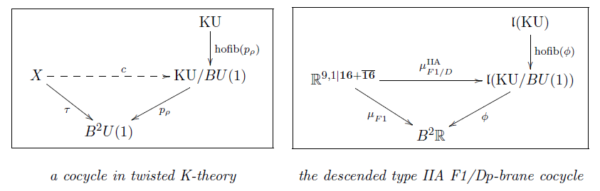
M-flux fields

$\,$

The part of the brane bouquet giving the M-branes is

$$\array{ \mathfrak{m}2\mathfrak{brane} &\stackrel{\mu_{M5}}{\longrightarrow}& \mathbf{B}^6 \mathbb{R} \\ {}^{\mathllap{hofib(\mu_{M2})}}\downarrow \\ \mathbb{R}^{10,1\vert \mathbf{32}} & \stackrel{\mu_{M2}}{\longrightarrow} & \mathbf{B}^3 \mathbb{R} \\ {}^{\mathllap{hofib(\mu_{D 0})}}\downarrow \\ \mathbb{R}^{9,1\vert \mathbf{16} + \overline{\mathbf{16}}} }$$

$\,$

In order to descend this, consider the $L_\infty$-algebra corresponding to the 4-sphere

$$\mathfrak{l}(S^4) \,.$$

By standard results on rational n-spheres, this is given by

$$CE(\mathfrak{l}S^4) \;\simeq\; \left\{ \array{ d \, g_4 = 0\,,\, \\ d\, g_7 + \tfrac{1}{2} g_4 \wedge _4 = 0 } \right\} \,.$$

(…)

Definition

For $p \in \mathbb{N}_{even}$, write

$b^{2p+2} \mathbb{R}/b^p \mathbb{R}$ for the L-∞ algebra given by the Chevalley-Eilenberg algebra

$$CE(b^{2p+2} \mathbb{R}/b^p \mathbb{R}) = \left(\left\langle g_{p+2}, g_{2p+3}\right\rangle), {{d g_{p+2} = 0} \atop {d g_{2p+3} = g_{p+2} \wedge g_{p+2}}}\right) \,.$$

Remark

Regarded as a Sullivan model in rational homotopy theory, then the dg-algebra of def. is a minimal model for the rationalization of the $(p+2)$-sphere.

By the recognition theorem for L-∞ extensions we get:

Proposition

For $p \in \mathbb{N}_{even}$, there is a homotopy fiber sequence in the homotopy theory of L-∞ algebras of the form

$$\array{ b^{2p+2} \mathbb{R} \\ \downarrow \\ b^{2p+2} \mathbb{R}/b^{p}\mathbb{R} &\stackrel{}{\longrightarrow}& b^{p+1}\mathbb{R} }$$

where on formal dual Chevalley-Eilenberg algebras in terms of our defining generating elements the horizontal map is given by $g_{p+4}\mapsto g_{p+4}$ and the vertical map by $g_{p+4}\mapsto 0$ and $g_{2p+3}\mapsto g_{2p+3}$.

By the discussion at ∞-action this exhibits a $b^{p}\mathbb{R}$-action on $b^{2p+2}\mathbb{R}$, for which $b^{2p+2} \mathbb{R}/b^{p}\mathbb{R}$ is the homotopy quotient, whence the notation.

Example

For $p=2$ and regarded as a statement in rational homotopy theory via remark , then the extension in prop. is a Sullivan minimal model for the rationalized Hopf fibration

$$\array{ S^3 &\longrightarrow& S^7 \\ && \downarrow \\ && S^4 }$$

But since $\mathfrak{m}2\mathfrak{brane}$ is a $b^2 \mathbb{R}$-principal ∞-bundle, it is natural to ask whether $h_3 \wedge \mu_4 + \frac{1}{15} \mu_7$ is $b^2 \mathbb{R}$-equivariant with respect to some natural $b^2\mathbb{R}$-∞-action on $b^6 \mathbb{R}$. Such a natural action is given by prop. . To exhibit in components the equivariance of the 7-cocycle in corollary with respect to this action we need a resolution of super Minkowski spacetime:

Definition

Write $\mathbb{R}_{res}^{10,1\vert \mathbf{32}}$ for the super L-∞ algebra whose Chevalley-Eilenberg algebra is obtained from that of super Minkowski spacetime by

$$CE\left( \mathbb{R}_{res}^{10,1\vert \mathbf{32}} \right) \coloneqq \left( CE\left( \mathbb{R}^{10,1\vert \mathbf{32}}\right)\otimes \left\langle h_3, g_4\right\rangle , {{d h_3 = g_4 - \mu_4} \atop {d g_4 = 0}} \right) \,.$$

Proposition

The canonical morphism

$$\mathbb{R}_{res}^{10,1\vert \mathbf{32}} \stackrel{\simeq}{\longrightarrow} \mathbb{R}^{10,1\vert \mathbf{32}}$$

given dually by $\psi^\alpha \mapsto \psi^\alpha$, $e^a \mapsto e^a$, is an equivalence of $L_\infty$-algebras. It factors the morphism $\mathfrak{m}2\mathfrak{brane} \longrightarrow \mathbb{R}^{10,1\vert \mathbf{32}}$ from def. through a morphism $\mathfrak{m}2\mathfrak{brane} \longrightarrow \mathbb{R}^{10,1\vert \mathbf{32}}_{res}$ which on formal dual CE-elements is given by $h_3 \mapsto 0$, $g_4 \mapsto 0$ and by being the identity on all other generators.

Proposition

There is a diagram of L-∞ algebras of the form

$$\array{ && \vdots && && \vdots \\ && \downarrow \downarrow && && \downarrow \downarrow \\ && \mathfrak{m}2\mathfrak{brane} && \stackrel{h_3 \wedge \mu_4 + \frac{1}{15}\mu_7 }{\longrightarrow} && b^6 \mathbb{R} \\ && \downarrow && && \downarrow \\ \mathbb{R}^{10,1\vert\mathbf{32}} &\stackrel{\simeq}{\longleftarrow}& \mathbb{R}_{res}^{10,1\vert\mathbf{32}} && \stackrel{h_3 \wedge (g_4 + \mu_4) + \frac{1}{15}\mu_7 }{\longrightarrow} && b^6 \mathbb{R}/b^2 \mathbb{R} \\ && & {}_{\mathllap{}}\searrow && \swarrow \\ && && b^3 \mathbb{R} }$$

Proof

That the diagram exists and commutes at the level of the underlying graded algebras of the formal dual CE-algebras is immediate in terms of the defining generators: each generator is mapped to the generator of the same name, if present, in the codomain, or to zero otherwise, except for $g_7 \in CE(b^6 \mathbb{R})$ which is sent to $h_3 \wedge \mu_4 + \frac{1}{15}\mu_7$ and $g_7 \in CE(b^6 \mathbb{R}/b^2 \mathbb{R})$, which is sent to $h_3 \wedge (g_4 + \mu_4) + \frac{1}{15}\mu_7$, as indicated.

It remains to check that the middle horizontal map respects the CE-differentials: by prop. we have

$$\begin{aligned} d(h_3 \wedge (g_4 + \mu_4) + \frac{1}{15}\mu_7) &= (g_4 - \mu_4) \wedge (g_4 + \mu_4) + \mu_4 \wedge \mu_4 \\ & = g_4 \wedge g_4 \end{aligned}$$

and by def. this says indeed that $g_7 \mapsto h_3 \wedge (g_4 + \mu_4) + \frac{1}{15}\mu_7$ respects the CE-differentials.

Remark

The form of the equivariant cocycle in prop. is that of the curvature of the WZW term of the sigma model describing the M5-brane as considered in (BLNPST 97, (6),(8)).

Remark

In view of remark , prop. says that the CE-elements $\mu_4$ and $\mu_7$ of prop. define a cocycle with values in the rational 4-sphere. In the discussions in geometry of physics – WZW terms and geometry of physics – BPS charges we see that under Lie integration and globalization in higher Cartan geometry, these elements encode the supergravity C-field and its magnetic dual. That these fields should take values in the 4-sphere was first suggested in (Sati 13, section 2.5).

(…)

Proposition

Fiorenza-Sati-Schreiber 15, section 3

There is a homotopy fiber sequence of $L_\infty$-algebras as on the right

$$\left( \array{ && S^7 \\ && \downarrow \\ && S^4 \\ & \swarrow \\ B SU(2) \\ \downarrow^{\mathrlap{c_2}} \\ B^3 U(1) } \right) \;\; \stackrel{\phantom{AA}\mathfrak{l}(-)\phantom{AA} }{\mapsto} \;\; \left( \array{ && B^6 \mathbb{R} \\ && \downarrow^{\mathrlap{ hofib(\mathfrak{l}(c_2)) } } \\ &&\mathfrak{l}(S^4) \\ & \swarrow_{\mathfrak{l}(c_2)} \\ B^3 \mathbb{R} } \;\;\;\;\;\;\;\;\;\;\;\;\;\;\;\; \right)$$

which is the image under $\mathfrak{l}(-)$ of the quaternionic Hopf fibration.

This makes a commuting diagram

in the homotopy category of super $L_\infty$-algebas

of the form

$$\array{ \left\{ { { d e^a = \overline{\psi}\wedge \Gamma^a \wedge \psi } \atop { d \psi^\alpha = 0 } } \atop d h_3 = - \mu_{M2} \right\} && \mathfrak{m}2\mathfrak{brane} && \stackrel{ \mu_{M5} }{\longrightarrow} && B^6 \mathbb{R} && \left\{ d g_7 = 0 \right\} \\ && \downarrow^{\mathrlap{hofib(\mu_{M2})}} && && \downarrow^{\mathrlap{hofib(\mathfrak{l}(c_2))}} \\ \left\{ { { d e^a = \overline{\psi}\wedge \Gamma^a \wedge \psi } \atop { d \psi^\alpha = 0 } } \atop d h_3 = g_4 - \mu_{M2} \right\} && \mathbb{R}_{res}^{10,1\vert\mathbf{32}} && \stackrel{ \mu_{M2/M5} }{\longrightarrow} && \mathfrak{l} S^4 && \left\{ {d g_4 = 0} \atop {d g_7 + \tfrac{1}{2} g_4 \wedge g_4 = 0} \right\} \\ && & {}_{\mathllap{\mu_{M2}}}\searrow && \swarrow_{\mathrlap{\mathfrak{l}(c_2)}} \\ && && \mathbf{B}^3 \mathbb{R} \\ && && \left\{ d g_4 = 0\right\} }$$

In conclusion

$\;\;$this says that, rationally,

$\;\;$M2-brane charge is in degree-4 ordinary cohomology

$\;\;$and it twists M5-brane charge

$\;\;$which is, rationally, in unstable degree-4 cohomotopy.

$\,$

This confirms a conjecture due to

(Sati 10, section 6.3, Sati 13, section 2.5).

based on the observation that

the equations of motion of 11-dimensional supergravity

for the supergravity C-field field strength $G_4$ say that

$$d G_7 + \tfrac{1}{2} G_4 \wedge G_4 = 0$$

with $G_7 = \ast G_4$ the Hodge dual

and this is just the algebraic relation for the Sullivan model of the rational 4-sphere.

$\,$

Notice that, unstably, the 4-sphere

is just the space whose non-torsion homotopy groups

hence those that are visible in rational homotopy theory

are in degrees 2+2 and 5+2:

k	1	2	3	4	5	6	7
$\phantom{AA}\pi_k(S^4)\phantom{AA}$	$\phantom{AA}0\phantom{AA}$	$\phantom{AA}0\phantom{AA}$	$\phantom{AA}0\phantom{AA}$	$\phantom{AA}\mathbb{Z}\phantom{AA}$	$\phantom{AA}\mathbb{Z}/2\phantom{AA}$	$\phantom{AA}\mathbb{Z}/2\phantom{AA}$	$\phantom{AA}\mathbb{Z} \oplus \mathbb{Z}/{12}\phantom{AA}$

$\,$

But the correct non-rational lift of the $\mathfrak{l}(S^4)$-coefficients

will also have to be such that it somehow gives rise to twisted K-theory

under (double) dimensional reduction. This is still an open problem.

For further comments see the talk

Equivariant cohomology of M2/M5-branes

$\,$

$\,$

Now that we have found

the descended $L_\infty$-cocycles

for all super $p$-branes

in twisted cohomology, rationally,

we may analyze their behaviour under double dimensional reduction

and discover the super $L_\infty$-algebraic incarnation

of various dualities in string theory.

$\,$

Double dimensional reduction

Underlying most of the dualities in string theory is the phenomenon of “double dimensional reduction” (Duff-Howe-Inami-Stelle 87), so called because:

1. the dimension of spacetimes is reduced by Kaluza-Klein compactification on a fiber $F$;

2. in parallel the dimension of branes is reduced if they wrap $F$.

We now explain a mathematical formulation of double dimensional reduction of brane charges, following (FSS 16b, section 3, BMSS 18, section 2.2):

First we give an exposition of the

• Idea.

Then we discuss a first approximation to a mathematical formalization:

• Via free looping (no 0-brane effect)

and then the accurate and fully general formalization in

• Via cyclification (with 0-brane effects)

We then specialize this general procedure to super L-infinity algebras so that it applies to the super $p$-brane cocycles in

• On super p-brane cocycles

$\,$

Idea

The original example of double dimensional reduction (Duff-Howe-Inami-Stelle 87) is supposed to underly the duality between M-theory and type IIA string theory. In this case

• spacetime$X_{11}$ is an 11d circle-fiber bundle locally of the form $X_{11} = X_{10} \times S^1$ over a 10d base spacetime;

• an M-theory membrane (M2-brane) with cyclindrical worldvolume

  $$\Sigma_3 = \Sigma_2 \times S^1$$

  wraps the circle fiber if its trajectory

  $$\phi_{M2} \;\colon\; \Sigma_3 \longrightarrow X_{11}$$

  is of the form

  $$\phi_{F1} \times \mathrm{id}_{S^1} \;\colon\; \Sigma_2 \times S^1 \longrightarrow X_{10} \times S^1 \,.$$

As the Riemannian circumference of the circle fiber $S^1$ tends towards zero this effectively looks like the 2-dimensional worldsheet $\Sigma_2$ of a string tracing out a trajectory in 10-dimensional spacetime:

$$\phi_{F1} \;\colon\; \Sigma_2 \longrightarrow X_{10}$$

$\,$

But there is also “single dimensional reduction” when the membrane does not wrap the fiber space:

$$\array{ \Sigma_3 && \overset{\phi_{M2}}{\longrightarrow} && X_{11} \\ & {}_{\phi_{D2}}\searrow && \nearrow \\ && X_{10} }$$

In this case it looks like a membrane in 10d spacetime, now called the D2-brane.

Similarly the M5-brane in M-theory

$$\phi_{M5} \;\colon\; \Sigma_{6} \longrightarrow X_{11}$$

may wrap the circle fiber to yield a 4-brane in 10d, called the D4-brane or it may not wrap the circle fiber to yield a 5-brane in 10d, called the NS5-brane.

$\,$

Beware the naive treatment of branes in this traditional argument. And even naively, this is not the full story yet: The $S^1$-fibration itself is supposed to re-incarnate in 10d as the D0-brane and the D6-brane.

Hence double dimensional reduction from M-theory to type IIA string theory is meant to, schematically, involve decompositions as follows

$$\underset{spacetime}{ \underbrace{ \array{ X_{11} \\ \downarrow^{\pi} \\ X_{10} } } } \;\; \underset{branes}{ \underbrace{ \array{ && && \text{M2-brane} && && && \text{M5-brane} \\ && & {}^{\mathllap{wrapped}}\swarrow && \searrow^{\mathrlap{not \atop wrapped}} & & && {}^{\mathllap{wrapped}}\swarrow && \searrow^{\mathrlap{not \atop wrapped}} \\ \text{D0-brane} && \text{F1-brane} && && \text{D2-brane} && \text{D4-brane} && && \text{NS5-brane} } } }$$

Above we saw that all super p-branes are characterized by the flux fields $H_{p+2}$ that they are charged under, more precisely by the bispinorial component of $H_{p+2}$ which is constrained to be super-tangent-space-wise the form

$$H_{p+2}^{fermionic} \;=\; \tfrac{i^{p(p-1)/2}}{p!} \, \left( \overline{\Psi} \wedge \Gamma_{a_1 \cdots a_p}\Psi \right) \wedge E^{a_1} \wedge \cdots \wedge E^{a_p}$$

where $(E^a, \Psi^\alpha)$ is the super vielbein (graviton and gravitino).

$\,$

Hence we will formalize double dimensional reduction in terms of these fields.

$\,$

Again there is a naive picture to help the intuition: Let $G_4 \in \Omega^4_{cl}(X_{11})$ be the differential 4-form flux field strength of the supergravity C-field.

Under the Gysin sequence for the spherical fibration

$$\array{ S^1 &\hookrightarrow& X_{11} \\ && \downarrow^{\mathrlap{\pi}} \\ && X_{10} }$$

this decomposes in cohomology as

$$G_4 = (d x^{10}) \wedge H_3 + \pi^\ast F_4$$

thus giving rise in 10d to

1. a 3-form $H_3$, the Kalb-Ramond B-field field strength that the string couples to;

2. a 4-form $F_4$, the RR-field field strength in degree 4, that the D2-brane couples to.

Similary the 7-form field strength $G_7$ decomposes as

$$G_7 = (d x^{10}) \wedge F_6 + \pi^\ast H_7$$

thus giving rise in 10d to

1. a 6-form $F_6$, the RR-field field strength in degree 6, that the D4-brane couples to

2. a 7-form $H_7$, the dual NS-NS field strength that the NS5-brane couples to.

$$\underset{spacetime}{ \underbrace{ \array{ X_{11} \\ \downarrow^{\pi} \\ X_{10} } } } \;\; \underset{fluxes}{ \underbrace{ \array{ && && G_4\text{-flux} && && && G_7\text{-flux} \\ && & {}^{\mathllap{wrapped}}\swarrow && \searrow^{\mathrlap{not \atop wrapped}} & & && {}^{\mathllap{wrapped}}\swarrow && \searrow^{\mathrlap{not \atop wrapped}} \\ F_2\text{-flux} && H_3\text{-flux} && && F_4\text{-flux} && F_6\text{-flux} && && H_7\text{-flux} } } }$$

$\,$

The advantage of this perspective on double dimensional reduction from the point of view of the background flux fields is that powerful tools from cohomology theory apply.

$\,$

To first approximation background fluxes represent classes in ordinary cohomology (their charges).

There is a classifying space $B^n \mathbb{Z}$ for ordinary cohomology

$$H^n(X,\mathbb{Z}) \;\;\; \simeq \;\;\; \left\{ \array{ \text{continuous functions} \\ X \longrightarrow B^n \mathbb{Z} } \right\}_{/homotopy}$$

(called an Eilenberg-MacLane space, often denoted $K(\mathbb{Z},n)$). Hence the charge of $G_4$/$G_7$-flux, to first approximation, is represented by a classifying map

$$([G_4], [G_7]) \;\colon\; X_{11} \longrightarrow B^4 \mathbb{Z} \,\times\, B^7 \mathbb{Z} \,.$$

and we saw that under double dimensional reduction this is supposed to transmute into a map of the form

$$([F_2] , [H_3], [F_4], [F_6], [H_7]) \;\colon\; X_{10} \longrightarrow B^2 \mathbb{Z} \;\times\; B^3 \mathbb{Z} \;\times\; B^4 \mathbb{Z} \;\times\; B^6 \mathbb{Z} \;\times\; B^7 \mathbb{Z} \,.$$

$\,$

We ask:

Which mathematical operation could cause such a transmutation?

We will now find such an operation and then use it to give an improved definition of double dimensional reduction, one that knows about all the fine print of brane charges.

$\,$

Via free looping (no 0-brane effect)

$\,$

Let’s first record formally what was going on in the above story.

In the above double dimensional reduction of the naive M-fluxes on a trivial 11d circle bundle we used

1. the Cartesian product with the circle

2. functions out of the circle.

Let’s have a closer look at these two operations:

$\,$

It is a classical fact about locally compact topological spaces (which includes all topological spaces that one cares about in physics) that given topological spaces $\Sigma$, $X$ and $F$, then there is a natural bijection

$$\left\{ \array{ \text{continuous functions} \\ \Sigma \times F \longrightarrow X } \right\} \;\; \underoverset {\text{"forming adjuncts"}} {\simeq} {\leftrightarrow} \;\; \left\{ \array{ \text{continous functions} \\ \Sigma \longrightarrow Maps(F,X) } \right\}$$

where

• $F \times X$ is the product topological space of $F$ with $X$

  (the set of pairs of points euipped with the product topology)

• $Maps(F,Y)$ is the mapping space from $F$ to $X$,

  (the set of continuous functions) $F \to X$ equipped with the compact-open topology)

Except for the subtlety with the topology this bijection is just rewriting a function of two variables as a function with values in a second function

$$(\tilde f(a))(b) = f(a,b) \,.$$

One says that the two functors

$$Top_{cg} \; \underoverset {\underset{Maps(F,-)}{\longrightarrow}} {\overset{F \times (-)}{\longleftarrow}} {\bot} \; Top_{cg}$$

form a adjoint pair or an adjunction.

$\,$

A remarkable amount of structure comes with every adjunction:

• the adjunct of the identity $F \times X \overset{id}{\to} F \times X$ generally called the unit of the adjunction, here is the wrapping operation

  $$X \overset{}{\longrightarrow} Maps(F, F \times X)$$

• the adjunct of the identity $Maps(F,X) \overset{id}{\to} Maps(F,X)$ generally called the counit of the adjunction, here is the evaluation map

  $$F \times Maps(F, X) \overset{ev}{\longrightarrow} X$$

  that evaluates a function on an argument

$\,$

We will see now that the following general fact about adjoint functors serves to implement the above physics story of wrapped branes:

$\,$

Fact.

The adjunct of a map of the form

$$G \;\colon\; F \times X \overset{}{\longrightarrow} A$$

is the composite of its image under $Maps(F,-)$ with the adjunction unit $\eta_X$:

$$\tilde G \;\colon\; X \overset{\eta_X}{\longrightarrow} Maps(F,F \times X) \overset{Maps(F,G)}{\longrightarrow} Maps(F,A)$$

Moreover, we will see that the following generall fact in homotopy theory accurately implements the idea of dimensional reduction of the brane dimensions:

For $F = S^1$ the circle, then

$$\mathcal{L} X \;\coloneqq\; Maps(S^1, X)$$

is also called the free loop space of $X$.

$\,$

Proposition

For $G$ a general topological group, then its free loop space

$$Maps(S^1, B G) \;\simeq\; G/_{ad}G$$

is weakly homotopy equivalent to the

homotopy quotient of $G$ by its adjoint action.

In the special case that $G$ is an abelian topological group.

then this becomes a weak homotopy equivalence of following simple form

$$Maps(S^1 , B G) \; \simeq \; \underset{\text{wrapped} \atop \text{coefficient}}{\underbrace{G}} \; \times \; \underset{\text{plain} \atop \text{coefficient} }{\underbrace{ B G }} \,.$$

This captures the required reduction on brane dimension!

In particular if $G = B^n \mathbb{Z}$ then

$$Maps(S^1, B^{n+1} \mathbb{Z}) \;\; \simeq B^n \mathbb{Z} \;\times\; B^{n+1} \mathbb{Z} \,.$$

$\,$

Example

Consider naive $M$-flux fields $G_4$ and $G_7$ on an 11d spacetime that is a trivial circle bundle $X_{11} = X_{10} \times S^1$. Its charges is represented by a map of the form

$$([G_4], [G_7]) \;\colon\; X_{10} \times S^1 \longrightarrow B^4 \mathbb{Z} \times B^7 \mathbb{Z} \,.$$

By adjunction this is identified with a map of the form

$$\left([H_3], [F_4], [F_6], [H_7]\right) \,\coloneqq\, \widetilde{([G_4], [G_7])} \;\colon\; X_{10} \longrightarrow Maps\left( S^1, \; B^4 \mathbb{Z} \times B^7 \mathbb{Z} \; \right) \;\;\simeq\;\; B^3 \mathbb{Z} \;\times\; B^4 \mathbb{Z} \;\times\; B^6 \mathbb{Z} \;\times\; B^7 \mathbb{Z} \,.$$

where on the right we have the transmuted coefficients by prop.

This is exactly the result we were after.

$\,$

Better yet, the adjunction yoga accurately reflects the physics story: For consider a $p$-brane propagating in 10d spacetimes along a trajectory

$$\phi_p \;\colon\; \Sigma_p \longrightarrow X_{10}$$

and coupled to these dimensionally reduced background fields

$$\Sigma_p \overset{\phi_p}{\longrightarrow} X_{10} \overset{([H_3], [F_4], [F_6], [H_7])}{\longrightarrow} B^3 \mathbb{Z} \;\times\; B^4 \mathbb{Z} \;\times\; B^6 \mathbb{Z} \;\times\; B^7 \mathbb{Z} \;\;\;\simeq\;\;\; Maps(S^1, B^4 \mathbb{Z} \,\times\, B^7 \mathbb{Z}) \,.$$

By adjunction this is identified with a map of the form

$$\Sigma_p \times S^1 \overset{\phi_p \times S^1}{\longrightarrow} X_{10} \times S^1 = X_{11} \overset{([G_4], [G_7])}{\longrightarrow} B^4 \mathbb{Z} \;\times\; B^7 \mathbb{Z}$$

and this is exactly the coupling we saw in the story of double dimensional reduction.

$\,$

So this works well as far as it goes, but so far it only applies to trivial circle fibrations and it does not see the D0-charge.

$\,$

We now disucss the improvement to the full formulation.

$\,$

Via cyclification (with 0-brane effects)

In general the M-theory circle bundle

$$\array{ S^1 &\hookrightarrow& X_{11} \\ && \downarrow \\ && X_{10} }$$

is only locally a product with of $X_{10}$ with $S^1$.

$\,$

For example the complement of the locus of a KK-monopole spacetime is a circle principal bundle with first Chern class equal to the charge carried by the KK-monopole. (which is the corresponding number of coincident D6-branes in type IIA).

$\,$

Hence in general the above formulation of double dimensional reduction via the pair of adjoint functors

$$S^1 \times (-) \;\;\dashv\;\; Maps(S^1, -)$$

works only locally.

$\,$

But the problem to be solved is easily identified: Essentially by definition, in a circle principal bundle the fibers may all be identified with a fixed abstract circle $S^1$ only up to rigid rotation.

$\,$

Hence while in general the above wrapping-map

$$X_{10} \overset{}{\longrightarrow} Maps(S^1, X_{11})$$

given by sending each point of $X_{10}$ to its fiber “wrapping around itself” does not exist, it does exist up to forgetting at which point in $S^1$ we start the wrapping, hence the map that always exists lands in the quotient space

$$Maps(S^1, X_{11})/S^1 \;=\; \frac{ \left\{ \array{ \text{continuous functions} \\ S^1 \longrightarrow X_{11} } \right\} }{ \left\{ \array{ \text{rigid loop rotations} \\ S^1 \overset{t \mapsto (t + t_0)}{\longrightarrow} S^1 } \right\} }$$

In general we take this to be the homotopy quotient space.

$\,$

There is then the following generalization of proposition on transmutation of coefficients under double dimensional reduction

Proposition

Let $G$ be an abelian topological group.

Then there is a weak homotopy equivalence of the form

$$Maps(S^1 , B G)/S^1 \; \simeq \; \left( \underset{wrapped \atop coefficient}{\underbrace{G}} \times \underset{plain \atop coefficient}{\underbrace{B G}} \right) \underset{twist}{ \underbrace{ \times_{S^1} } } \underset{\text{D0-brane} \atop coeff.}{\underbrace{E S^1}} \,.$$

Notice that a twisting appears. This is a general phenomenon. We will see below that for the example of reduction of M-flux the twist that appears is that in the twisted de Rham cohomology $d F_4 = H_3 \wedge F_2$ which connects RR-fields $F_{2p}$ with the H-flux $H_3$.

$\,$

Indeed this dimensional reduction is again an equivalent way of regarding the higher dimensional situation:

$\,$

Proposition

(double dimensional reduction on topological flux fields)

There is a pair of adjoint functors (adjoint (∞,1)-functors really)

$$\array{ \left\{ spaces \right\} & \underoverset {\underset{Maps(S^1,-)/S^1}{\longrightarrow}} {\overset{hofib}{\longleftarrow}} {\bot} & \left\{ \text{spaces over}\, B S^1 \right\} }$$

(a proof in more generality is below after prop. ). Equivalently (by Nikolaus-Schreiber-Stevenson 12): There is a pair of adjoint functors (adjoint (∞,1)-functors really)

$$\array{ \left\{ spaces \right\} & \underoverset {\underset{[Maps(S^1,-) \to Maps(S^1,-)/S^1]}{\longrightarrow}} {\overset{\text{total space}}{\longleftarrow}} {\bot} & \left\{ S^1\text{-principal}\;\infty\text{-bundles} \right\} }$$

Hence for

$$\array{ S^1 &\hookrightarrow& X_{d+1} \\ && \downarrow \\ && X_{d} }$$

an $S^1$-principal bundle and $A$ some coefficients, then there is a natural equivalence

$$\underset{ \text{original} \atop \text{fluxes} }{ \underbrace{ Hom(X_{d+1}\;,\; A) } } \;\;\; \underoverset {\underset{\text{reduction}}{\longrightarrow}} {\overset{\text{oxidation}}{\longleftarrow}} {\simeq} \;\;\; \underset{ \text{doubly} \atop { \text{dimensionally reduced} \atop \text{fluxes} } }{ \underbrace{ Hom_{/B S^1}( X_{d} \; ,\; (\mathcal{L} A)/S^1 ) } }$$

$\,$

Accordingly we have the following generalization of example to the case with possibly non-trivial circle-fibration and non-trivial D0-flux:

Example

Consider naive $M$-flux fields $G_4$ and $G_7$ on an 11d spacetime that is an $S^1$-principal bundle

$$\array{ S^1 &\hookrightarrow& X_{11} \\ && \downarrow \\ && X_{10} }$$

Its charges is represented by a map of the form

$$([G_4], [G_7]) \;\colon\; X_{11} \longrightarrow B^4 \mathbb{Z} \;\times\; B^7 \mathbb{Z} \,.$$

By adjunction this is identified with a map of the form

$$\left([F_2], [H_3], [F_4], [F_6], [H_7]\right) \,\coloneqq\, \widetilde{([G_4], [G_7])} \;\colon\; X_{10} \longrightarrow Maps\left( S^1, \; B^4 \mathbb{Z} \times B^7 \mathbb{Z} \; \right) \;\simeq\; E S^1 \;\times_{S^1}\; \left( B^3 \mathbb{Z} \;\times\; B^4 \mathbb{Z} \;\times\; B^6 \mathbb{Z} \;\times\; B^7 \mathbb{Z} \right) \,.$$

where on the right we transmuted the coefficients by prop.

$\,$

Hence the D0-brane charge appears! It is the first Chern class of the M-theory circle bundle.

$\,$

Conclusion

The double dimensional reduction of any flux field

$$X_{d+1} \overset{G}{\longrightarrow} A$$

is

$$\array{ X_{d} && \overset{\tilde G}{\longrightarrow} && Maps(S^1, A)/S^1 \\ & \searrow && \swarrow \\ && B S^1 } \,.$$

$\,$

The operation

$$\mathcal{L}(-)/S^1 \;\coloneqq\; Maps(S^1, -)/S^1$$

may be called cyclification because the cohomology of this quotient of the free loop space is cyclic cohomology.

$\,$

Shadows of this construction appear prominently also at other places in string theory notably in discussion of the Witten genus. A closely related concept in mathematics involving this is the transchromatic character map.

$\,$

In fact this formalization of double dimensional reduction works with loads of further data taken into account, such as the differential geometry of spacetimes and the differential cohomology of flux fields.

$\,$

For the homotopy theory cognoscenti, here is the fully general statement:

Proposition

Let $\mathbf{H}$ be any (∞,1)-topos such as

• the classical homotopy theory on topological spaces as above

• or better: the homotopy theory of supergeometric homotopy types

and let $G$ be an ∞-group in $\mathbf{H}$ such as

• a topological group as above

• or better Lie group such as the smooth circle group $S^1 \simeq U(1)$

then there is a pair of adjoint ∞-functors of the form

$$\mathbf{H} \underoverset {\underset{[G,-]/G}{\longrightarrow}} {\overset{hofib}{\longleftarrow}} {\bot} \mathbf{H}_{/\mathbf{B}G} \,,$$

where

• $[G,-]$ denotes the internal hom in $\mathbf{H}$,

• $[G,-]/G$ denotes the homotopy quotient by the conjugation

∞-action for $G$ equipped with its canonical ∞-action by left multiplication and the argument

regarded as equipped with its trivial $G$-$\infty$-action. (Hence the claim is that $[G,-]/G$ is the right base change/dependent product along the canonical $\ast \to \mathbf{B}G$.)

Hence for

• $\hat X \to X$ a $G$ principal ∞-bundle

• $A$ a coefficient object, such as for some differential generalized cohomology theory

then there is a natural equivalence

$$\underset{ \text{original} \atop \text{fluxes} }{ \underbrace{ \mathbf{H}(\hat X\;,\; A) } } \;\; \underoverset {\underset{oxidation}{\longleftarrow}} {\overset{reduction}{\longrightarrow}} {\simeq} \;\; \underset{ \text{doubly} \atop { \text{dimensionally reduced} \atop \text{fluxes} } }{ \underbrace{ \mathbf{H}(X \;,\; [G,A]/G) } }$$

given by

$$\left( \hat X \longrightarrow A \right) \;\;\; \leftrightarrow \;\;\; \left( \array{ X && \longrightarrow && [G,A]/G \\ & \searrow && \swarrow \\ && \mathbf{B}G } \right)$$

Proof

First observe that the conjugation action on $[G,X]$ is the internal hom in the (∞,1)-category of $G$-∞-actions $Act_G(\mathbf{H})$. Under the equivalence of (∞,1)-categories

$$Act_G(\mathbf{H}) \simeq \mathbf{H}_{/\mathbf{B}G}$$

(from Nikolaus-Schreiber-Stevenson 12) then $G$ with its canonical ∞-action is $(\ast \to \mathbf{B}G)$ and $X$ with the trivial action is $(X \times \mathbf{B}G \to \mathbf{B}G)$.

Hence

$$[G,X]/G \simeq [\ast, X \times \mathbf{B}G]_{\mathbf{B}G} \;\;\;\;\; \in \mathbf{H}_{/\mathbf{B}G} \,.$$

Actually, this is the very definition of what $[G,X]/G \in \mathbf{H}_{/\mathbf{B}G}$ is to mean in the first place, abstractly. But now since the slice (∞,1)-topos $\mathbf{H}_{/\mathbf{B}G}$ is itself cartesian closed, via

$$E \times_{\mathbf{B}G}(-) \;\;\; \dashv \;\;\; [E,-]_{\mathbf{B}G}$$

it is immediate that there is the following sequence of natural equivalences

$$\begin{aligned} \mathbf{H}_{/\mathbf{B}G}(Y, [G,X]/G) & \simeq \mathbf{H}_{/\mathbf{B}G}(Y, [\ast, X \times \mathbf{B}G]_{\mathbf{B}G}) \\ & \simeq \mathbf{H}_{/\mathbf{B}G}( Y \times_{\mathbf{B}G} \ast, \underset{p^\ast X}{\underbrace{X \times \mathbf{B}G }} ) \\ & \simeq \mathbf{H}( \underset{hofib(Y)}{\underbrace{p_!(Y \times_{\mathbf{B}G} \ast)}}, X ) \\ & \simeq \mathbf{H}(hofib(Y),X) \end{aligned}$$

Here $p \colon \mathbf{B}G \to \ast$ denotes the terminal morphism and $p_! \dashv p^\ast$ denotes the base change along it.

$\,$

We now apply this general mechanism to the brane bouquet.

$\,$

On super $p$-brane cocycles

By the discussion of rational homotopy theory above we may think of L-∞ algebras as rational topological spaces and more generally as rational parameterized spectra. For instance above we found that the coefficient space for RR-fields in rational twisted K-theory is the L-∞ algebra $\mathfrak{l}(KU/BU(1))$.

$\,$

Hence in order to apply double dimensional reduction to super p-branes we now specialize the above general formalization (prop. ) to cyclification of super L-∞ algebras (FSS 16b)

$\,$

Definition

For $\mathfrak{g}$ any super L-∞ algebra of finite type, its cyclification

$$\mathfrak{L}\mathfrak{g}/\mathbb{R} \in s L_\infty Alg_{\mathbb{R}}$$

is defined by having Chevalley-Eilenberg algebra of the form

$$CE(\mathfrak{L}\mathfrak{g}/\mathbb{R}) \coloneqq \left( \wedge^\bullet \left( \underset{\text{original}}{\underbrace{\mathfrak{g}^\ast}} \oplus \underset{\text{shifted copy}}{\underbrace{s\mathfrak{g}^\ast}} \oplus \underset{\text{new generator} \atop \text{in degree 2}}{\underbrace{\langle \omega_2 \rangle}} \right) \;,\; d_{\mathfrak{L}\mathfrak{g}/\mathbb{R}} \;\colon\; \left\{ \array{ \omega_2 &\mapsto& 0 \\ \alpha &\mapsto& d_{\mathfrak{g}} \alpha + \omega_2 \wedge s \alpha \\ s \alpha &\mapsto& - s d_{\mathfrak{g}} \alpha } \right. \right)$$

where

$$s \mathfrak{g}^\ast$$

is a copy of $\mathfrak{g}^\ast$ with cohomological degrees shifted down by one, and where $\omega$ is a new generator in degree 2. The differential is given for $\alpha \in \wedge^1 \mathfrak{g}^\ast$ by

$$d_{\mathfrak{d}\mathfrak{g}/\mathbb{R}} \;\colon\; \left\{ \array{ \omega_2 &\mapsto& 0 \\ \alpha &\mapsto& d_{\mathfrak{g}} \alpha \pm \omega_2 \wedge s \alpha \\ s \alpha &\mapsto& - s d_{\mathfrak{g}} \alpha } \right.$$

where on the right we are extendng $s$ as a graded derivation. Define

$$\mathfrak{L}\mathfrak{g} \in s L_\infty Alg_{\mathbb{R}}$$

in the same way, but with $\omega_2 \coloneqq 0$.

For every $\mathfrak{g}$ there is a homotopy fiber sequence

$$\array{ && \mathfrak{L}\mathfrak{g} \\ && \downarrow \\ && \mathfrak{L} \mathfrak{g}/\mathbb{R} \\ & \swarrow_{\mathrlap{\omega_2}} \\ B \mathbb{R} }$$

which hence exhibits $\mathfrak{L} \mathfrak{g}/\mathbb{R}$ as the homotopy quotient of $\mathfrak{L}\mathfrak{g}$ by an $\mathbb{R}$-action.

The following says that the $L_\infty$-cyclification from prop. indeed does model the topological cyclification from prop. .

Proposition

(Vigué-Sullivan 76, Vigué-Burghelea 85)

If

$$\mathfrak{g} = \mathfrak{l}(X)$$

is the $L_\infty$-algebra associated by rational homotopy theory to a simply connected topological space $X$, then

$$\mathfrak{L}( \mathfrak{l}(X) ) \simeq \mathfrak{l}( \mathcal{L}X )$$

corresponds to the free loop space of $X$ and

$$\mathfrak{L}( \;\mathfrak{l}( X )\; )/\mathbb{R} \simeq \mathfrak{l}( \;\mathcal{L}X/S^1\; )$$

corresponds to the homotopy quotient of the free loop space by the circle group action which rotates the loops. The cochain cohomology of the Chevalley-Eilenberg algebra

$$CE(\mathfrak{l}( \;\mathcal{L}X/S^1\; ))$$

computes the cyclic cohomology of $X$ with coefficients in $\mathbb{R}$. (Whence “cyclification”.) Moreover the homotopy fiber sequence of the cyclification corresponds to that of the free loop space:

$$\left( \array{ \mathcal{L}X \\ \downarrow^{\mathrlap{hofib(p)}} \\ \mathcal{L}X/S^1 \\ \downarrow^{\mathrlap{p}} \\ B S^1 } \;\;\;\;\;\;\;\; \right) \;\;\;\; \stackrel{\phantom{AA}\mathfrak{l}(-)\phantom{AA}}{\mapsto} \;\;\;\; \left( \array{ \mathfrak{L} \mathfrak{l}(X) \\ \downarrow^{ \mathrlap{ hofib( \mathfrak{l}(p) ) } } \\ \mathfrak{L}\mathfrak{l}(X)/\mathbb{R} \\ \downarrow^{\mathrlap{\mathfrak{l}(p)}} \\ B \mathbb{R} } \;\;\;\;\;\;\;\; \right)$$

$\,$

The following gives the super-$L_\infty$-theoretic formalization of “double dimensional reduction” by which both the spacetime dimension is reduced while at the same time the brane dimension reduces (if wrapping the reduced dimension).

$\,$

We have the following $L_\infty$-algebraic incarnation of the general double dimensional reduction isomorphism prop. , prop. :

$\,$

Proposition

(Fiorenza-Sati-Schreiber 16b, prop. 3.8)

Let

$$\array{ \widehat{\mathfrak{g}} \\ {}^{\mathllap{\pi}}\downarrow \\ \mathfrak{g} \\ & {}_{\mathllap{\mu_2}}\searrow \\ && B \mathbb{R} }$$

be a central extension of super L-∞ algebras. According to prop. we have

$$CE(\widehat{\mathfrak{g}}) \simeq CE(\mathfrak{g})[e, d e = \mu_2] \,.$$

and hence every generator $\alpha_p \in CE(\widehat{\mathfrak{g}})$ has a unique decomposition

$$\alpha_p = \beta_p - e \wedge \tilde \alpha_{p-1}$$

where $\beta_p$ and $\tilde \alpha_{p-1}$ do not involve the generator $e$. We may think of this as

$$\pi_\ast(\alpha_p) \coloneqq \tilde \alpha_{p-1} \;\;\;\;\,\; \alpha_p|_{\mathfrak{g}} \coloneqq \beta_p \,.$$

Under this identification any super $L_\infty$-homomorphism

$$\phi \;\colon\; \widehat{\mathfrak{g}} \overset{\phi}{\longrightarrow} \mathfrak{h}$$

hence a dg-algebra homomorphism

$$\phi^\ast \;\colon\; CE(\mathfrak{h}) \longrightarrow CE(\widehat{\mathfrak{g}})$$

gives rise to a homomorphism of the form

$$\tilde \phi \;\colon\; \mathfrak{g} \longrightarrow \mathfrak{L}\mathfrak{g}/\mathbb{R}$$

which, in the notation of def. , is given dually by

$$\tilde \phi^\ast \colon \left\{ \array{ \alpha & \mapsto (\phi^\ast \alpha)|_{\mathfrak{g}} \\ s \alpha & \mapsto \pi_\ast(\phi^\ast \alpha) \\ \omega_2 & \mapsto \mu_2 } \right. \,.$$

Moreover, this construction constitutes a natural bijection

$$\array{ \underset{ \text{original} \atop \text{cocycles} }{ \underbrace{ Hom( \widehat{\mathfrak{g}}, \mathfrak{h} ) }} \;&\; \underoverset {\underset{oxidation}{\longleftarrow}} {\overset{reduction}{\longrightarrow}} {\simeq} \;&\; \underset{ \text{doubly} \atop { \text{dimensionally reduced} \atop \text{cocycles} } }{ \underbrace{ Hom_{/B\mathbb{R}}( \mathfrak{g}, \mathfrak{L}\mathfrak{h}/\mathbb{R} ) } } \\ \\ \text{given by} \\ \\ \left( \array{ \widehat{\mathfrak{g}} \overset{}{\longrightarrow} \mathfrak{h} } \right) \;&\; \leftrightarrow \;&\; \left( \array{ \mathfrak{g} && \overset{}{\longrightarrow} && \mathfrak{L}\mathfrak{h}/\mathbb{R} \\ & {}_{\mathllap{\mu_2}}\searrow && \swarrow_{\mathrlap{\omega_2}} \\ && B \mathbb{R} } \right) }$$

between super $L_\infty$-homomorphisms out of the exteded super $L_\infty$-algebra $\widehat{\mathfrak{g}}$ and homomorphism out of the base $\mathfrak{g}$ into the cyclification (def. ) of the original coefficients with the latter constrained so that the canonical 2-cocycle on the cyclification is taken to the 2-cocycle classifying the given extension.

Remark

If $CE(\mathfrak{h})$ in prop. has generators in degree 1, then the operation $\tilde \phi^\ast$ involves sending generators in degree 0 to multiples of the ground field. This makes $\tilde \phi$ a “curved” $L_\infty$-homomorphism. Hence for prop. to give a pair of adjoint functors we need to regard it in the category of $L_\infty$-algebras with curved morphisms between them. But in applications $\mathfrak{h}$ typically contains no generators of degree 1, in which case the above natural bijection exists on the category of plain $L_\infty$-homomorphisms.

Example

Let

$$\left[ \array{ \widehat{\mathfrak{g}} \\ \downarrow \\ \mathfrak{g} \\ & {}_{}\searrow \\ && b \mathbb{R} } \right] \;\coloneqq\; \left[ \array{ \mathbb{R}^{d,1\vert N_{d+1}} \\ \downarrow \\ \mathbb{R}^{d-1,1\vert N_d} \\ & {}_{\mathllap{\overline{\psi}\wedge \Gamma^{d}\psi}} \searrow \\ && b \mathbb{R} } \right]$$

be the extension of a super Minkowski spacetime from dimension $d$ to dimension $d+1$. Let moreover

$$\mathfrak{h} \coloneqq b^{(p+1)+1} \mathbb{R}$$

be the line Lie (p+3)-algebra (prop. ) and consider any super (p+1)-brane cocycle from the old brane scan in dimension $d+1$

$$\mu_{(p+1)+2} \;\coloneqq\; \underoverset{a_i = 0}{d}{\sum} \left( \overline{\psi} \wedge \Gamma_{a_1 \cdots a_{p+1}} \psi \right) \wedge e^{a_1} \wedge \cdots \wedge e^{a_{p+1}} \;\;\colon\;\; \mathbb{R}^{d,1\vert N_{d+1}} \longrightarrow b^{p+1} \mathbb{R} \,.$$

Then the cyclification $\mathfrak{L}(b^{p+1}\mathbb{R})/\mathbb{R}$ of the coefficients (prop. ) is

$$CE\left( \, \mathfrak{L}(b^{p+2}\mathbb{R})/\mathbb{R} \, \right) \;=\; \left\{ \array{ d \omega_2 = 0 \\ d \omega_{p + 2} = 0 \\ d \omega_{(p+1)+2} = \omega_{p+1} \wedge \omega_2 } \right\}$$

and the dimensionally reduced cocycle

$$\array{ \mathbb{R}^{d-1,1\vert N_d} && \overset{}{\longrightarrow} && \mathfrak{L}(b^{p+1}\mathbb{R})/\mathbb{R} \\ & \searrow && \swarrow \\ && b \mathbb{R} }$$

has the following components

$$\array{ && && \overset{ p+1\text{-brane} }{ \overbrace{ { \mu^{d+1}_{(p+1)+2} = } \atop { \underoverset{d=0}{d}{\sum} \left( \overline{\psi} \wedge \Gamma_{a_1 \cdots a_{p+1}} \psi \right) \wedge e^{a_1} \wedge \cdots e {a_{p+1}} } } } \\ && & {}^{\mathllap{\text{wrapped}}}\swarrow && \searrow^{\mathrlap{\text{not} \atop \text{wrapped}}} \\ \underset{ \text{0-brane} }{ \underbrace{ { \mu^{d}_{0+2} = } \atop { \left( \overline{\psi} \wedge \Gamma^d \psi \right) } } } && \underset{ p\text{-brane} }{ \underbrace{ { \mu^{d}_{p+2} = } \atop { \underoverset{a_i = 0}{d-1}{\sum} \left( \overline{\psi} \wedge \Gamma_{a_1 \cdots a_{p}} \psi \right) \wedge e^{a_1} \wedge \cdots e^{a_p} } } } && && \underset{ p+1\text{-brane} }{ \underbrace{ { \mu^{d}_{p+2} = } \atop { \underoverset{a_i = 0}{d-1}{\sum} \left( \overline{\psi} \wedge \Gamma_{a_1 \cdots a_{p+1}} \psi \right) \wedge e^{a_1} \wedge \cdots e^{a_{p+1}} } } } }$$

It follows that with

$$d \,\mu^{d+1}_{(p+1)+2} = 0$$

also

$$d\, \mu^d_{p+2} = 0 \,.$$

This is the dimensional reduction observed in the old brane scan (Achúcarro-Evans-Townsend-Wiltshire 87)

graphics grabbed from (Duff 87)

But there is more: the un-wrapped component of the dimensionally reduced cocycle satisfies the twisted cocycle condition

$$d \, \mu^d_{(p+1)+2} \;=\; mu^d_{p+2} \wedge \mu^d_{0+2} \,.$$

These relations are not to be ignored.

This we turn to now.

$\,$

Dualities

We discuss now how by repeatedly applying the super $L_\infty$-algebraic dimensional reduction/oxidation isomorphism of prop. to the descended cocycles (above) from the brane bouquet yields super $L_\infty$-algebraic equivalences that reflect the pertinent dualities in string theory:

1. between M-theory and type IIA string theory by KK-compactification

2. between type IIA string theory and type IIB string theory (T-duality)

3. between type IIB string theory and itself (S-duality)

4. between type IIB string theory and F-theory.

$\,$

$\,$

We discuss now each aspect of this picture.

$\,$

M/IIA-Duality via Double dimensional reduction via Cyclification

$\,$

The M2-brane/M5-brane in 11d

is all controled by the following Fierz identities

for the $\mathbf{32}$ Majorana spin representation for $Spin(10,1)$

$\,$

$$\left( \overline{\psi} \wedge \Gamma_{a b} \psi \right) \wedge \left( \overline{\psi} \wedge \Gamma^b \psi \right) \;= \; 0 \,.$$

$\,$

and

$\,$

$$\left( \overline{\psi} \wedge \Gamma_{a_1 \cdots a_4 b} \psi \right) \wedge \left( \overline{\psi} \wedge \Gamma^{b} \psi \right) \;=\; 3 \left( \overline{\psi} \Gamma_{[a_1 a_2} \psi \right) \wedge \left( \overline{\psi} \Gamma_{a_3 a_4]} \psi \right)$$

(D’Auria-Fré 82b (3.13) and (3.28))

$\,$

$\,$

The first Fierz identity says that

$$\mu_{M2} \:\coloneqq\; \left( \tfrac{i}{2} \overline{\psi} \wedge \Gamma_{a b} \psi \right) \wedge e^{a} \wedge e^b$$

is a 4-cocycle on $\mathbb{R}^{10,1\vert \mathbf{32}}$, classifying the

supergravity Lie 3-algebra extension

$$\array{ \mathfrak{m}2\mathfrak{brane} \\ \downarrow \\ \mathbb{R}^{10,1\vert \mathbf{32}} } \;\;\;\;\;\;\;\;\; CE(\mathfrak{m}2\mathfrak{brane}) = \left\{ \array{ d \, e^a = \overline{\psi} \wedge \Gamma^a \psi \\ d \, \psi^\alpha = 0 \\ d \, h_3 = \mu_{M2} } \right\}$$

The second says that

$$\mu_{M5} \;\coloneqq\; \tfrac{1}{5!} \left( \overline{\psi} \wedge \Gamma_{a_1 \cdots a_5} \psi \right) \wedge e^{a_1} \wedge \cdots \wedge e^{a_5} \;-\; \tfrac{1}{2} h_3 \wedge \mu_{M2}$$

is a 7-cocycle on $\mathfrak{m}2\mathfrak{brane}$

$$\mu_{M5} \;\colon\; \mathfrak{m}2\mathfrak{brane} \longrightarrow b^6 \mathbb{R}$$

$\,$

Equivalently, (by the discussion at M-Flux fields above)

with $\mathfrak{l}(S^4)$ the rational 4-sphere

$$CE(\mathfrak{l}(S^4)) = \left\{ \array{ d \, g_4 = 0 \\ d \, g_7 = -\tfrac{1}{2} g_4 \wedge g_4 } \right\}$$

then the two Fierz identities together say that there is a single 4-sphere valued cocycle

$$\mu_{M2/M5} \;\colon\; \mathbb{R}^{10,1\vert \mathbf{32}} \longrightarrow \mathfrak{l}(S^4)$$

Hence $S^4$ is the rational coefficient for the unified M2/M5 M-flux fields.

Now we compute what becomes of this under double dimensional reduction via $L_\infty$-cyclification (prop. )

Example

Let $X = S^4$ be the 4-sphere.

Its free loop algebra $\mathcal{L}S^4$ is given by

$$CE( \; \mathfrak{L}S^4 \; ) \;=\; \left\{ \array{ d\, h_3 & = 0 \\ d\, \omega_4 & = 0 \\ d\, \omega_6 & = h_3 \wedge \omega_4 \\ d\, h_7 & = -\tfrac{1}{2} \omega_4 \wedge \omega_4 \\ } \right\}$$

and its cyclification $\mathcal{L}S^4 / S^1$ is given by

$$CE( \; \mathfrak{L}S^4 / \mathbb{R} \; ) \;=\; \left\{ \array{ d \, h_3 & = 0 \\ d \, \omega_2 & = 0 \\ d \, \omega_4 & = h_3 \wedge \omega_2 \\ d \, \omega_6 & = h_3 \wedge \omega_4 \\ d \, h_7 & = -\tfrac{1}{2} \omega_4 \wedge \omega_4 + \omega_2 \wedge \omega_6 } \right. \,.$$

$\,$

$\,$

Proposition

(Fiorenza-Sati-Schreiber 16a, section 3)

The cyclification of the M-brane coefficient $\mathfrak{l}(S^4)$

is the truncated IIA F1/D-brane coefficient $\mathfrak{l}( KU\langle 0,6 \rangle ( B U(1) )$

with an extra twist for the NS5-brane:

$$CE\left( \mathfrak{L} S^4 / \mathbb{R} \right) \;\simeq\; CE\left(\, \underset{\text{F1/Dp-branes}}{\underbrace{ \mathfrak{l}(KU\langle 0,6\rangle/B U(1)) }} \, \right) \underset{\text{NS5-brane}}{\underbrace{ [h_7]/(d h_7 = \omega_2 \wedge \omega_6 - \omega_4 \wedge \omega_4) }} \,.$$

Under this identification

the $L_\infty$-theoretic dimensional reduction according to prop.

of the unified M-brane cocycle $\mu_{M2/M5}$ of prop.

along the M-theory extension from example

is the unified type IIA F1/D-brane cocycle from prop. :

$$\array{ 11d, N = 1 &&&& \mathbb{R}^{10,1\vert \mathbf{32}} && \overset{\mu_{M2/M5}}{\longrightarrow} && \mathfrak{l}(S^4) \\ && && \downarrow \\ 10d, \text{type IIA} && && \mathbb{R}^{9,1\vert \mathbf{16}+ \overline{\mathbf{16}}} && \overset{ { \mathfrak{L}(\mu_{M2/M5})/\mathbb{R} } \atop { = \atop { \mu^{IIA}_{F1/D0/D2/D4/NS5} } } }{\longrightarrow} && { { \mathfrak{l}(\mathcal{L}S^4/S^1) } } \\ && && & {}_{ \mathllap{\mu^{IIA}}_{F1/D0/D2/D4} } \searrow & & \swarrow_{\mathrlap{\text{project out} \atop \text{NS5-coefficient}}} \\ && && && \mathfrak{l}( KU\langle 0,6\rangle/B U(1) ) }$$

$\,$

Observe that (by adjunction) this double dimensional reduction operation

is an isomorphism, hence

• the M2/M5-brane cocycle $\mathbb{R}^{10,1\vert \mathbf{32}} \longrightarrow \mathfrak{l}(S^4)$ in 11d

is equivalent to

• the F1/D$p$/NS5-brane cocycle $\mathbb{R}^{9,1 \vert \mathbf{16} + \overline{\mathbf{16}}} \longrightarrow \mathfrak{l}(\mathcal{L}S^4/S^1)$

Hence this is the M/IIA duality

on super $p$-brane super Lie $n$-algebra cocycles.

$\,$

IIA/IIB-Duality via T-Duality

The archetypical duality in string theory is T-duality, which relates the F1/Dp/NS5-super p-branes of type IIA string theory on a superspacetime which is a circle fiber bundle over a 9d base to those of type IIB string theory on a dual circle fibration with the fiber size inverted in string length units. The F1/Dp-super p-brane charges on both sides of this duality take values in twisted K-theory, and hence the mathematical statement here is that dual circle fibrations of this form induce an equivalence in twisted K-theory. This T-duality equivalence of F1/D$p$-brane charges in twisted K-theory is known in the literature as “topological T-duality”.

$\,$

We consider now the D-brane cocycles

on type IIA and IIB superspacetime

and dimensional reduce both to their joint 9d base space.

There we discover a hidden duality: T-duality.

$\,$

Proposition

(Fiorenza-Sati-Schreiber 16b, prop. 5.1)

The cyclification $\mathfrak{L}\mathfrak{l}(\mathrm{KU}/BU(1))/\mathbb{R}$ (def. ) of $\mathfrak{l}(\mathrm{KU}/BU(1))$ (def. ) has CE-algebra

$$\mathrm{CE}(\mathfrak{L}\mathfrak{l}(\mathrm{KU}/BU(1))/\mathbb{R}) = \left\{ \array{ d c_2 = 0\,,\;\;\;\;d \tilde c_2 = 0 \\ d h_3 = - c_2 \wedge \tilde c_2 \\ d \omega_{2p+2} = h_3 \wedge \omega_{2p} + c_2 \wedge \omega_{2p+1} \\ d \omega_{2p+1} = h_3 \wedge \omega_{2p-1} + \tilde c_2 \wedge \omega_{2p} } \right\}\;.$$

The cyclification $\mathfrak{L}\mathfrak{l}(\Sigma\mathrm{KU}/BU(1))/\mathbb{R}$ of $\mathfrak{l}(\Sigma\mathrm{KU}/BU(1))$ has CE-algebra

$$\mathrm{CE}(\mathfrak{L}\mathfrak{l}(\Sigma\mathrm{KU}/BU(1))/\mathbb{R}) = \left\{ \begin{array}{l} d c_2 = 0 \,, \;\;\;\; d \tilde c_2 = 0 \\ d h_3 = - c_2 \wedge \tilde c_2 \\ d \omega_{2p+2} = h_3 \wedge \omega_{2p} + \tilde c_2 \wedge \omega_{2p+1} \\ d \omega_{2p+1} = h_3 \wedge \omega_{2p-1} + c_2 \wedge \omega_{2p} \end{array} \right\}\;.$$

Hence there is an $L_\infty$-isomorphism of the form

$$\phi_T \;:\; \mathfrak{l}( \mathcal{L}(\mathrm{KU}/BU(1))/S^1 ) \underoverset{\simeq}{\phantom{AA}\phi_T \phantom{AA}}{\longrightarrow} \mathfrak{l}( \mathcal{L}(\Sigma\mathrm{KU}/BU(1))/S^1 )$$

relating the cyclifications of the rational twisted KU-coefficients, which is given by

$$c_2 \leftrightarrow \tilde c_2\;, \qquad h_3 \mapsto h_3\;, \qquad \omega_{p} \mapsto \omega_p \;.$$

Proof

(skip proof)

By def. , as a polynomial algebra the CE-algebra of $\mathfrak{L}\mathfrak{l}(\mathrm{KU}/BU(1))$ is obtained from the CE-algebra of $\mathfrak{l}(\mathrm{KU}/BU(1))$ by adding a shifted copy of each generator. We denote by $\omega_{2p-1}$ the shifted copy of $\omega_{2p}$ and by $-\tilde{c}_2$ the shifted copy of $h_3$. The differential is then defined by

$$d\omega_{2p+2}=h_3 \wedge \omega_{2p}\;, \qquad d\omega_{2p+1}=h_3 \wedge \omega_{2p-1} + \tilde{c}_2\wedge \omega_{2p}\;, \qquad dh_3=0,\qquad d\tilde{c}_2=0\;.$$

Next, again by def. , the CE-algebra of $\mathfrak{L}\mathfrak{l}(\mathrm{KU}/BU(1))/\mathbb{R}$ is obtained by adding a further degree 2 generator $c_2$ and defining the differential as

$$\array{ d\omega_{2p+2}= h_3 \wedge \omega_{2p} + c_2\wedge \omega_{2p+1}\;, & \qquad d\omega_{2p+1}= h_3 \wedge \omega_{2p-1} + \tilde{c}_2\wedge \omega_{2p}\;, \\ dc_2=0\;, \qquad d\tilde{c}_2=0\;, & \qquad \quad dh_3= - c_2\wedge \tilde{c}_2\;. }$$

The proof for $\mathfrak{L}\mathfrak{l}(\Sigma\mathrm{KU}/BU(1))/\mathbb{R}$ is completely analogous.

$\,$

Hence postcomposition with $\phi_T$

sends the doubly dimensionally reduced IIA/B D-brane cocycles

to some other super $L_\infty$-cocycles.

The following theorem says that

indeed it takes them into each other:

$\,$

Theorem

(Fiorenza-Sati-Schreiber 16b, theorem 5.3)

The following diagram commutes

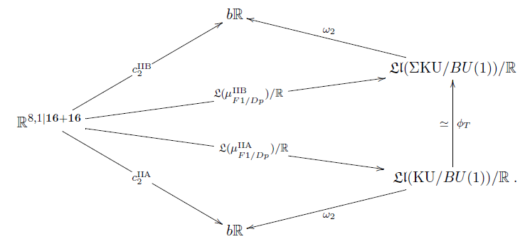
In particular this means that

1. $(\pi^{IIA/IIB}_9)_\ast \left( \mu^{IIA/IIB}_{F1} \right) = - c_2^{IIA/IIB}$.

2. $(\pi_9^{IIA})_\ast - e_9^{IIA} \wedge (-)\vert_{8+1} \;\colon\; C^{IIA} \mapsto C^{IIB}$.

$\,$

The first of these two conditions is

the super $L_\infty$-version of the axiom for

topological T-duality due to Bouwknegt-Evslin-Mathai 04.

$\,$

$\,$

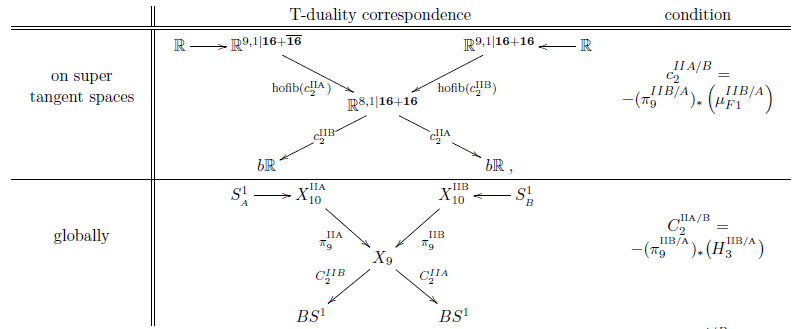
To understand the second condition

pass to the correspondence super $L_\infty$-algebra.

$\,$

Proposition

(Fiorenza-Sati-Schreiber 16b, prop. 6.2)

We have a diagram of super $L_\infty$-algebras of the following form

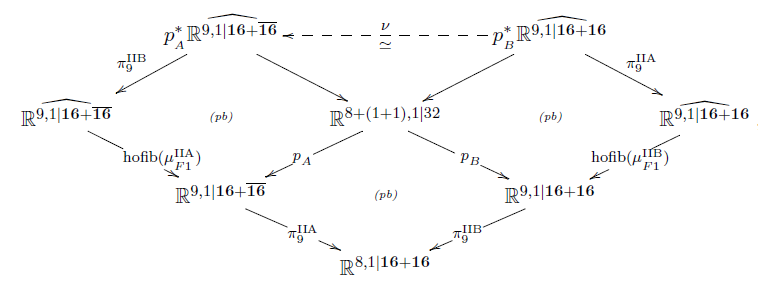
such that on the classifying 3-cocycles

$\nu$ is given by the Poincaré form

$$\mathcal{P} := e_9^{\mathrm{IIA}} \wedge e_9^{\mathrm{IIB}}$$

as

$$p_B^\ast (\mu_{{}_{F1}}^{\mathrm{IIB}} )- p_A^\ast (\mu_{{}_{F1}}^{\mathrm{IIA}}) = d \mathcal{P} \,.$$

$\,$

This now is the super $L_\infty$-version of the

refined formulation of topological T-duality

due to Bunke-Schick 04:

$\,$

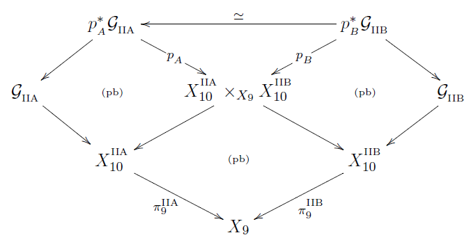
Proposition

(Fiorenza-Sati-Schreiber 16b, prop. 64)

The integral transform of pull-push through this correspondence is an isomorphism

$$(\pi_9^{\mathrm{IIA}})_\ast \circ \nu^\ast \circ (\pi_9^{\mathrm{IIB}})^\ast \;:\; H_{\mu_{F1}^{\mathrm{IIA}}} \left( \mathbb{R}^{9,1\vert \mathbf{16} + \overline{\mathbf{16}}}, \mathfrak{l}(\mathrm{KU}) \right) \longrightarrow H_{\mu_{F1}^{\mathrm{IIB}}} \left( \mathbb{R}^{9,1\vert \mathbf{16} + {\mathbf{16}}}, \mathfrak{l}(\Sigma \mathrm{KU}) \right)$$

Moreover, it identifies the type IIA D-brane cocycles with those of type IIB (from def. ), as in Theorem :

$$\begin{aligned} \exp(-f_2^{\mathrm{IIB}}) \wedge C^{\mathrm{IIB}} & = (\pi_9^{\mathrm{IIA}})_\ast \circ \nu^\ast \circ (\pi_9^{\mathrm{IIB}})^\ast \left( \exp(-f_2^{\mathrm{IIA}}) \wedge C^{\mathrm{IIA}} \right) \\ & = (\pi_9^{\mathrm{IIA}})_\ast \left( \exp(\mathcal{P}) \wedge (\pi_9^{\mathrm{IIB}})^\ast \left( \exp(-f^{\mathrm{IIA}}_2) \wedge C^{\mathrm{IIA}} \right) \right) \end{aligned} \,,$$

Proof

One checks that

$$(\pi_9^{\mathrm{IIA}})_\ast \left( \exp(\mathcal{P}) \wedge (\pi_9^{\mathrm{IIB}})^\ast \left( - \right) \right) = (\pi_9^{\mathrm{IIA}})_\ast(-) - e_9^{IIA} \wedge (- )\vert|_{8+1} \,.$$

With this the statement follows from theorem , item 2.

$\,$

$\,$

Prop. is the super $L_\infty$-algebraic analog of the Bunke-Schick 04, theorem 3.13.

In fact on CE-algebras this is the Buscher rules for RR-fields

also known as Hori’s formula (Hori 99).

$\,$

To see why the above correspondence as in Bunke-Schick 04

follows from the double dimensional reduction isomorphism $\phi_T$

it is useful to break up the doubly dimensionally reduced cocycles $\mathcal{L}( \, \mu_{F1,Dp}^{IIA/B} \, )$

into the part for the fiber bundle and the part for the K-cocycles:

$\,$

Definition

The delooped T-duality Lie 2-algebra $B \mathcal{T}_1$

is the homotopy fiber of the cup square of the first Chern class

$$B \mathcal{T}_1 \overset{}{\longrightarrow} B \mathbb{R} \oplus B \mathbb{R} \overset{\phantom{A}c_1 \cup \tilde c_1 \phantom{A}}{\longrightarrow} B^3 \mathbb{R}$$

hence by prop.

$$CE( B \mathcal{T}_1 ) \;=\; \left\{ \array{ d c_2 = 0, \;\; d \tilde c_2 = 0 \\ d h_3 = - c_2 \wedge \tilde c_2 } \right\} \,.$$

$\,$

Proposition

(FSS 16b, prop. 7.3)

The dimensionally reduced twistd K-theory coefficients from prop.

sit in a homotopy fiber sequence of the form

$$\array{ \mathfrak{l}(\, KU \oplus \Sigma KU \,) &\longrightarrow& \mathfrak{l}(\, \mathcal{L}( KU/BU(1))/S 1 \,) \\ && \downarrow \\ && B \mathcal{T}_1 }$$

exhibiting (via NSS 12) an ∞-action

of the T-duality Lie 2-algebra from def.

on $\mathfrak{l}(\, KU \oplus \Sigma KU \,)$.

$\,$

Proposition

(FSS 16b, prop. 7.5)

The homotopy fiber of the cyclified IIA/B cocycles (theorem )

projected to the T-duality Lie 2-algebra $B \mathcal{T}_1$ (def. )

are the super $L_\infty$-algeberas $p_{A}^\ast \widehat{ \mathbb{R}^{9,1 \vert \mathbf{16} + \overline{\mathbf{16}}} }$ and $p_B^\ast( \widehat{ \mathbb{R}^{9,1\vert \mathbf{16} + \mathbf{16}} } )$ from prop.

hence the Bunke-Schick 04-type correspondence

follows from theorem

via $\infty$-functoriality of homotopy fibers:

$\,$

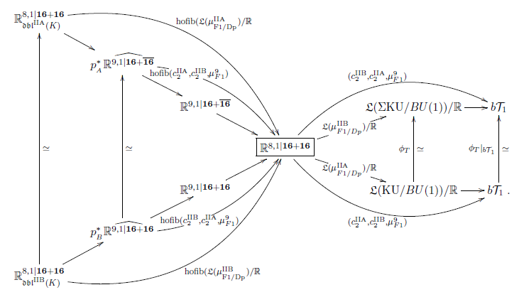
Prop. implies that we may study T-duality

in terms of principal 2-bundles for the T-duality 2-group

over 9d super-manifolds locally modeled on $\mathbb{R}^{8,1\vert \mathbf{16} + \mathbf{16}}$.

This is the supergeometric refinement

of the 2-bundle perspective on T-folds due to (Nikolaus 14).

$\,$

IIB/F

(…)

FSS16b, section 7

(…)

$\,$

$\,$

References

The interpretation of Fierz identities as relations satisfied by Clebsch-Gordan coefficients in the representation ring of the spin group originates in

• Riccardo D'Auria, Pietro Fré, E. Maina, Tullio Regge A New Group Theoretical Technique for the Analysis of Bianchi Identities and Its Application to the Auxiliary Field Problem of $D=5$ Supergravity, Annals Phys. 139 (1982) 93 (doi:10.1016/0003-4916(82)90007-090007-0), spire)

where it was applied to $Spin(4,1)$, relevant in 5-dimensional supergravity.

By this method the Fierz identities for $Spin(9,1)$ (relevant in heterotic supergravity and type II supergravity) are discussed in

• Riccardo D'Auria, Pietro Fré, Geometric Structure of $N=1, D=10$ and $N=4, D=4$ Super Yang-Mills Theory, Nucl. Phys. B196 (1982) 205 (spire)

see also appendix C of

• José Figueroa-O'Farrill, Emily Hackett-Jones, George Moutsopoulos, The Killing superalgebra of ten-dimensional supergravity backgrounds, Class.Quant.Grav.24:3291-3308,2007 (arXiv:hep-th/0703192)

and the Fierz identities for $Spin(10,1)$ (relevant in 11-dimensional supergravity) were tabulated in

• Riccardo D'Auria, Pietro Fré, pages 12, 13 of Geometric Supergravity in D=11 and its hidden supergroup, Nuclear Physics B201 (1982) (errata)

see also

• S. Naito, K. Osada, T. Fukui, Fierz Identities and Invariance of Eleven-dimensional Supergravity Action, Phys.Rev. D34 (1986) 536-552 (spire)

A textbook account of the representation ring method and summary of these results is in

• Leonardo Castellani, Riccardo D'Auria, Pietro Fré, chapter II.8 of Supergravity and Superstrings - A Geometric Perspective, World Scientific (1991)

See also

• C. C. Nishi, Simple derivation of general Fierz-type identities, Am. J. Phys. 73 (2005) 1160-1163 (arXiv:hep-ph/0412245)

From the point of view of division algebras and supersymmetry the Fierz identities that give the vanishing of trilinear and of quadratic terms in spinors in certain dimensions are discussed in

• John Huerta, section 2.4 Division Algebras, Supersymmetry and Higher Gauge Theory (arXiv:1106.3385)

The recognition of some Fierz identities as cocycle conditions defining the higher WZW terms of the super p-branes is due to

• Marc Henneaux, Luca Mezincescu, A Sigma Model Interpretation of Green-Schwarz Covariant Superstring Action, Phys.Lett. B152 (1985) 340 (web)

• Eric Bergshoeff, Ergin Sezgin, Paul Townsend, Supermembranes and eleven dimensional supergravity, Phys.Lett. B189 (1987) 75-78, In Mike Duff, (ed.), The World in Eleven Dimensions 69-72 (pdf, spire)

• Anna Achúcarro, Jonathan Evans, Paul Townsend, David Wiltshire, Super $p$-Branes, Phys. Lett. B 198 (1987) 441 (spire, pdf)

• Igor Bandos, Kurt Lechner, Alexei Nurmagambetov, Paolo Pasti, Dmitri Sorokin, Mario Tonin, Covariant Action for the Super-Five-Brane of M-Theory, Phys. Rev. Lett. 78 (1997) 4332-4334 (arXiv:hep-th/9701149)

The identification of the worldvolume conformal field theories on solitonic branes (black branes) as the perturbation theory of fundamenal super p-branes about asymptotic singular loci in BPS state supergravity solutions is due to

• Piet Claus, Renata Kallosh, Antoine Van Proeyen, M 5-brane and superconformal $(0,2)$ tensor multiplet in 6 dimensions, Nucl.Phys. B518 (1998) 117-150 (arXiv:hep-th/9711161)

• Piet Claus, Renata Kallosh, J. Kumar, Paul Townsend, Antoine Van Proeyen, Conformal Theory of M2, D3, M5 and ‘D1+D5’ Branes, JHEP 9806 (1998) 004 (arXiv:hep-th/9801206)

• Gianguido Dall’Agata, Davide Fabbri, Christophe Fraser, Pietro Fré, Piet Termonia, Mario Trigiante, The $Osp(8|4)$ singleton action from the supermembrane, Nucl.Phys.B542:157-194, 1999 (arXiv:hep-th/9807115)

• Paolo Pasti, Dmitri Sorokin, Mario Tonin, Branes in Super-AdS Backgrounds and Superconformal Theories, Talk given by D.S. at the International Workshop “persymmetry and Quantum Symmetries’’, JINR, Dubna, Russia, July 26-31, 1999 (arXiv:hep-th/9912076)

The bosonic string Lie 2-algebra is discussed in the appendix of

• John Baez, Alissa Crans, Urs Schreiber, Danny Stevenson, From loop groups to 2-groups, Homology Homotopy Appl. Volume 9, Number 2 (2007), 101-135. (arXiv:math/0504123)

Its role in Green-Schwarz anomaly cancellation is discussed in

• Hisham Sati, Urs Schreiber, Jim Stasheff, Twisted Differential String and Fivebrane Structures, Communications in Mathematical Physics, Volume 315, Issue 1 (2012) (arXiv:0910.4001)

and its role in the flux quantization of the supergravity C-field in

• Domenico Fiorenza, Hisham Sati, Urs Schreiber, The moduli 3-stack of the C-field, Communications in Mathematical Physics, Volume 333, Issue 1 (2015), Page 117-151 (arXiv:1202.2455)

and

• Domenico Fiorenza, Hisham Sati, Urs Schreiber, Multiple M5-branes, String 2-connections, and 7d nonabelian Chern-Simons theory, Advances in Theoretical and Mathematical Physics, Volume 18, Number 2 (2014) (arXiv:1201.5277)

Our discussion of L-infinity algebra cohomology is due to

• Hisham Sati, Urs Schreiber, Jim Stasheff, L-infinity algebra connections and applications to String- and Chern-Simons n-transport, in Quantum Field Theory, Birkhäuser (2009) 303-424 (arXiv:0801.3480)

The observation of the brane bouquet in super $L_\infty$-algebra and the general construction of higher WZW terms from higher $L_\infty$-cocycles is due to

• Domenico Fiorenza, Hisham Sati, Urs Schreiber, Super Lie n-algebra extensions, higher WZW models and super p-branes with tensor multiplet fields International Journal of Geometric Methods in Modern Physics Volume 12, Issue 02 (2015) 1550018, (arXiv:1308.5264)

see also

• John Huerta, Hisham Sati, Urs Schreiber, Real ADE-equivariant (co)homotopy and Super M-branes, Comm .in Math. Phys. 371 (2019) 425 [doi:10.1007/s00220-019-03442-3, arXiv:1805.05987]

The homotopy-descent of the M5-brane cocycle and of the type IIA D-brane cocycles is due to

• Domenico Fiorenza, Hisham Sati, Urs Schreiber, The WZW term of the M5-brane and differential cohomotopy, J. Math. Phys. 56, 102301 (2015) (arXiv:1506.07557)

• Domenico Fiorenza, Hisham Sati, Urs Schreiber, Rational sphere valued supercocycles in M-theory, Journal of Geometry and Physics, Volume 114 (2017) (arXiv:1606.03206)

The derivation of supersymmetric topological T-duality, rationally, and of the higher super Cartan geometry for super T-folds is due to

• Domenico Fiorenza, Hisham Sati, Urs Schreiber, T-Duality from super Lie n-algebra cocycles for super p-branes, ATMP 22 5 (2018) (arXiv:1611.06536, doi:10.4310/ATMP.2018.v22.n5.a3)

and the mathematical formulation of double dimensional reduction that this uses is further discussed in

• Vincent Braunack-Mayer, Hisham Sati, Urs Schreiber, Section 2.2 of: Gauge enhancement of Super M-Branes via rational parameterized stable homotopy theory, Communications in Mathematical Physics 371: 197 (2019) (arXiv:1806.01115, doi:10.1007/s00220-019-03441-4)

The derivation of the process of higher invariant extensions that leads from the superpoint to 11-dimensional supergravity:

• John Huerta, Urs Schreiber, M-Theory from the Superpoint, Letters in Mathematical Physics 108 (2018) 2695–2727 (arXiv:1702.01774, doi:10.1007/s11005-018-1110-z)

General discussion of twisted cohomology is in:

• Thomas Nikolaus, Urs Schreiber, Danny Stevenson, Principal ∞-bundles – General theory, Journal of Homotopy and Related Structures, Volume 10, Issue 4 (2015) (arXiv:1207.0248)

• Domenico Fiorenza, Hisham Sati, Urs Schreiber, The Character Map in Twisted Non-Abelian Cohomology (arXiv:2009.11909)

Foundations and parts of the story is in:

• Urs Schreiber, differential cohomology in a cohesive topos, Thesis