nLab geometry of physics -- homotopy types
Basic notions of homotopy theory
Traditionally, mathematics and physics have been founded on set theory, whose concept of sets is that of “bags of distinguishable points”.
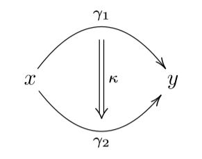
But fundamental physics is governed by the gauge principle. This says that given any two “things”, such as two field histories and , it is in general wrong to ask whether they are equal or not, instead one has to ask where there is a gauge transformation
between them. In mathematics this is called a homotopy.
This principle applies also to gauge transformations/homotopies themselves, and thus leads to gauge-of-gauge transformations or homotopies of homotopies
and so on to ever higher gauge transformations or higher homotopies:
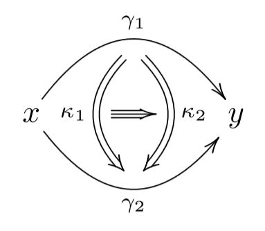
This shows that what an here are elements of is not really a set in the sense of set theory. Instead, such a collection of elements with higher gauge transformations/higher homotopies between them is called a homotopy type.
Hence the theory of homotopy types – homotopy theory – is much like set theory, but with the concept of gauge transformation/homotopy built right into its foundations. Homotopy theory is gauged mathematics.
A classical model for homotopy types are simply topological spaces: Their points represent the elements, the continuous paths between points represent the gauge transformations, and continuous deformations of paths represent higher gauge transformations. A central result of homotopy theory is the proof of the homotopy hypothesis, which says that under this identification homotopy types are equivalent to topological spaces viewed, in turn, up to “weak homotopy equivalence”.
In the special case of a homotopy type with a single element , the gauge transformations necessarily go from to itself and hence form a group of symmetries of .
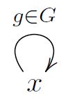
This way homotopy theory subsumes group theory.
If there are higher order gauge-of-gauge transformations/homotopies of homotopies between these symmetry group-elements, then one speaks of 2-groups, 3-groups, … n-groups, and eventually of ∞-groups. When homotopy types are represented by topological spaces, then ∞-groups are represented by topological groups.
This way homotopy theory subsumes parts of topological group theory.
Since, generally, there is more than one element in a homotopy type, these are like “groups with several elements”, and as such they are called groupoids (Def. ).
If there are higher order gauge-of-gauge transformations/homotopies of homotopies between the transformations in such a groupoid, one speaks of 2-groupoids, 3-groupoids, … n-groupoids, and eventually of ∞-groupoids. The plain sets are recovered as the special case of 0-groupoids.
Due to the higher orders appearing here, mathematical structures based not on sets but on homotopy types are also called higher structures.
Hence homotopy types are equivalently ∞-groupoids. This perspective makes explicit that homotopy types are the unification of plain sets with the concept of gauge-symmetry groups.
An efficient way of handling ∞-groupoids is in their explicit guise as Kan complexes (Def. below); these are the non-abelian generalization of the chain complexes used in homological algebra. Indeed, chain homotopy is a special case of the general concept of homotopy, and hence homological algebra forms but a special abelian corner within homotopy theory. Conversely, homotopy theory may be understood as the non-abelian generalization of homological algebra.
Hence, in a self-reflective manner, there are many different but equivalent incarnations of homotopy theory. Below we discuss in turn:
-
∞-groupoids modeled by topological spaces. This is the classical model of homotopy theory familiar from traditional point-set topology, such as covering space-theory.
-
∞-groupoids modeled on simplicial sets, whose fibrant objects are the Kan complexes. This simplicial homotopy theory is Quillen equivalent to topological homotopy theory (the “homotopy hypothesis”), which makes explicit that homotopy theory is not really about topological spaces, but about the ∞-groupoids that these represent.
Ideally, abstract homotopy theory would simply be a complete replacement of set theory, obtained by removing the assumption of strict equality, relaxing it to gauge equivalence/homotopy. As such, abstract homotopy theory would be part and parcel of the foundations of mathematics themselves, not requiring any further discussion. This ideal perspective is the promise of homotopy type theory and may become full practical reality in the next decades.
Until then, abstract homotopy theory has to be formulated on top of the traditional foundations of mathematics provided by set theory, much like one may have to run a Linux emulator on a Windows machine, if one does happen to be stuck with the latter.
A very convenient and powerful such emulator for homotopy theory within set theory is model category theory, originally due to Quillen 67 and highly developed since. This we introduce here.
The idea is to consider ordinary categories (Def. ) but with the understanding that some of their morphisms
should be homotopy equivalences (Def. ), namely similar to isomorphisms (Def. ), but not necessarily satisfying the two equations defining an actual isomorphism
but intended to satisfy this only with equality relaxed to gauge transformation/homotopy:
Such would-be homotopy equivalences are called weak equivalences (Def. below).
In principle, this information already defines a homotopy theory by a construction called simplicial localization, which turns weak equivalences into actual homotopy equivalences in a suitable way.
However, without further tools this construction is unwieldy. The extra structure of a model category (Def. below) on top of a category with weak equivalences provides a set of tools.
The idea here is to abstract (in Def. below) from the evident concepts in topological homotopy theory of left homotopy (Def. ) and right homotopy (Def. ) between continuous functions: These are provided by continuous functions out of a cylinder space or into a path space , respectively, where in both cases the interval space serves to parameterize the relevant gauge transformation/homotopy.
Now a little reflection shows (this was the seminal insight of Quillen 67) that what really matters in this construction of homotopies is that the path space factors the diagonal morphism from a space to its Cartesian product as
while the cylinder serves to factor the codiagonal morphism as
where in both cases “fibration” means something like well behaved surjection, while “cofibration” means something like satisfying the lifting property (Def. below) against fibrations that are also weak equivalences.
Such factorizations subject to lifting properties is what the definition of model category axiomatizes, in some generality. That this indeed provides a good toolbox for handling homotopy equivalences is shown by the Whitehead theorem in model categories (Lemma below), which exhibits all weak equivalences as actual homotopy equivalences after passage to “good representatives” of objects (fibrant/cofibrant resolutions, Def. below). Accordingly, the first theorem of model category theory (Quillen 67, I.1 theorem 1, reproduced as Theorem below), provides a tractable expression for the hom-sets modulo homotopy equivalence of the underlying category with weak equivalences in terms of actual morphisms out of cofibrant resolutions into fibrant resolutions (Lemma below).
This is then generally how model category-theory serves as a model for homotopy theory: All homotopy-theoretic constructions, such as that of long homotopy fiber sequences (Prop. below), are reflected via constructions of ordinary category theory but applied to suitably resolved objects.
Literature (Dwyer-Spalinski 95)
Definition
A model category is
such that
-
the class makes into a category with weak equivalences, def. ;
-
The pairs and are both weak factorization systems, def. .
One says:
-
elements in are weak equivalences,
-
elements in are cofibrations,
-
elements in are fibrations,
-
elements in are acyclic cofibrations,
-
elements in are acyclic fibrations.
The form of def. is due to (Joyal, def. E.1.2). It implies various other conditions that (Quillen 67) demands explicitly, see prop. and prop. below.
We now dicuss the concept of weak factorization systems (Def. below) appearing in def. .
Factorization systems
Definition
Let be any category. Given a diagram in of the form
then an extension of the morphism along the morphism is a completion to a commuting diagram of the form
Dually, given a diagram of the form
then a lift of through is a completion to a commuting diagram of the form
Combining these cases: given a commuting square
then a lifting in the diagram is a completion to a commuting diagram of the form
Given a sub-class of morphisms , then
- a morphism as above is said to have the right lifting property against or to be a -injective morphism if in all square diagrams with on the right and any on the left a lift exists.
dually:
- a morphism is said to have the left lifting property against or to be a -projective morphism if in all square diagrams with on the left and any on the left a lift exists.
Definition
A weak factorization system (WFS) on a category is a pair of classes of morphisms of such that
-
Every morphism of may be factored as the composition of a morphism in followed by one in
-
The classes are closed under having the lifting property, def. , against each other:
-
is precisely the class of morphisms having the left lifting property against every morphisms in ;
-
is precisely the class of morphisms having the right lifting property against every morphisms in .
-
Definition
For a category, a functorial factorization of the morphisms in is a functor
which is a section of the composition functor .
Remark
In def. we are using the following standard notation, see at simplex category and at nerve of a category:
Write and for the ordinal numbers, regarded as posets and hence as categories. The arrow category is equivalently the functor category , while has as objects pairs of composable morphisms in . There are three injective functors , where omits the index in its image. By precomposition, this induces functors . Here
-
sends a pair of composable morphisms to their composition;
-
sends a pair of composable morphisms to the first morphisms;
-
sends a pair of composable morphisms to the second morphisms.
Definition
A weak factorization system, def. , is called a functorial weak factorization system if the factorization of morphisms may be chosen to be a functorial factorization , def. , i.e. such that lands in and in .
Remark
Not all weak factorization systems are functorial, def. , although most (including those produced by the small object argument (prop. below), with due care) are.
Proposition
Let be a category and let be a class of morphisms. Write and , respectively, for the sub-classes of -projective morphisms and of -injective morphisms, def. . Then:
-
Both classes contain the class of isomorphism of .
-
Both classes are closed under composition in .
is also closed under transfinite composition.
-
Both classes are closed under forming retracts in the arrow category (see remark ).
-
is closed under forming pushouts of morphisms in (“cobase change”).
is closed under forming pullback of morphisms in (“base change”).
-
is closed under forming coproducts in .
is closed under forming products in .
Proof
We go through each item in turn.
containing isomorphisms
Given a commuting square
with the left morphism an isomorphism, then a lift is given by using the inverse of this isomorphism . Hence in particular there is a lift when and so . The other case is formally dual.
closure under composition
Given a commuting square of the form
consider its pasting decomposition as
Now the bottom commuting square has a lift, by assumption. This yields another pasting decomposition
and now the top commuting square has a lift by assumption. This is now equivalently a lift in the total diagram, showing that has the right lifting property against and is hence in . The case of composing two morphisms in is formally dual. From this the closure of under transfinite composition follows since the latter is given by colimits of sequential composition and successive lifts against the underlying sequence as above constitutes a cocone, whence the extension of the lift to the colimit follows by its universal property.
closure under retracts
Let be the retract of an , i.e. let there be a commuting diagram of the form.
Then for
a commuting square, it is equivalent to its pasting composite with that retract diagram
Here the pasting composite of the two squares on the right has a lift, by assumption:
By composition, this is also a lift in the total outer rectangle, hence in the original square. Hence has the left lifting property against all and hence is in . The other case is formally dual.
closure under pushout and pullback
Let and and let
be a pullback diagram in . We need to show that has the right lifting property with respect to all . So let
be a commuting square. We need to construct a diagonal lift of that square. To that end, first consider the pasting composite with the pullback square from above to obtain the commuting diagram
By the right lifting property of , there is a diagonal lift of the total outer diagram
By the universal property of the pullback this gives rise to the lift in
In order for to qualify as the intended lift of the total diagram, it remains to show that
commutes. To do so we notice that we obtain two cones with tip :
-
one is given by the morphisms
with universal morphism into the pullback being
-
the other by
- .
with universal morphism into the pullback being
- .
The commutativity of the diagrams that we have established so far shows that the first and second morphisms here equal each other, respectively. By the fact that the universal morphism into a pullback diagram is unique this implies the required identity of morphisms.
The other case is formally dual.
closure under (co-)products
Let be a set of elements of . Since colimits in the presheaf category are computed componentwise, their coproduct in this arrow category is the universal morphism out of the coproduct of objects induced via its universal property by the set of morphisms :
Now let
be a commuting square. This is in particular a cocone under the coproduct of objects, hence by the universal property of the coproduct, this is equivalent to a set of commuting diagrams
By assumption, each of these has a lift . The collection of these lifts
is now itself a compatible cocone, and so once more by the universal property of the coproduct, this is equivalent to a lift in the original square
This shows that the coproduct of the has the left lifting property against all and is hence in . The other case is formally dual.
An immediate consequence of prop. is this:
Corollary
Let be a category with all small colimits, and let be a sub-class of its morphisms. Then every -injective morphism, def. , has the right lifting property, def. , against all -relative cell complexes, def. and their retracts, remark .
Remark
By a retract of a morphism in some category we mean a retract of as an object in the arrow category , hence a morphism such that in there is a factorization of the identity on through
This means equivalently that in there is a commuting diagram of the form
Lemma
In every category the class of isomorphisms is preserved under retracts in the sense of remark .
Proof
For
a retract diagram and an isomorphism, the inverse to is given by the composite
More generally:
Proposition
Given a model category in the sense of def. , then its class of weak equivalences is closed under forming retracts (in the arrow category, see remark ).
Proof
Let
be a commuting diagram in the given model category, with a weak equivalence. We need to show that then also .
First consider the case that .
In this case, factor as a cofibration followed by an acyclic fibration. Since and by two-out-of-three (def. ) this is even a factorization through an acyclic cofibration followed by an acyclic fibration. Hence we obtain a commuting diagram of the following form:
where is uniquely defined and where is any lift of the top middle vertical acyclic cofibration against . This now exhibits as a retract of an acyclic fibration. These are closed under retract by prop. .
Now consider the general case. Factor as an acyclic cofibration followed by a fibration and form the pushout in the top left square of the following diagram
where the other three squares are induced by the universal property of the pushout, as is the identification of the middle horizontal composite as the identity on . Since acyclic cofibrations are closed under forming pushouts by prop. , the top middle vertical morphism is now an acyclic fibration, and hence by assumption and by two-out-of-three so is the middle bottom vertical morphism.
Thus the previous case now gives that the bottom left vertical morphism is a weak equivalence, and hence the total left vertical composite is.
Lemma
Consider a composite morphism
-
If has the left lifting property against , then is a retract of .
-
If has the right lifting property against , then is a retract of .
Proof
We discuss the first statement, the second is formally dual.
Write the factorization of as a commuting square of the form
By the assumed lifting property of against there exists a diagonal filler making a commuting diagram of the form
By rearranging this diagram a little, it is equivalent to
Completing this to the right, this yields a diagram exhibiting the required retract according to remark :
Small object argument
Given a set of morphisms in some category , a natural question is how to factor any given morphism through a relative -cell complex, def. , followed by a -injective morphism, def.
A first approximation to such a factorization turns out to be given simply by forming by attaching all possible -cells to . Namely let
be the set of all ways to find a -cell attachment in , and consider the pushout of the coproduct of morphisms in over all these:
This gets already close to producing the intended factorization:
First of all the resulting map is a -relative cell complex, by construction.
Second, by the fact that the coproduct is over all commuting squres to , the morphism itself makes a commuting diagram
and hence the universal property of the colimit means that is indeed factored through that -cell complex ; we may suggestively arrange that factorizing diagram like so:
This shows that, finally, the colimiting co-cone map – the one that now appears diagonally – almost exhibits the desired right lifting of against the . The failure of that to hold on the nose is only the fact that a horizontal map in the middle of the above diagram is missing: the diagonal map obtained above lifts not all commuting diagrams of into , but only those where the top morphism factors through .
The idea of the small object argument now is to fix this only remaining problem by iterating the construction: next factor in the same way into
and so forth. Since relative -cell complexes are closed under composition, at stage the resulting is still a -cell complex, getting bigger and bigger. But accordingly, the failure of the accompanying to be a -injective morphism becomes smaller and smaller, for it now lifts against all diagrams where factors through , which intuitively is less and less of a condition as the grow larger and larger.
The concept of small object is just what makes this intuition precise and finishes the small object argument. For the present purpose we just need the following simple version:
Definition
For a category and a sub-set of its morphisms, say that these have small domains if there is an ordinal (def. ) such that for every and for every -relative cell complex given by a transfinite composition (def. )
every morphism factors through a stage of order :
The above discussion proves the following:
Proposition
(small object argument)
Let be a locally small category with all small colimits. If a set of morphisms has all small domains in the sense of def. , then every morphism in factors through a -relative cell complex, def. , followed by a -injective morphism, def.
Homotopy
We discuss how the concept of homotopy is abstractly realized in model categories, def. .
Definition
Let be a model category, def. , and an object.
- A path space object for is a factorization of the diagonal as
where is a weak equivalence and is a fibration.
- A cylinder object for is a factorization of the codiagonal (or “fold map”) as
where is a weak equivalence. and is a cofibration.
Remark
For every object in a model category, a cylinder object and a path space object according to def. exist: the factorization axioms guarantee that there exists
-
a factorization of the codiagonal as
-
a factorization of the diagonal as
The cylinder and path space objects obtained this way are actually better than required by def. : in addition to being just a weak equivalence, for these this is actually an acyclic fibration, and dually in addition to being a weak equivalence, for these it is actually an acyclic cofibrations.
Some authors call cylinder/path-space objects with this extra property “very good” cylinder/path-space objects, respectively.
One may also consider dropping a condition in def. : what mainly matters is the weak equivalence, hence some authors take cylinder/path-space objects to be defined as in def. but without the condition that is a cofibration and without the condition that is a fibration. Such authors would then refer to the concept in def. as “good” cylinder/path-space objects.
The terminology in def. follows the original (Quillen 67, I.1 def. 4). With the induced concept of left/right homotopy below in def. , this admits a quick derivation of the key facts in the following, as we spell out below.
Lemma
Let be a model category. If is cofibrant, then for every cylinder object of , def. , not only is a cofibration, but each
is an acyclic cofibration separately.
Dually, if is fibrant, then for every path space object of , def. , not only is a cofibration, but each
is an acyclic fibration separately.
Proof
We discuss the case of the path space object. The other case is formally dual.
First, that the component maps are weak equivalences follows generally: by definition they have a right inverse and so this follows by two-out-of-three (def. ).
But if is fibrant, then also the two projection maps out of the product are fibrations, because they are both pullbacks of the fibration
hence is the composite of two fibrations, and hence itself a fibration, by prop. .
Path space objects are very non-unique as objects up to isomorphism:
Example
If is a fibrant object in a model category, def. , and for and two path space objects for , def. , then the fiber product is another path space object for : the pullback square
gives that the induced projection is again a fibration. Moreover, using lemma and two-out-of-three (def. ) gives that is a weak equivalence.
For the case of the canonical topological path space objects of def , with then this new path space object is , the mapping space out of the standard interval of length 2 instead of length 1.
Definition
(abstract left homotopy and abstract right homotopy
Let be two parallel morphisms in a model category.
- A left homotopy is a morphism from a cylinder object of , def. , such that it makes this diagram commute:
- A right homotopy is a morphism to some path space object of , def. , such that this diagram commutes:
Lemma
Let be two parallel morphisms in a model category.
-
Let be cofibrant. If there is a left homotopy then there is also a right homotopy (def. ) with respect to any chosen path space object.
-
Let be fibrant. If there is a right homotopy then there is also a left homotopy with respect to any chosen cylinder object.
In particular if is cofibrant and is fibrant, then by going back and forth it follows that every left homotopy is exhibited by every cylinder object, and every right homotopy is exhibited by every path space object.
Proof
We discuss the first case, the second is formally dual. Let be the given left homotopy. Lemma implies that we have a lift in the following commuting diagram
where on the right we have the chosen path space object. Now the composite is a right homotopy as required:
Proposition
For a cofibrant object in a model category and a fibrant object, then the relations of left homotopy and of right homotopy (def. ) on the hom set coincide and are both equivalence relations.
Proof
That both relations coincide under the (co-)fibrancy assumption follows directly from lemma .
The symmetry and reflexivity of the relation is obvious.
That right homotopy (hence also left homotopy) with domain is a transitive relation follows from using example to compose path space objects.
The homotopy category
We discuss the construction that takes a model category, def. , and then universally forces all its weak equivalences into actual isomorphisms.
Definition
(homotopy category of a model category)
Let be a model category, def. . Write for the category whose
-
objects are those objects of which are both fibrant and cofibrant;
-
morphisms are the homotopy classes of morphisms of , hence the equivalence classes of morphism under the equivalence relation of prop. ;
and whose composition operation is given on representatives by composition in .
This is, up to equivalence of categories, the homotopy category of the model category .
Proposition
Def. is well defined, in that composition of morphisms between fibrant-cofibrant objects in indeed passes to homotopy classes.
Proof
Fix any morphism between fibrant-cofibrant objects. Then for precomposition
to be well defined, we need that with also . But by prop we may take the homotopy to be exhibited by a right homotopy , for which case the statement is evident from this diagram:
For postcomposition we may choose to exhibit homotopy by left homotopy and argue dually.
We now spell out that def. indeed satisfies the universal property that defines the localization of a category with weak equivalences at its weak equivalences.
Lemma
(Whitehead theorem in model categories)
Let be a model category. A weak equivalence between two objects which are both fibrant and cofibrant is a homotopy equivalence (1).
Proof
By the factorization axioms in the model category and by two-out-of-three (def. ), every weak equivalence factors through an object as an acyclic cofibration followed by an acyclic fibration. In particular it follows that with and both fibrant and cofibrant, so is , and hence it is sufficient to prove that acyclic (co-)fibrations between such objects are homotopy equivalences.
So let be an acyclic fibration between fibrant-cofibrant objects, the case of acyclic cofibrations is formally dual. Then in fact it has a genuine right inverse given by a lift in the diagram
To see that is also a left inverse up to left homotopy, let be any cylinder object on (def. ), hence a factorization of the codiagonal on as a cofibration followed by a an acyclic fibration
and consider the commuting square
which commutes due to being a genuine right inverse of . By construction, this commuting square now admits a lift , and that constitutes a left homotopy .
Definition
(fibrant resolution and cofibrant resolution)
Given a model category , consider a choice for each object of
-
a factorization
of the initial morphism (Def. ), such that when is already cofibrant then ;
-
a factorization
of the terminal morphism (Def. ), such that when is already fibrant then .
Write then
for the functor to the homotopy category, def. , which sends an object to the object and sends a morphism to the homotopy class of the result of first lifting in
and then lifting (here: extending) in
Proof
First of all, the object is indeed both fibrant and cofibrant (as well as related by a zig-zag of weak equivalences to ):
Now to see that the image on morphisms is well defined. First observe that any two choices of the first lift in the definition are left homotopic to each other, exhibited by lifting in
Hence also the composites are left homotopic to each other, and since their domain is cofibrant, then by lemma they are also right homotopic by a right homotopy . This implies finally, by lifting in
that also and are right homotopic, hence that indeed represents a well-defined homotopy class.
Finally to see that the assignment is indeed functorial, observe that the commutativity of the lifting diagrams for and imply that also the following diagram commutes
Now from the pasting composite
one sees that is a lift of and hence the same argument as above gives that it is homotopic to the chosen .
For the following, recall the concept of natural isomorphism between functors: for two functors, then a natural transformation is for each object a morphism in , such that for each morphism in the following is a commuting square:
Such is called a natural isomorphism if its are isomorphisms for all objects .
Definition
(localization of a category category with weak equivalences)
For a category with weak equivalences, its localization at the weak equivalences is, if it exists,
such that
-
sends weak equivalences to isomorphisms;
-
is universal with this property, in that:
for any functor out of into any category , such that takes weak equivalences to isomorphisms, it factors through up to a natural isomorphism
and this factorization is unique up to unique isomorphism, in that for and two such factorizations, then there is a unique natural isomorphism making the evident diagram of natural isomorphisms commute.
Theorem
(convenient localization of model categories)
For a model category, the functor in def. (for any choice of and ) exhibits as indeed being the localization of the underlying category with weak equivalences at its weak equivalences, in the sense of def. :
Proof
First, to see that that indeed takes weak equivalences to isomorphisms: By two-out-of-three (def. ) applied to the commuting diagrams shown in the proof of lemma , the morphism is a weak equivalence if is:
With this the “Whitehead theorem for model categories”, lemma , implies that represents an isomorphism in .
Now let be any functor that sends weak equivalences to isomorphisms. We need to show that it factors as
uniquely up to unique natural isomorphism. Now by construction of and in def. , is the identity on the full subcategory of fibrant-cofibrant objects. It follows that if exists at all, it must satisfy for all with and both fibrant and cofibrant that
(hence in particular ).
But by def. that already fixes on all of , up to unique natural isomorphism. Hence it only remains to check that with this definition of there exists any natural isomorphism filling the diagram above.
To that end, apply to the above commuting diagram to obtain
Here now all horizontal morphisms are isomorphisms, by assumption on . It follows that defining makes the required natural isomorphism:
Remark
Due to theorem we may suppress the choices of cofibrant and fibrant replacement in def. and just speak of the localization functor
up to natural isomorphism.
In general, the localization of a category with weak equivalences (def. ) may invert more morphisms than just those in . However, if the category admits the structure of a model category , then its localization precisely only inverts the weak equivalences:
Proposition
(localization of model categories inverts precisely the weak equivalences)
Let be a model category (def. ) and let be its localization functor (def. , theorem ). Then a morphism in is a weak equivalence precisely if is an isomorphism in .
(e.g. Goerss-Jardine 96, II, prop 1.14)
While the construction of the homotopy category in def. combines the restriction to good (fibrant/cofibrant) objects with the passage to homotopy classes of morphisms, it is often useful to consider intermediate stages:
Definition
Given a model category , write
for the system of full subcategory inclusions of:
-
the category of fibrant-cofibrant objects ,
all regarded a categories with weak equivalences (def. ), via the weak equivalences inherited from , which we write , and .
Remark
(categories of fibrant objects and cofibration categories)
Of course the subcategories in def. inherit more structure than just that of categories with weak equivalences from . and each inherit “half” of the factorization axioms. One says that has the structure of a “fibration category” called a “Brown-category of fibrant objects”, while has the structure of a “cofibration category”.
We discuss properties of these categories of (co-)fibrant objects below in Homotopy fiber sequences.
The proof of theorem immediately implies the following:
Corollary
For a model category, the restriction of the localization functor from def. (using remark ) to any of the sub-categories with weak equivalences of def.
exhibits equivalently as the localization also of these subcategories with weak equivalences, at their weak equivalences. In particular there are equivalences of categories
The following says that for computing the hom-sets in the homotopy category, even a mixed variant of the above will do; it is sufficient that the domain is cofibrant and the codomain is fibrant:
Lemma
(hom-sets of homotopy category via mapping cofibrant resolutions into fibrant resolutions)
For with cofibrant and fibrant, and for fibrant/cofibrant replacement functors as in def. , then the morphism
(on homotopy classes of morphisms, well defined by prop. ) is a natural bijection.
Proof
We may factor the morphism in question as the composite
This shows that it is sufficient to see that for cofibrant and fibrant, then
is an isomorphism, and dually that
is an isomorphism. We discuss this for the former; the second is formally dual:
First, that is surjective is the lifting property in
which says that any morphism comes from a morphism under postcomposition with .
Second, that is injective is the lifting property in
which says that if two morphisms become homotopic after postcomposition with , then they were already homotopic before.
We record the following fact which will be used in part 1.1 (here):
Lemma
Let be a model category (def. ). Then every commuting square in its homotopy category (def. ) is, up to isomorphism of squares, in the image of the localization functor of a commuting square in (i.e.: not just commuting up to homotopy).
Proof
Let
be a commuting square in the homotopy category. Writing the same symbols for fibrant-cofibrant objects in and for morphisms in representing these, then this means that in there is a left homotopy of the form
Consider the factorization of the top square here through the mapping cylinder of
This exhibits the composite as an alternative representative of in , and as an alternative representative for , and the commuting square
as an alternative representative of the given commuting square in .
Derived functors
Definition
For and two categories with weak equivalences, def. , then a functor is called a homotopical functor if it sends weak equivalences to weak equivalences.
Definition
Given a homotopical functor (def. ) between categories with weak equivalences whose homotopy categories and exist (def. ), then its (“total”) derived functor is the functor between these homotopy categories which is induced uniquely, up to unique isomorphism, by their universal property (def. ):
Remark
While many functors of interest between model categories are not homotopical in the sense of def. , many become homotopical after restriction to the full subcategories of fibrant objects or of cofibrant objects, def. . By corollary this is just as good for the purpose of homotopy theory.
Therefore one considers the following generalization of def. :
Definition
(left and right derived functors)
Consider a functor out of a model category (def. ) into a category with weak equivalences (def. ).
-
If the restriction of to the full subcategory of fibrant object becomes a homotopical functor (def. ), then the derived functor of that restriction, according to def. , is called the right derived functor of and denoted by :
-
If the restriction of to the full subcategory of cofibrant object becomes a homotopical functor (def. ), then the derived functor of that restriction, according to def. , is called the left derived functor of and denoted by :
The key fact that makes def. practically relevant is the following:
Proposition
Let be a model category with full subcategories of fibrant objects and of cofibrant objects respectively (def. ). Let be a category with weak equivalences.
-
A functor out of the category of fibrant objects
is a homotopical functor, def. , already if it sends acyclic fibrations to weak equivalences.
-
A functor out of the category of cofibrant objects
is a homotopical functor, def. , already if it sends acyclic cofibrations to weak equivalences.
The following proof refers to the factorization lemma, whose full statement and proof we postpone to further below (lemma ).
Proof
We discuss the case of a functor on a category of fibrant objects , def. . The other case is formally dual.
Let be a weak equivalence in . Choose a path space object (def. ) and consider the diagram
where the square is a pullback and on the top left is our notation for the universal cone object. (Below we discuss this in more detail, it is the mapping cocone of , def. ).
Here:
-
is an acyclic fibration because it is the pullback of .
-
is a weak equivalence, because the factorization lemma states that the composite vertical morphism factors through a weak equivalence, hence if is a weak equivalence, then is by two-out-of-three (def. ).
Now apply the functor to this diagram and use the assumption that it sends acyclic fibrations to weak equivalences to obtain
But the factorization lemma , in addition says that the vertical composite is a fibration, hence an acyclic fibration by the above. Therefore also is a weak equivalence. Now the claim that also is a weak equivalence follows with applying two-out-of-three (def. ) twice.
Corollary
Let be model categories and consider a functor. Then:
-
If preserves cofibrant objects and acyclic cofibrations between these, then its left derived functor (def. ) exists, fitting into a diagram
-
If preserves fibrant objects and acyclic fibrants between these, then its right derived functor (def. ) exists, fitting into a diagram
Proposition
(construction of left/right derived functors)
Let be a functor between two model categories (def. ).
-
If preserves fibrant objects and weak equivalences between fibrant objects, then the total right derived functor (def. ) in
is given, up to isomorphism, on any object by appying to a fibrant replacement of and then forming a cofibrant replacement of the result:
-
If preserves cofibrant objects and weak equivalences between cofibrant objects, then the total left derived functor (def. ) in
is given, up to isomorphism, on any object by appying to a cofibrant replacement of and then forming a fibrant replacement of the result:
Proof
We discuss the first case, the second is formally dual. By the proof of theorem we have
But since is a homotopical functor on fibrant objects, the cofibrant replacement morphism is a weak equivalence in , hence becomes an isomorphism under . Therefore
Now since is assumed to preserve fibrant objects, is fibrant in , and hence acts on it (only) by cofibrant replacement.
Quillen adjunctions
In practice it turns out to be useful to arrange for the assumptions in corollary to be satisfied by pairs of adjoint functors (Def. ). Recall that this is a pair of functors and going back and forth between two categories
such that there is a natural bijection between hom-sets with on the left and those with on the right (?):
for all objects and . This being natural (Def. ) means that is a natural transformation, hence that for all morphisms and the following is a commuting square:
We write to indicate such an adjunction and call the left adjoint and the right adjoint of the adjoint pair.
The archetypical example of a pair of adjoint functors is that consisting of forming Cartesian products and forming mapping spaces , as in the category of compactly generated topological spaces of def. .
If is any morphism, then the image is called its adjunct, and conversely. The fact that adjuncts are in bijection is also expressed by the notation
For an object , the adjunct of the identity on is called the adjunction unit .
For an object , the adjunct of the identity on is called the adjunction counit .
Adjunction units and counits turn out to encode the adjuncts of all other morphisms by the formulas
-
.
Definition
Let be model categories. A pair of adjoint functors (Def. ) between them
is called a Quillen adjunction, to be denoted
and , are called left/right Quillen functors, respectively, if the following equivalent conditions are satisfied:
-
preserves cofibrations and preserves fibrations;
-
preserves acyclic cofibrations and preserves acyclic fibrations;
-
preserves cofibrations and acyclic cofibrations;
-
preserves fibrations and acyclic fibrations.
Proof
First observe that
-
(i) A left adjoint between model categories preserves acyclic cofibrations precisely if its right adjoint preserves fibrations.
-
(ii) A left adjoint between model categories preserves cofibrations precisely if its right adjoint preserves acyclic fibrations.
We discuss statement (i), statement (ii) is formally dual. So let be an acyclic cofibration in and a fibration in . Then for every commuting diagram as on the left of the following, its -adjunct is a commuting diagram as on the right here:
If preserves acyclic cofibrations, then the diagram on the right has a lift, and so the -adjunct of that lift is a lift of the left diagram. This shows that has the right lifting property against all acylic cofibrations and hence is a fibration. Conversely, if preserves fibrations, the same argument run from right to left gives that preserves acyclic fibrations.
Now by repeatedly applying (i) and (ii), all four conditions in question are seen to be equivalent.
The following is the analog of adjunction unit and adjunction counit (Def. ):
Definition
Let and be model categories (Def. ), and let
be a Quillen adjunction (Def. ). Then
-
a derived adjunction unit at an object is a composition of the form
where
-
is the ordinary adjunction unit (Def. );
-
is a cofibrant resolution in (Def. );
-
is a fibrant resolution in (Def. );
-
-
a derived adjunction counit at an object is a composition of the form
where
-
is the ordinary adjunction counit (Def. );
-
is a fibrant resolution in (Def. );
-
is a cofibrant resolution in (Def. ).
-
We will see that Quillen adjunctions induce ordinary adjoint pairs of derived functors on homotopy categories (Prop. ). For this we first consider the following technical observation:
Lemma
(right Quillen functors preserve path space objects)
Let be a Quillen adjunction, def. .
-
For a fibrant object and a path space object (def. ), then is a path space object for .
-
For a cofibrant object and a cylinder object (def. ), then is a cylinder object for .
Proof
Consider the second case, the first is formally dual.
First Observe that because is left adjoint and hence preserves colimits, hence in particular coproducts.
Hence
is a cofibration.
Second, with cofibrant then also is a cofibrantion, since is a cofibration (lemma ). Therefore by Ken Brown's lemma (prop. ) preserves the weak equivalence .
Proposition
For a Quillen adjunction, def. , also the corresponding left and right derived functors (Def. , via cor. ) form a pair of adjoint functors
Moreover, the adjunction unit and adjunction counit of this derived adjunction are the images of the derived adjunction unit and derived adjunction counit (Def. ) under the localization functors (Theorem ).
Proof
For the first statement, by def. and lemma it is sufficient to see that for with cofibrant and fibrant, then there is a natural bijection
Since by the adjunction isomorphism for such a natural bijection exists before passing to homotopy classes , it is sufficient to see that this respects homotopy classes. To that end, use from lemma that with a cylinder object for , def. , then is a cylinder object for . This implies that left homotopies
given by
are in bijection to left homotopies
given by
This establishes the adjunction. Now regarding the (co-)units: We show this for the adjunction unit, the case of the adjunction counit is formally dual.
First observe that for , then the defining commuting square for the left derived functor from def.
(using fibrant and fibrant/cofibrant replacement functors , from def. with their universal property from theorem , corollary ) gives that
where the second isomorphism holds because the left Quillen functor sends the acyclic cofibration to a weak equivalence.
The adjunction unit of on is the image of the identity under
By the above and the proof of prop. , that adjunction isomorphism is equivalently that of under the isomorphism
of lemma . Hence the derived adjunction unit (Def. ) is the -adjunct of
which indeed (by the formula for adjuncts, Prop. ) is the derived adjunction unit
This suggests to regard passage to homotopy categories and derived functors as itself being a suitable functor from a category of model categories to the category of categories. Due to the role played by the distinction between left Quillen functors and right Quillen functors, this is usefully formulated as a double functor:
Definition
(double category of model categories)
The (very large) double category of model categories is the double category (Def. ) that has
-
as objects: model categories (Def. );
-
as vertical morphisms: left Quillen functors (Def. );
-
as horizontal morphisms: right Quillen functors (Def. );
-
as 2-morphisms natural transformations between the composites of underlying functors:
and composition is given by ordinary composition of functors, horizontally and vertically, and by whiskering-composition of natural transformations.
There is hence a forgetful double functor (Remark )
to the double category of squares (Example ) in the 2-category of categories (Example ), which forgets the model category-structure and the Quillen functor-property.
The following records the 2-functoriality of sending Quillen adjunctions to adjoint pairs of derived functors (Prop. ):
Proposition
(homotopy double pseudofunctor on the double category of model categories)
There is a double pseudofunctor (Remark )
from the double category of model categories (Def. ) to the double category of squares (Example ) in the 2-category Cat (Example ), which sends
-
a model category to its homotopy category of a model category (Def. );
-
a left Quillen functor (Def. ) to its left derived functor (Def. );
-
a right Quillen functor (Def. ) to its right derived functor (Def. );
-
to the “derived natural transformation”
given by the zig-zag
(3)where the unlabeled morphisms are induced by fibrant resolution and cofibrant resolution , respectively (Def. ).
Lemma
(recognizing derived natural isomorphisms)
For the derived natural transformation in (3) to be invertible in the homotopy category, it is sufficient that for every object which is both fibrant and cofibrant the following composite natural transformation
(of with images of fibrant resolution/cofibrant resolution, Def. ) is invertible in the homotopy category, hence that the composite is a weak equivalence (by Prop. ).
Example
(derived functor of left-right Quillen functor)
Let , be model categories (Def. ), and let
be a functor that is both a left Quillen functor as well as a right Quillen functor (Def. ). This means equivalently that there is a 2-morphism in the double category of model categories (Def. ) of the form
It follows that the left derived functor and right derived functor of (Def. ) are naturally isomorphic:
Proof
To see the natural isomorphism : By Prop. this is implied once the derived natural transformation of (4) is a natural isomorphism. By Prop. this is the case, in the present situation, if the composition of
is a weak equivalence. But this is immediate, since the two factors are weak equivalences, by definition of fibrant/cofibrant resolution (Def. ).
The following is the analog of co-reflective subcategories (Def. ) for model categories:
Definition
Let and be model categories (Def. ), and let
be a Quillen adjunction between them (Def. ). Then this may be called
-
a Quillen reflection if the derived adjunction counit (Def. ) is componentwise a weak equivalence;
-
a Quillen co-reflection if the derived adjunction unit (Def. ) is componentwise a weak equivalence.
The main class of examples of Quillen reflections are left Bousfield localizations, discussed as Prop. below.
Proposition
(characterization of Quillen reflections)
Let
be a Quillen adjunction (Def. ) and write
for the induced adjoint pair of derived functors on the homotopy categories, from Prop. .
Then
-
is a Quillen reflection (Def. ) precisely if is a reflective subcategory-inclusion (Def. );
-
is a Quillen co-reflection] (Def. ) precisely if is a co-reflective subcategory-inclusion (Def. );
Proof
By Prop. the components of the adjunction unit/counit of are precisely the images under localization of the derived adjunction unit/counit of . Moreover, by Prop. the localization functor of a model category inverts precisely the weak equivalences. Hence the adjunction (co-)unit of is an isomorphism if and only if the derived (co-)unit of is a weak equivalence, respectively.
With this the statement reduces to the characterization of (co-)reflections via invertible units/counits, respectively, from Prop. .
The following is the analog of adjoint equivalence of categories (Def. ) for model categories:
Definition
For two model categories (Def. ), a Quillen adjunction (def. )
is called a Quillen equivalence, to be denoted
if the following equivalent conditions hold:
-
The right derived functor of (via prop. , corollary ) is an equivalence of categories
-
The left derived functor of (via prop. , corollary ) is an equivalence of categories
-
For every cofibrant object , the derived adjunction unit (Def. )
is a weak equivalence;
and for every fibrant object , the derived adjunction counit (Def. )
is a weak equivalence.
-
For every cofibrant object and every fibrant object , a morphism is a weak equivalence precisely if its adjunct morphism is:
Proof
That follows from prop. (if in an adjoint pair one is an equivalence, then so is the other).
To see the equivalence , notice (prop.) that a pair of adjoint functors is an equivalence of categories precisely if both the adjunction unit and the adjunction counit are natural isomorphisms. Hence it is sufficient to see that the derived adjunction unit/derived adjunction counit (Def. ) indeed represent the adjunction (co-)unit of in the homotopy category. But this is the statement of Prop. .
To see that :
Consider the weak equivalence . Its -adjunct is
by assumption 4) this is again a weak equivalence, which is the requirement for the derived adjunction unit in 3). Dually for derived adjunction counit.
To see :
Consider any a weak equivalence for cofibrant , firbant . Its adjunct sits in a commuting diagram
where is any lift constructed as in def. .
This exhibits the bottom left morphism as the derived adjunction unit (Def. ), hence a weak equivalence by assumption. But since was a weak equivalence, so is (by two-out-of-three). Thereby also and , are weak equivalences by Ken Brown's lemma and the assumed fibrancy of . Therefore by two-out-of-three (def. ) also the adjunct is a weak equivalence.
Example
(trivial Quillen equivalence)
Let be a model category (Def. ). Then the identity functor on constitutes a Quillen equivalence (Def. ) from to itself:
Proof
From prop. it is clear that in this case the derived functors and both are themselves the identity functor on the homotopy category of a model category, hence in particular are an equivalence of categories.
In certain situations the conditions on a Quillen equivalence simplify. For instance:
Proposition
(recognition of Quillen equivalences)
If in a Quillen adjunction (def. ) the right adjoint “creates weak equivalences” (in that a morphism in is a weak equivalence precisly if is) then is a Quillen equivalence (def. ) precisely already if for all cofibrant objects the plain adjunction unit
is a weak equivalence.
Proof
By prop. , generally, is a Quillen equivalence precisely if
-
for every cofibrant object , the derived adjunction unit (Def. )
is a weak equivalence;
-
for every fibrant object , the derived adjunction counit (Def. )
is a weak equivalence.
Consider the first condition: Since preserves the weak equivalence , then by two-out-of-three (def. ) the composite in the first item is a weak equivalence precisely if is.
Hence it is now sufficient to show that in this case the second condition above is automatic.
Since also reflects weak equivalences, the composite in item two is a weak equivalence precisely if its image
under is.
Moreover, assuming, by the above, that on the cofibrant object is a weak equivalence, then by two-out-of-three this composite is a weak equivalence precisely if the further composite with is
By the formula for adjuncts, this composite is the -adjunct of the original composite, which is just
But is a weak equivalence by definition of cofibrant replacement.
The following is the analog of adjoint triples, adjoint quadruples (Remark ), etc. for model categories:
Definition
Let be model categories (Def. ), where and share the same underlying category , and such that the identity functor on constitutes a Quillen equivalence (Def. ):
Then
-
a Quillen adjoint triple of the form
is diagrams in the double category of model categories (Def. ) of the form
such that is the unit of an adjunction and the counit of an adjunction, thus exhibiting Quillen adjunctions
and such that the derived natural transformation of the bottom right square (3) is invertible (a natural isomorphism);
-
a Quillen adjoint triple of the form
is diagram in the double category of model categories (Def. ) of the form
such that is the unit of an adjunction and the counit of an adjunction, thus exhibiting Quillen adjunctions
and such that the derived natural transformation of the top left square square (here) is invertible (a natural isomorphism).
If a Quillen adjoint triple of the first kind overlaps with one of the second kind
we speak of a Quillen adjoint quadruple, and so forth.
Proposition
(Quillen adjoint triple induces adjoint triple of derived functors on homotopy categories)
Given a Quillen adjoint triple (Def. ), the induced derived functors (Def. ) on the homotopy categories form an ordinary adjoint triple (Remark ):
Proof
This follows immediately from the fact that passing to homotopy categories of model categories is a double pseudofunctor from the double category of model categories to the double category of squares in Cat (Prop. ).
Mapping cones
In the context of homotopy theory, a pullback diagram, such as in the definition of the fiber in example
ought to commute only up to a (left/right) homotopy (def. ) between the outer composite morphisms. Moreover, it should satisfy its universal property up to such homotopies.
Instead of going through the full theory of what this means, we observe that this is plausibly modeled by the following construction, and then we check (below) that this indeed has the relevant abstract homotopy theoretic properties.
Definition
Let be a model category, def. with its model structure on pointed objects, prop. . For a morphism between cofibrant objects (hence a morphism in , def. ), its reduced mapping cone is the object
in the colimiting diagram
where is a cylinder object for , def. .
Dually, for a morphism between fibrant objects (hence a morphism in , def. ), its mapping cocone is the object
in the following limit diagram
where is a path space object for , def. .
Remark
When we write homotopies (def. ) as double arrows between morphisms, then the limit diagram in def. looks just like the square in the definition of fibers in example , except that it is filled by the right homotopy given by the component map denoted :
Dually, the colimiting diagram for the mapping cone turns to look just like the square for the cofiber, except that it is filled with a left homotopy
Proposition
The colimit appearing in the definition of the reduced mapping cone in def. is equivalent to three consecutive pushouts:
The two intermediate objects appearing here are called
-
the plain reduced cone ;
-
the reduced mapping cylinder .
Dually, the limit appearing in the definition of the mapping cocone in def. is equivalent to three consecutive pullbacks:
The two intermediate objects appearing here are called
-
the based path space object ;
-
the mapping path space or mapping co-cylinder .
Definition
Let be any pointed object.
-
The mapping cone, def. , of is called the reduced suspension of , denoted
Via prop. this is equivalently the coproduct of two copies of the cone on over their base:
This is also equivalently the cofiber, example of , hence (example ) of the wedge sum inclusion:
-
The mapping cocone, def. , of is called the loop space object of , denoted
Via prop. this is equivalently
This is also equivalently the fiber, example of :
Proposition
In pointed topological spaces ,
-
the reduced suspension objects (def. ) induced from the standard reduced cylinder of example are isomorphic to the smash product (def. ) with the 1-sphere, for later purposes we choose to smash on the left and write
Dually:
-
the loop space objects (def. ) induced from the standard pointed path space object are isomorphic to the pointed mapping space (example ) with the 1-sphere
Proof
By immediate inspection: For instance the fiber of is clearly the subspace of the unpointed mapping space on elements that take the endpoints of to the basepoint of .
Example
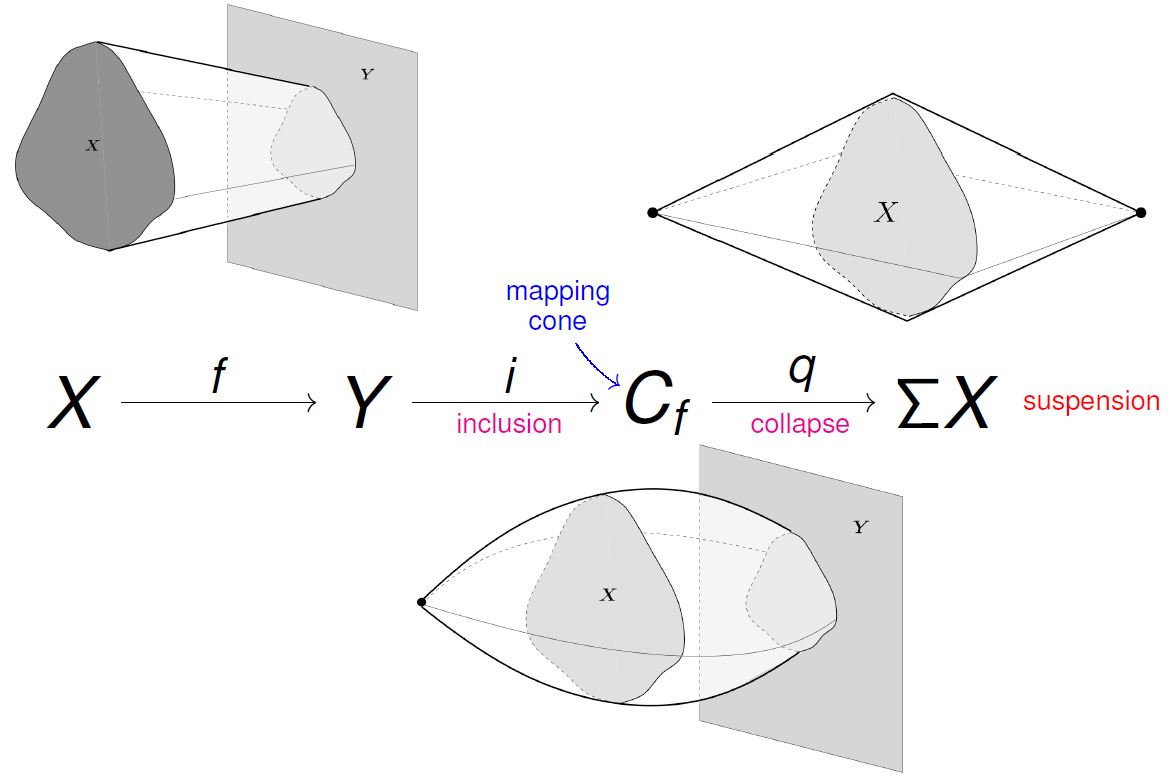
For Top with the standard cyclinder object, def. , then by example , the mapping cone, def. , of a continuous function is obtained by
-
forming the cylinder over ;
-
attaching to one end of that cylinder the space as specified by the map .
-
shrinking the other end of the cylinder to the point.
Accordingly the suspension of a topological space is the result of shrinking both ends of the cylinder on the object two the point. This is homeomoprhic to attaching two copies of the cone on the space at the base of the cone.
(graphics taken from Muro 2010)
Below in example we find the homotopy-theoretic interpretation of this standard topological mapping cone as a model for the homotopy cofiber.
Remark
The formula for the mapping cone in prop. (as opposed to that of the mapping co-cone) does not require the presence of the basepoint: for a morphism in (as opposed to in ) we may still define
where the prime denotes the unreduced cone, formed from a cylinder object in .
Proposition
For a morphism in Top, then its unreduced mapping cone, remark , with respect to the standard cylinder object def. , is isomorphic to the reduced mapping cone, def. , of the morphism (with a basepoint adjoined, def. ) with respect to the standard reduced cylinder (example ):
Proof
By prop. and example , is given by the colimit in over the following diagram:
We may factor the vertical maps to give
This way the top part of the diagram (using the pasting law to compute the colimit in two stages) is manifestly a cocone under the result of applying to the diagram for the unreduced cone. Since is itself given by a colimit, it preserves colimits, and hence gives the partial colimit as shown. The remaining pushout then contracts the remaining copy of the point away.
Example makes it clear that every cycle in that happens to be in the image of can be continuously translated in the cylinder-direction, keeping it constant in , to the other end of the cylinder, where it shrinks away to the point. This means that every homotopy group of , def. , in the image of vanishes in the mapping cone. Hence in the mapping cone the image of under in is removed up to homotopy. This makes it intuitively clear how is a homotopy-version of the cokernel of . We now discuss this formally.
Lemma
Let be a category of cofibrant objects, def. . Then for every morphism the mapping cylinder-construction in def. provides a cofibration resolution of , in that
-
the composite morphism is a cofibration;
-
factors through this morphism by a weak equivalence left inverse to an acyclic cofibration
Dually:
Let be a category of fibrant objects, def. . Then for every morphism the mapping cocylinder-construction in def. provides a fibration resolution of , in that
-
the composite morphism is a fibration;
-
factors through this morphism by a weak equivalence right inverse to an acyclic fibration:
Proof
We discuss the second case. The first case is formally dual.
So consider the mapping cocylinder-construction from prop.
To see that the vertical composite is indeed a fibration, notice that, by the pasting law, the above pullback diagram may be decomposed as a pasting of two pullback diagram as follows
Both squares are pullback squares. Since pullbacks of fibrations are fibrations by prop. , the morphism is a fibration. Similarly, since is fibrant, also the projection map is a fibration (being the pullback of along ).
Since the vertical composite is thereby exhibited as the composite of two fibrations
it is itself a fibration.
Then to see that there is a weak equivalence as claimed:
The universal property of the pullback induces a right inverse of fitting into this diagram
which is a weak equivalence, as indicated, by two-out-of-three (def. ).
This establishes the claim.
Categories of fibrant objects
Below we discuss the homotopy-theoretic properties of the mapping cone- and mapping cocone-constructions from above. Before we do so, we here establish a collection of general facts that hold in categories of fibrant objects and dually in categories of cofibrant objects, def. .
Literature (Brown 73, section 4).
Lemma
Let be a morphism in a category of fibrant objects, def. . Then given any choice of path space objects and , def. , there is a replacement of by a path space object along an acylic fibration, such that has a morphism to which is compatible with the structure maps, in that the following diagram commutes
(Brown 73, section 2, lemma 2)
Proof
Consider the commuting square
Then consider its factorization through the pullback of the right morphism along the bottom morphism,
Finally use the factorization lemma to factor the morphism through a weak equivalence followed by a fibration, the object this factors through serves as the desired path space resolution
Lemma
In a category of fibrant objects , def. , let
be a morphism over some object in and let be any morphism in . Let
be the corresponding morphism pulled back along .
Then
-
if is a fibration then also is a fibration;
-
if is a weak equivalence then also is a weak equivalence.
(Brown 73, section 4, lemma 1)
Proof
For the statement follows from the pasting law which says that if in
the bottom and the total square are pullback squares, then so is the top square. The same reasoning applies for .
Now to see the case that :
Consider the full subcategory of the slice category (def. ) on its fibrant objects, i.e. the full subcategory of the slice category on the fibrations
into . By factorizing for every such fibration the diagonal morphisms into the fiber product through a weak equivalence followed by a fibration, we obtain path space objects relative to :
With these, the factorization lemma (lemma ) applies in .
(Notice that for this we do need the restriction of to the fibrations, because this ensures that the projections are still fibrations, which is used in the proof of the factorization lemma (here).)
So now given any
apply the factorization lemma in to factor it as
By the previous discussion it is sufficient now to show that the base change of to is still a weak equivalence. But by the factorization lemma in , the morphism is right inverse to another acyclic fibration over :
(Notice that if we had applied the factorization lemma of in instead of in then the corresponding triangle on the right here would not commute.)
Now we may reason as before: the base change of the top morphism here is exhibited by the following pasting composite of pullbacks:
The acyclic fibration is preserved by this pullback, as is the identity . Hence the weak equivalence is preserved by two-out-of-three (def. ).
Lemma
In a category of fibrant objects, def. , the pullback of a weak equivalence along a fibration is again a weak equivalence.
(Brown 73, section 4, lemma 2)
Proof
Let be a weak equivalence and be a fibration. We want to show that the left vertical morphism in the pullback
is a weak equivalence.
First of all, using the factorization lemma we may factor as
with the first morphism a weak equivalence that is a right inverse to an acyclic fibration and the right one an acyclic fibration.
Then the pullback diagram in question may be decomposed into two consecutive pullback diagrams
where the morphisms are indicated as fibrations and acyclic fibrations using the stability of these under arbitrary pullback.
This means that the proof reduces to proving that weak equivalences that are right inverse to some acyclic fibration map to a weak equivalence under pullback along a fibration.
Given such with right inverse , consider the pullback diagram
Notice that the indicated universal morphism into the pullback is a weak equivalence by two-out-of-three (def. ).
The previous lemma says that weak equivalences between fibrations over are themselves preserved by base extension along . In total this yields the following diagram
so that with a weak equivalence also is a weak equivalence, as indicated.
Notice that is the morphism that we want to show is a weak equivalence. By two-out-of-three (def. ) for that it is now sufficient to show that is a weak equivalence.
That finally follows now since, by assumption, the total bottom horizontal morphism is the identity. Hence so is the top horizontal morphism. Therefore is right inverse to a weak equivalence, hence is a weak equivalence.
Lemma
Let be a category of fibrant objects, def. in a model structure on pointed objects (prop. ). Given any commuting diagram in of the form
(meaning: both squares commute and equalizes with ) then the localization functor (def. , cor ) takes the morphisms induced by and on fibers (example ) to the same morphism, in the homotopy category.
(Brown 73, section 4, lemma 4)
Proof
First consider the pullback of along : this forms the same kind of diagram but with the bottom morphism an identity. Hence it is sufficient to consider this special case.
Consider the full subcategory of the slice category (def. ) on its fibrant objects, i.e. the full subcategory of the slice category on the fibrations
into . By factorizing for every such fibration the diagonal morphisms into the fiber product through a weak equivalence followed by a fibration, we obtain path space objects relative to :
With these, the factorization lemma (lemma ) applies in .
Let then be a path space object for in the slice over and consider the following commuting square
By factoring this through the pullback and then applying the factorization lemma and then two-out-of-three (def. ) to the factoring morphisms, this may be replaced by a commuting square of the same form, where however the left morphism is an acyclic fibration
This makes also the morphism be a fibration, so that the whole diagram may now be regarded as a diagram in the category of fibrant objects of the slice category over .
As such, the top horizontal morphism now exhibits a right homotopy which under localization (def. ) of the slice model structure (prop. ) we have
The result then follows by observing that we have a commuting square of functors
because, by lemma , the top and right composite sends weak equivalences to isomorphisms, and hence the bottom filler exists by theorem . This implies the claim.
Homotopy fibers
We now discuss the homotopy-theoretic properties of the mapping cone- and mapping cocone-constructions from above.
Literature (Brown 73, section 4).
Remark
The factorization lemma with prop. says that the mapping cocone of a morphism , def. , is equivalently the plain fiber, example , of a fibrant resolution of :
The following prop. says that, up to equivalence, this situation is independent of the specific fibration resolution provided by the factorization lemma (hence by the prescription for the mapping cocone), but only depends on it being some fibration resolution.
Proposition
In the category of fibrant objects , def. , of a model structure on pointed objects (prop. ) consider a morphism of fiber-diagrams, hence a commuting diagram of the form
If and weak equivalences, then so is .
Proof
Factor the diagram in question through the pullback of along
and observe that
-
;
-
is a weak equivalence by assumption and by two-out-of-three (def. );
Moreover, this diagram exhibits as the base change, along , of . Therefore the claim now follows with lemma .
Hence we say:
Definition
Let be a model category and its model category of pointed objects, prop. . For any morphism in its category of fibrant objects , def. , then its homotopy fiber
is the morphism in the homotopy category , def. , which is represented by the fiber, example , of any fibration resolution of (hence any fibration such that factors through a weak equivalence followed by ).
Dually:
For any morphism in its category of cofibrant objects , def. , then its homotopy cofiber
is the morphism in the homotopy category , def. , which is represented by the cofiber, example , of any cofibration resolution of (hence any cofibration such that factors as followed by a weak equivalence).
Proposition
The homotopy fiber in def. is indeed well defined, in that for and two fibration replacements of any morphisms in , then their fibers are isomorphic in .
Proof
It is sufficient to exhibit an isomorphism in from the fiber of the fibration replacement given by the factorization lemma (for any choice of path space object) to the fiber of any other fibration resolution.
Hence given a morphism and a factorization
consider, for any choice of path space object (def. ), the diagram
as in the proof of lemma . Now by repeatedly using prop. :
-
the bottom square gives a weak equivalence from the fiber of to the fiber of ;
-
The square
gives a weak equivalence from the fiber of to the fiber of .
-
Similarly the total vertical composite gives a weak equivalence via
from the fiber of to the fiber of .
Together this is a zig-zag of weak equivalences of the form
between the fiber of and the fiber of . This gives an isomorphism in the homotopy category.
Example
(fibers of Serre fibrations)
In showing that Serre fibrations are abstract fibrations in the sense of model category theory, theorem implies that the fiber (example ) of a Serre fibration, def.
over any point is actually a homotopy fiber in the sense of def. . With prop. this implies that the weak homotopy type of the fiber only depends on the Serre fibration up to weak homotopy equivalence in that if is another Serre fibration fitting into a commuting diagram of the form
then .
In particular this gives that the weak homotopy type of the fiber of a Serre fibration does not change as the basepoint is moved in the same connected component. For let be a path between two points
Then since all objects in are fibrant, and since the endpoint inclusions are weak equivalences, lemma gives the zig-zag of top horizontal weak equivalences in the following diagram:
and hence an isomorphism in the classical homotopy category (def. ).
The same kind of argument applied to maps from the square gives that if are two homotopic paths with coinciding endpoints, then the isomorphisms between fibers over endpoints which they induce are equal. (But in general the isomorphism between the fibers does depend on the choice of homotopy class of paths connecting the basepoints!)
The same kind of argument also shows that if has the structure of a cell complex (def. ) then the restriction of the Serre fibration to one cell may be identified in the homotopy category with , and may be canonically identified so if the fundamental group of is trivial. This is used when deriving the Serre-Atiyah-Hirzebruch spectral sequence for (prop.).
Example
For every continuous function between CW-complexes, def. , then the standard topological mapping cone is the attaching space (example )
of with the standard cone given by collapsing one end of the standard topological cyclinder (def. ) as shown in example .
Equipped with the canonical continuous function
this represents the homotopy cofiber, def. , of with respect to the classical model structure on topological spaces from theorem .
Proof
By prop. , for a CW-complex then the standard topological cylinder object is indeed a cyclinder object in . Therefore by prop. and the factorization lemma , the mapping cone construction indeed produces first a cofibrant replacement of and then the ordinary cofiber of that, hence a model for the homotopy cofiber.
Example
The homotopy fiber of the inclusion of classifying spaces is the n-sphere . See this prop. at Classifying spaces and G-structure.
Example
Suppose a morphism already happens to be a fibration between fibrant objects. The factorization lemma replaces it by a fibration out of the mapping cocylinder , but such that the comparison morphism is a weak equivalence:
Hence by prop. in this case the ordinary fiber of is weakly equivalent to the mapping cocone, def. .
We may now state the abstract version of the statement of prop. :
Proposition
Let be a model category. For any morphism of pointed objects, and for a pointed object, def. , then the sequence
is exact as a sequence of pointed sets.
(Where the sequence here is the image of the homotopy fiber sequence of def. under the hom-functor from example .)
Proof
Let , and denote fibrant-cofibrant objects in representing the given objects of the same name in . Moreover, let be a fibration in representing the given morphism of the same name in .
Then by def. and prop. there is a representative of the homotopy fiber which fits into a pullback diagram of the form
With this the hom-sets in question are represented by genuine morphisms in , modulo homotopy. From this it follows immediately that includes into . Hence it remains to show the converse: that every element in indeed comes from .
But an element in is represented by a morphism such that there is a left homotopy as in the following diagram
Now by lemma the square here has a lift , as shown. This means that is left homotopic to . But by the universal property of the fiber, factors through .
With prop. it also follows notably that the loop space construction becomes well-defined on the homotopy category:
Remark
Given an object , and picking any path space object , def. with induced loop space object , def. , write for the path space object given by the fiber product of with itself, via example . From the pullback diagram there, the fiber inclusion induces a morphism
In the case where and is induced, via def. , from the standard path space object (def. ), i.e. in the case that
then this is the operation of concatenating two loops parameterized by to a single loop parameterized by .
Proposition
Let be a model category, def. . Then the construction of forming loop space objects , def. (which on depends on a choice of path space objects, def. ) becomes unique up to isomorphism in the homotopy category (def. ) of the model structure on pointed objects (prop. ) and extends to a functor:
Dually, the reduced suspension operation, def. , which on depends on a choice of cylinder object, becomes a functor on the homotopy category
Moreover, the pairing operation induced on the objects in the image of this functor via remark (concatenation of loops) gives the objects in the image of group object structure, and makes this functor lift as
(Brown 73, section 4, theorem 3)
Proof
Given an object and given two choices of path space objects and , we need to produce an isomorphism in between and .
To that end, first lemma implies that any two choices of path space objects are connected via a third path space by a span of morphisms compatible with the structure maps. By two-out-of-three (def. ) every morphism of path space objects compatible with the inclusion of the base object is a weak equivalence. With this, lemma implies that these morphisms induce weak equivalences on the corresponding loop space objects. This shows that all choices of loop space objects become isomorphic in the homotopy category.
Moreover, all the isomorphisms produced this way are actually equal: this follows from lemma applied to
This way we obtain a functor
By prop. (and using that Cartesian product preserves weak equivalences) this functor sends weak equivalences to isomorphisms. Therefore the functor on homotopy categories now follows with theorem .
It is immediate to see that the operation of loop concatenation from remark gives the objects the structure of monoids. It is now sufficient to see that these are in fact groups:
We claim that the inverse-assigning operation is given by the left map in the following pasting composite
(where , thus defined, is the path space object obtained from by “reversing the notion of source and target of a path”).
To see that this is indeed an inverse, it is sufficient to see that the two morphisms
induced from
coincide in the homotopy category. This follows with lemma applied to the following commuting diagram:
Homotopy pullbacks
The concept of homotopy fibers of def. is a special case of the more general concept of homotopy pullbacks.
Definition
A model category (def. ) is called
-
a right proper model category if pullback along fibrations preserves weak equivalences;
-
a left proper model category if pushout along cofibrations preserves weak equivalences;
-
a proper model category if it is both left and right proper.
Example
By lemma , a model category (def. ) in which all objects are fibrant is a right proper model category (def. ).
Definition
Let be a right proper model category (def. ). Then a commuting square
in is called a homotopy pullback (of along and equivalently of along ) if the following equivalent conditions hold:
-
for some factorization of the form
the universally induced morphism from into the pullback of along is a weak equivalence:
-
for some factorization of the form
the universally induced morphism from into the pullback of along is a weak equivalence:
-
the above two conditions hold for every such factorization.
(e.g. Goerss-Jardine 96, II (8.14))
Proof
First assume that the first condition holds, in that
Then let
be any factorization of and consider the pasting diagram (using the pasting law for pullbacks)
where the inner morphisms are fibrations and weak equivalences, as shown, by the pullback stability of fibrations (prop. ) and then since pullback along fibrations preserves weak equivalences by assumption of right properness (def. ). Hence it follows by two-out-of-three (def. ) that also the comparison morphism is a weak equivalence.
In conclusion, if the homotopy pullback condition is satisfied for one factorization of , then it is satisfied for all factorizations of . Since the argument is symmetric in and , this proves the claim.
Remark
In particular, an ordinary pullback square of fibrant objects, one of whose edges is a fibration, is a homotopy pullback square according to def. .
Proposition
Let be a right proper model category (def. ). Given a diagram in of the form
then the induced morphism on pullbacks is a weak equivalence
Proof
(The reader should draw the 3-dimensional cube diagram which we describe in words now.)
First consider the universal morphism and observe that it is a weak equivalence by right properness (def. ) and two-out-of-three (def. ).
Then consider the universal morphism and observe that this is also a weak equivalence, since is the limiting cone of a homotopy pullback square by remark , and since the morphism is the comparison morphism to the pullback of the factorization constructed in the first step.
Now by using the pasting law, then the commutativity of the “left” face of the cube, then the pasting law again, one finds that . Again by right properness this implies that is a weak equivalence.
With this the claim follows by two-out-of-three.
Homotopy pullbacks satisfy the usual abstract properties of pullbacks:
Proposition
Let be a right proper model category (def. ). If in a commuting square in one edge is a weak equivalence, then the square is a homotopy pullback square precisely if the opposite edge is a weak equivalence, too.
Proof
Consider a commuting square of the form
To detect whether this is a homotopy pullback, by def. and prop. , we are to choose any factorization of the right vertical morphism to obtain the pasting composite
Here the morphism in the middle is a weak equivalence by right properness (def. ). Hence it follows by two-out-of-three that the top left comparison morphism is a weak equivalence (and so the original square is a homotopy pullback) precisely if the top morphism is a weak equivalence.
Proposition
Let be a right proper model category (def. ).
-
(pasting law) If in a commuting diagram
the square on the right is a homotoy pullback (def. ) then the left square is, too, precisely if the total rectangle is;
-
in the presence of functorial factorization (def. ) through weak equivalences followed by fibrations:
every retract of a homotopy pullback square (in the category of commuting squares in ) is itself a homotopy pullback square.
Proof
For the first statement: choose a factorization of , pull it back to a factorization and assume that is a weak equivalence, i.e. that the right square is a homotopy pullback. Now use the ordinary pasting law to conclude.
For the second statement: functorially choose a factorization of the two right vertical morphisms of the squares and factor the squares through the pullbacks of the corresponding fibrations along the bottom morphisms, respectively. Now the statement that the squares are homotopy pullbacks is equivalent to their top left vertical morphisms being weak equivalences. Factor these top left morphisms functorially as cofibrations followed by acyclic fibrations. Then the statement that the squares are homotopy pullbacks is equivalent to those top left cofibrations being acyclic. Now the claim follows using that the retract of an acyclic cofibration is an acyclic cofibration (prop. ).
Long fiber sequences
The ordinary fiber, example , of a morphism has the property that taking it twice is always trivial:
This is crucially different for the homotopy fiber, def. . Here we discuss how this comes about and what the consequences are.
Proposition
Let be a category of fibrant objects of a model category, def. and let be a morphism in its category of pointed objects, def. . Then the homotopy fiber of its homotopy fiber, def. , is isomorphic, in , to the loop space object of (def. , prop. ):
Proof
Assume without restriction that is already a fibration between fibrant objects in (otherwise replace and rename). Then its homotopy fiber is its ordinary fiber, sitting in a pullback square
In order to compute , i.e. , we need to replace the fiber inclusion by a fibration. Using the factorization lemma for this purpose yields, after a choice of path space object (def. ), a replacement of the form
Hence is the ordinary fiber of this map:
Notice that
because of the pasting law:
Hence
Now we claim that there is a choice of path space objects and such that this model for the homotopy fiber (as an object in ) sits in a pullback diagram of the following form:
By the pasting law and the pullback stability of acyclic fibrations, this will prove the claim.
To see that the bottom square here is indeed a pullback, check the universal property: A morphism out of any into is a morphism and a morphism such that , and . Hence it is equivalently just a morphism such that and . This is the defining universal property of .
Now to construct the right vertical morphism in the top square (Quillen 67, page 3.1): Let be any path space object for and let be given by a factorization
and regarded as a path space object of by further comoposing with
We need to show that is an acyclic fibration.
It is a fibration because is a fibration, this being the pullback of the fibration .
To see that it is also a weak equivalence, first observe that , this being the pullback of the acyclic fibration of lemma . Hence we have a factorization of the identity as
and so finally the claim follows by two-out-of-three (def. ).
Remark
There is a conceptual way to understand prop. as follows: If we draw double arrows to indicate homotopies, then a homotopy fiber (def. ) is depicted by the following filled square:
just like the ordinary fiber (example ) is given by a plain square
One may show that just like the fiber is the universal solution to making such a commuting square (a pullback limit cone def. ), so the homotopy fiber is the universal solution up to homotopy to make such a commuting square up to homotopy – a homotopy pullback homotopy limit cone.
Now just like ordinary pullbacks satisfy the pasting law saying that attaching two pullback squares gives a pullback rectangle, the analogue is true for homotopy pullbacks. This implies that if we take the homotopy fiber of a homotopy fiber, thereby producing this double homotopy pullback square
then the total outer rectangle here is itself a homotopy pullback. But the outer rectangle exhibits the homotopy fiber of the point inclusion, which, via def. and lemma , is the loop space object:
Proposition
(long homotopy fiber sequences)
Let be a model category and let be morphism in the pointed homotopy category (prop. ). Then:
-
There is a long sequence to the left in of the form
where each morphism is the homotopy fiber (def. ) of the following one: the homotopy fiber sequence of . Here denotes followed by forming inverses with respect to the group structure on from prop. .
Moreover, for any object, then there is a long exact sequence
of pointed sets, where denotes the pointed set valued hom-functor of example .
-
Dually, there is a long sequence to the right in of the form
where each morphism is the homotopy cofiber (def. ) of the previous one: the homotopy cofiber sequence of . Moreover, for any object, then there is a long exact sequence
of pointed sets, where denotes the pointed set valued hom-functor of example .
Proof
That there are long sequences of this form is the result of combining prop. and prop. .
It only remains to see that it is indeed the morphisms that appear, as indicated.
In order to see this, it is convenient to adopt the following notation: for a morphism, then we denote the collection of generalized element of its homotopy fiber as
indicating that these elements are pairs consisting of an element of and a “path” (an element of the given path space object) from to the basepoint.
This way the canonical map is . Hence in this notation the homotopy fiber of the homotopy fiber reads
This identifies with by forming the loops
where the overline denotes reversal and the dot denotes concatenation.
Then consider the next homotopy fiber
where on the right we have a path in from to the basepoint element. This is a path together with a path-of-paths which connects to .
By the above convention this is identified with the loop in which is
But the map to sends this data to , hence to the loop
hence to the reveral of the image under of the loop in .
Remark
In (Quillen 67, I.3, prop. 3, prop. 4) more is shown than stated in prop. : there the connecting homomorphism is not just shown to exist, but is described in detail via an action of on in . This takes a good bit more work. For our purposes here, however, it is sufficient to know that such a morphism exists at all, hence that .
Example
Let be the classical model structure on topological spaces (compactly generated) from theorem , theorem . Then using the standard pointed topological path space objects from def. and example as the abstract path space objects in def. , via prop. , this gives that
is the th homotopy group, def. , of at its basepoint.
Hence using in the first item of prop. , the long exact sequence this gives is of the form
This is called the long exact sequence of homotopy groups induced by .
Remark
As we pass to stable homotopy theory (in Part 1)), the long exact sequences in example become long not just to the left, but also to the right. Given then a tower of fibrations, there is an induced sequence of such long exact sequences of homotopy groups, which organizes into an exact couple. For more on this see at Interlude – Spectral sequences (this remark).
Example
Let again be the classical model structure on topological spaces (compactly generated) from theorem , theorem , as in example . For any pointed topological space and an inclusion of pointed topological spaces, the exactness of the sequence in the second item of prop.
gives that the functor
behaves like one degree in an additive reduced cohomology theory (def.). The Brown representability theorem (thm.) implies that all additive reduced cohomology theories are degreewise representable this way (prop.).
-Groupoids I): Topological homotopy theory
This section first recalls relevant concepts from actual topology (“point-set topology”) and highlights facts that motivate the axiomatics of model categories below. We prove two technical lemmas (lemma and lemma ) that serve to establish the abstract homotopy theory of topological spaces further below.
Then we discuss how the category Top of topological spaces satisfies the axioms of abstract homotopy theory (model category) theory, def. .
Literature (Hirschhorn 15)
Throughout, let Top denote the category whose objects are topological spaces and whose morphisms are continuous functions between them. Its isomorphisms are the homeomorphisms.
(Further below we restrict attention to the full subcategory of compactly generated topological spaces.)
Universal constructions
To begin with, we recall some basics on universal constructions in Top: limits and colimits of diagrams of topological spaces; exponential objects.
We now discuss limits and colimits (Def. ) in Top. The key for understanding these is the fact that there are initial and final topologies:
Definition
Let be a set of topological spaces, and let be a bare set. Then
-
For a set of functions out of , the initial topology is the topology on with the minimum collection of open subsets such that all are continuous.
-
For a set of functions into , the final topology is the topology on with the maximum collection of open subsets such that all are continuous.
Example
For a single topological space, and a subset of its underlying set, then the initial topology , def. , is the subspace topology, making
a topological subspace inclusion.
Example
Conversely, for an epimorphism, then the final topology on is the quotient topology.
Proposition
Let be a small category and let be an -diagram in Top (a functor from to ), with components denoted , where and a topology on . Then:
-
The limit of exists and is given by the topological space whose underlying set is the limit in Set of the underlying sets in the diagram, and whose topology is the initial topology, def. , for the functions which are the limiting cone components:
Hence
-
The colimit of exists and is the topological space whose underlying set is the colimit in Set of the underlying diagram of sets, and whose topology is the final topology, def. for the component maps of the colimiting cocone
Hence
(e.g. Bourbaki 71, section I.4)
Proof
The required universal property of (def. ) is immediate: for
any cone over the diagram, then by construction there is a unique function of underlying sets making the required diagrams commute, and so all that is required is that this unique function is always continuous. But this is precisely what the initial topology ensures.
The case of the colimit is formally dual.
Example
The limit over the empty diagram in is the point with its unique topology.
Example
For a set of topological spaces, their coproduct is their disjoint union.
In particular:
Example
For , the -indexed coproduct of the point, is the set itself equipped with the final topology, hence is the discrete topological space on .
Example
For a set of topological spaces, their product is the Cartesian product of the underlying sets equipped with the product topology, also called the Tychonoff product.
In the case that is a finite set, such as for binary product spaces , then a sub-basis for the product topology is given by the Cartesian products of the open subsets of (a basis for) each factor space.
Example
The equalizer of two continuous functions in is the equalizer of the underlying functions of sets
(hence the largets subset of on which both functions coincide) and equipped with the subspace topology, example .
Example
The coequalizer of two continuous functions in is the coequalizer of the underlying functions of sets
(hence the quotient set by the equivalence relation generated by for all ) and equipped with the quotient topology, example .
Example
For
two continuous functions out of the same domain, then the colimit under this diagram is also called the pushout, denoted
(Here is also called the pushout of , or the cobase change of along .)
This is equivalently the coequalizer of the two morphisms from to the coproduct of with (example ):
If is an inclusion, one also writes and calls this the attaching space.
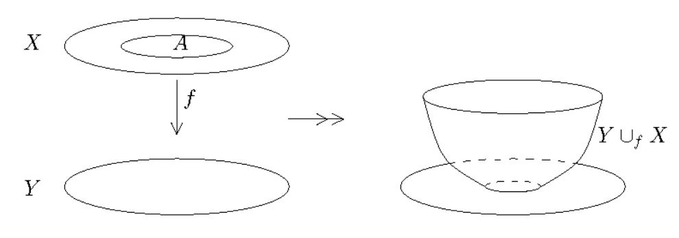
By example the pushout/attaching space is the quotient topological space
of the disjoint union of and subject to the equivalence relation which identifies a point in with a point in if they have the same pre-image in .
(graphics from Aguilar-Gitler-Prieto 02)
Notice that the defining universal property of this colimit means that completing the span
to a commuting square
is equivalent to finding a morphism
Example
For a topological subspace inclusion, example , then the pushout
is the quotient space or cofiber, denoted .
Example
An important special case of example :
For write
-
for the standard topological n-disk (equipped with its subspace topology as a subset of Cartesian space);
Notice that and that .
Let
be the canonical inclusion of the standard (n-1)-sphere as the boundary of the standard n-disk (both regarded as topological spaces with their subspace topology as subspaces of the Cartesian space ).
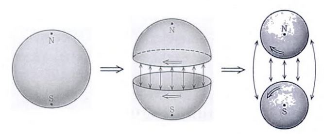
Then the colimit in Top under the diagram
i.e. the pushout of along itself, is the n-sphere :
(graphics from Ueno-Shiga-Morita 95)
Another kind of colimit that will play a role for certain technical constructions is transfinite composition. First recall
Definition
A partial order is a set equipped with a relation such that for all elements
1) (reflexivity) ;
2) (transitivity) if and then ;
3) (antisymmetry) if and then .
This we may and will equivalently think of as a category with objects the elements of and a unique morphism precisely if . In particular an order-preserving function between partially ordered sets is equivalently a functor between their corresponding categories.
A bottom element in a partial order is one such that for all a. A top element is one for wich .
A partial order is a total order if in addition
4) (totality) either or .
A total order is a well order if in addition
5) (well-foundedness) every non-empty subset has a least element.
An ordinal is the equivalence class of a well-order.
The successor of an ordinal is the class of the well-order with a top element freely adjoined.
A limit ordinal is one that is not a successor.
Example
The finite ordinals are labeled by , corresponding to the well-orders . Here is the successor of . The first non-empty limit ordinal is .
Definition
Let be a category, and let be a class of its morphisms.
For an ordinal (regarded as a category), an -indexed transfinite sequence of elements in is a diagram
such that
-
takes all successor morphisms in to elements in
-
is continuous in that for every nonzero limit ordinal , restricted to the full-subdiagram is a colimiting cocone in for restricted to .
The corresponding transfinite composition is the induced morphism
into the colimit of the diagram, schematically:
We now turn to the discussion of mapping spaces/exponential objects.
Definition
For a topological space and a locally compact topological space (in that for every point, every neighbourhood contains a compact neighbourhood), the mapping space
is the topological space
-
whose underlying set is the set of continuous functions ,
-
whose open subsets are unions of finitary intersections of the following subbase elements of standard open subsets:
the standard open subset for
-
a compact topological space subset
-
an open subset
is the subset of all those continuous functions that fit into a commuting diagram of the form
-
Accordingly this is called the compact-open topology on the set of functions.
The construction extends to a functor
Proposition
For a topological space and a locally compact topological space (in that for each point, each open neighbourhood contains a compact neighbourhood), the topological mapping space from def. is an exponential object, i.e. the functor is right adjoint to the product functor : there is a natural bijection
between continuous functions out of any product topological space of with any and continuous functions from into the mapping space.
A proof is spelled out here (or see e.g. Aguilar-Gitler-Prieto 02, prop. 1.3.1).
Remark
In the context of prop. it is often assumed that is also a Hausdorff topological space. But this is not necessary. What assuming Hausdorffness only achieves is that all alternative definitions of “locally compact” become equivalent to the one that is needed for the proposition: for every point, every open neighbourhood contains a compact neighbourhood.
Remark
Proposition fails in general if is not locally compact. Therefore the plain category Top of all topological spaces is not a Cartesian closed category.
This is no problem for the construction of the homotopy theory of topological spaces as such, but it becomes a technical nuisance for various constructions that one would like to perform within that homotopy theory. For instance on general pointed topological spaces the smash product is in general not associative.
On the other hand, without changing any of the following discussion one may just pass to a more convenient category of topological spaces such as notably the full subcategory of compactly generated topological spaces (def. ) which is Cartesian closed. This we turn to below.
Homotopy
The fundamental concept of homotopy theory is clearly that of homotopy. In the context of topological spaces this is about contiunous deformations of continuous functions parameterized by the standard interval:
Definition
Write
for the standard topological interval, a compact connected topological subspace of the real line.
Equipped with the canonical inclusion of its two endpoints
this is the standard interval object in Top.
For , the product topological space , example , is called the standard cylinder object over . The endpoint inclusions of the interval make it factor the codiagonal on
Definition
For two continuous functions between topological spaces , then a left homotopy
is a continuous function
out of the standard cylinder object over , def. , such that this fits into a commuting diagram of the form
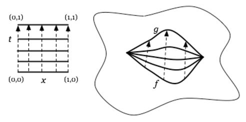
(graphics grabbed from J. Tauber here)
Example
Let be a topological space and let be two of its points, regarded as functions from the point to . Then a left homotopy, def. , between these two functions is a commuting diagram of the form
This is simply a continuous path in whose endpoints are and .
For instance:
Example
Let
be the continuous function from the standard interval to itself that is constant on the value 0. Then there is a left homotopy, def. , from the identity function
given by
A key application of the concept of left homotopy is to the definition of homotopy groups:
Definition
For a topological space, then its set of connected components, also called the 0-th homotopy set, is the set of left homotopy-equivalence classes (def. ) of points , hence the set of path-connected components of (example ). By composition this extends to a functor
For , and for any point, then the th homotopy group of at is the group
-
whose underlying set is the set of left homotopy-equivalence classes of maps that take the boundary of to and where the left homotopies are constrained to be constant on the boundary;
-
whose group product operation takes and to with
where the first map is a homeomorphism from the unit -cube to the -cube with one side twice the unit length (e.g. ).
By composition, this construction extends to a functor
from pointed topological spaces to graded groups.
Notice that often one writes the value of this functor on a morphism as .
Remark
At this point we don’t go further into the abstract reason why def. yields group structure above degree 0, which is that positive dimension spheres are H-cogroup objects. But this is important, for instance in the proof of the Brown representability theorem. See the section Brown representability theorem in Part S.
Definition
A continuous function is called a homotopy equivalence if there exists a continuous function the other way around, , and left homotopies, def. , from the two composites to the identity:
and
If here is constant along , is said to exhibit as a deformation retract of .
Example
For a topological space and its standard cylinder object of def. , then the projection and the inclusion are homotopy equivalences, def. , and in fact are homotopy inverses to each other:
The composition
is immediately the identity on (i.e. homotopic to the identity by a trivial homotopy), while the composite
is homotopic to the identity on by a homotopy that is pointwise in that of example .
Definition
A continuous function is called a weak homotopy equivalence if its image under all the homotopy group functors of def. is an isomorphism, hence if
and for all and all
Proposition
Every homotopy equivalence, def. , is a weak homotopy equivalence, def. .
In particular a deformation retraction, def. , is a weak homotopy equivalence.
Proof
First observe that for all Top the inclusion maps
into the standard cylinder object, def. , are weak homotopy equivalences: by postcomposition with the contracting homotopy of the interval from example all homotopy groups of have representatives that factor through this inclusion.
Then given a general homotopy equivalence, apply the homotopy groups functor to the corresponding homotopy diagrams (where for the moment we notationally suppress the choice of basepoint for readability) to get two commuting diagrams
By the previous observation, the vertical morphisms here are isomorphisms, and hence these diagrams exhibit as the inverse of , hence both as isomorphisms.
Remark
The converse of prop. is not true generally: not every weak homotopy equivalence between topological spaces is a homotopy equivalence. (For an example with full details spelled out see for instance Fritsch, Piccinini: “Cellular Structures in Topology”, p. 289-290).
However, as we will discuss below, it turns out that
-
every weak homotopy equivalence between CW-complexes is a homotopy equivalence (Whitehead's theorem, cor. );
-
every topological space is connected by a weak homotopy equivalence to a CW-complex (CW approximation, remark ).
Example
For , the projection from the cylinder object of , def. , is a weak homotopy equivalence, def. . This means that the factorization
of the codiagonal in def. , which in general is far from being a monomorphism, may be thought of as factoring it through a monomorphism after replacing , up to weak homotopy equivalence, by .
In fact, further below (prop. ) we see that has better properties than the generic monomorphism has, in particular better homotopy invariant properties: it has the left lifting property against all Serre fibrations that are also weak homotopy equivalences.
Of course the concept of left homotopy in def. is accompanied by a concept of right homotopy. This we turn to now.
Definition
For a topological space, its standard topological path space object is the topological path space, hence the mapping space , prop. , out of the standard interval of def. .
Example
The endpoint inclusion into the standard interval, def. , makes the path space of def. factor the diagonal on through the inclusion of constant paths and the endpoint evaluation of paths:
This is the formal dual to example . As in that example, below we will see (prop. ) that this factorization has good properties, in that
-
is a Serre fibration.
So while in general the diagonal is far from being an epimorphism or even just a Serre fibration, the factorization through the path space object may be thought of as replacing , up to weak homotopy equivalence, by its path space, such as to turn its diagonal into a Serre fibration after all.
Definition
For two continuous functions between topological spaces , then a right homotopy is a continuous function
into the path space object of , def. , such that this fits into a commuting diagram of the form
Cell complexes
We consider topological spaces that are built consecutively by attaching basic cells.
Definition
Write
for the set of canonical boundary inclusion maps of the standard n-disks, example . This going to be called the set of standard topological generating cofibrations.
Definition
For and for , an -cell attachment to is the pushout (“attaching space”, example ) of a generating cofibration, def.
along some continuous function .
A continuous function is called a topological relative cell complex if it is exhibited by a (possibly infinite) sequence of cell attachments to , in that it is a transfinite composition (def. ) of pushouts (example )
of coproducts (example ) of generating cofibrations (def. ).
A topological space is a cell complex if is a relative cell complex.
A relative cell complex is called a finite relative cell complex if it is obtained from a finite number of cell attachments.
A (relative) cell complex is called a (relative) CW-complex if the above transfinite composition is countable
and if is obtained from by attaching cells precisely only of dimension .
Remark
Strictly speaking a relative cell complex, def. , is a function , together with its cell structure, hence together with the information of the pushout diagrams and the transfinite composition of the pushout maps that exhibit it.
In many applications, however, all that matters is that there is some (relative) cell decomosition, and then one tends to speak loosely and mean by a (relative) cell complex only a (relative) topological space that admits some cell decomposition.
The following lemma , together with lemma below are the only two statements of the entire development here that involve the concrete particular nature of topological spaces (“point-set topology”), everything beyond that is general abstract homotopy theory.
Lemma
Assuming the axiom of choice and the law of excluded middle, every compact subspace of a topological cell complex, def. , intersects the interior of a finite number of cells.
(e.g. Hirschhorn 15, section 3.1)
Proof
So let be a topological cell complex and a compact subspace. Define a subset
by choosing one point in the interior of the intersection with of each cell of that intersects .
It is now sufficient to show that has no accumulation point. Because, by the compactness of , every non-finite subset of does have an accumulation point, and hence the lack of such shows that is a finite set and hence that intersects the interior of finitely many cells of .
To that end, let be any point. If is a 0-cell in , write . Otherwise write for the unique cell of that contains in its interior. By construction, there is exactly one point of in the interior of . Hence there is an open neighbourhood containing no further points of beyond possibly itself, if happens to be that single point of in .
It is now sufficient to show that may be enlarged to an open subset of containing no point of , except for possibly itself, for that means that is not an accumulation point of .
To that end, let be the ordinal that labels the stage of the transfinite composition in the cell complex-presentation of at which the cell above appears. Let be the ordinal of the full cell complex. Then define the set
and regard this as a partially ordered set by declaring a partial ordering via
This is set up such that every element of with the maximum value is an extension that we are after.
Observe then that for a chain in (a subset on which the relation restricts to a total order), it has an upper bound in given by the union . Therefore Zorn's lemma applies, saying that contains a maximal element .
Hence it is now sufficient to show that . We argue this by showing that assuming leads to a contradiction.
So assume . Then to construct an element of that is larger than , consider for each cell at stage its attaching map and the corresponding preimage open set . Enlarging all these preimages to open subsets of (such that their image back in does not contain ), then . This is a contradiction. Hence , and we are done.
It is immediate and useful to generalize the concept of topological cell complexes as follows.
Definition
For any category and for any sub-class of its morphisms, a relative -cell complexes is a morphism in which is a transfinite composition (def. ) of pushouts of coproducts of morphsims in .
Definition
Write
for the set of inclusions of the topological n-disks, def. , into their cylinder objects, def. , along (for definiteness) the left endpoint inclusion.
These inclusions are similar to the standard topological generating cofibrations of def. , but in contrast to these they are “acyclic” (meaning: trivial on homotopy classes of maps from “cycles” given by n-spheres) in that they are weak homotopy equivalences (by prop. ).
Accordingly, is to be called the set of standard topological generating acyclic cofibrations.
Lemma
For a CW-complex (def. ), then its inclusion into its standard cylinder (def. ) is a -relative cell complex (def. , def. ).
Proof
First erect a cylinder over all 0-cells
Assume then that the cylinder over all -cells of has been erected using attachment from . Then the union of any -cell of with the cylinder over its boundary is homeomorphic to and is like the cylinder over the cell “with end and interior removed”. Hence via attaching along the cylinder over is erected.
Lemma
The maps in def. are finite relative cell complexes, def. . In other words, the elements of are -relative cell complexes.
Proof
There is a homeomorphism
such that the map on the right is the inclusion of one hemisphere into the boundary n-sphere of . This inclusion is the result of attaching two cells:
Lemma
Every -relative cell complex (def. , def. ) is a weak homotopy equivalence, def. .
Proof
Let be a -relative cell complex.
First observe that with the elements of being homotopy equivalences for all (by example ), each of the stages in the relative cell complex is also a homotopy equivalence. We make this fully explicit:
By definition, such a stage is a pushout of the form
Then the fact that the projections are strict left inverses to the inclusions gives a commuting square of the form
and so the universal property of the colimit (pushout) gives a factorization of the identity morphism on the right through
which exhibits as a strict left inverse to . Hence it is now sufficient to show that this is also a homotopy right inverse.
To that end, let
be the left homotopy that exhibits as a homotopy right inverse to by example . For each consider the commuting square
Regarded as a cocone under the span in the top left, the universal property of the colimit (pushout) gives a continuous function
for each . For this construction reduces to the provious one in that is the composite which we need to homotope to the identity; while is the identity. Since is clearly also continuous in it constitutes a continuous function
which exhibits the required left homotopy.
So far this shows that each stage in the transfinite composition defining is a homotopy equivalence, hence, by prop. , a weak homotopy equivalence.
This means that all morphisms in the following diagram (notationally suppressing basepoints and showing only the finite stages)
are isomorphisms.
Moreover, lemma gives that every representative and every null homotopy of elements in already exists at some finite stage . This means that also the universally induced morphism
is an isomorphism. Hence the composite is an isomorphism.
Fibrations
Given a relative -cell complex , def. , it is typically interesting to study the extension problem along , i.e. to ask which topological spaces are such that every continuous function has an extension along
If such extensions exists, it means that is sufficiently “spread out” with respect to the maps in . More generally one considers this extension problem fiberwise, i.e. with both and (hence also ) equipped with a map to some base space :
Definition
Given a category and a sub-class of its morphisms, then a morphism in is said to have the right lifting property against the morphisms in if every commuting diagram in of the form
with , has a lift , in that it may be completed to a commuting diagram of the form
We will also say that is a -injective morphism if it satisfies the right lifting property against .
Definition
A continuous function is called a Serre fibration if it is a -injective morphism; i.e. if it has the right lifting property, def. , against all topological generating acylic cofibrations, def. ; hence if for every commuting diagram of continuous functions of the form
has a lift , in that it may be completed to a commuting diagram of the form
Remark
Def. says, in view of the definition of left homotopy, that a Serre fibration is a map with the property that given a left homotopy, def. , between two functions into its codomain, and given a lift of one the two functions through , then also the homotopy between the two lifts. Therefore the condition on a Serre fibration is also called the homotopy lifting property for maps whose domain is an n-disk.
More generally one may ask functions to have such homotopy lifting property for functions with arbitrary domain. These are called Hurewicz fibrations.
Remark
The precise shape of and in def. turns out not to actually matter much for the nature of Serre fibrations. We will eventually find below (prop. ) that what actually matters here is only that the inclusions are relative cell complexes (lemma ) and weak homotopy equivalences (prop. ) and that all of these may be generated from them in a suitable way.
But for simple special cases this is readily seen directly, too. Notably we could replace the n-disks in def. with any homeomorphic topological space. A choice important in the comparison to the classical model structure on simplicial sets (below) is to instead take the topological n-simplices . Hence a Serre fibration is equivalently characterized as having lifts in all diagrams of the form
Other deformations of the -disks are useful in computations, too. For instance there is a homeomorphism from the -disk to its “cylinder with interior and end removed”, formally:
and hence is a Serre fibration equivalently also if it admits lifts in all diagrams of the form
The following is a general fact about closure of morphisms defined by lifting properties which we prove in generality below as prop. .
Proposition
A Serre fibration, def. has the right lifting property against all retracts (see remark ) of -relative cell complexes (def. , def. ).
The following statement is foreshadowing the long exact sequences of homotopy groups (below) induced by any fiber sequence, the full version of which we come to below (example ) after having developed more of the abstract homotopy theory.
Proposition
Let be a Serre fibration, def. , let be any point and write
for the fiber inclusion over that point. Then for every choice of lift of the point through , the induced sequence of homotopy groups
is exact, in that the kernel of is canonically identified with the image of :
Proof
It is clear that the image of is in the kernel of (every sphere in becomes constant on , hence contractible, when sent forward to ).
For the converse, let be represented by some . Assume that is in the kernel of . This means equivalently that fits into a commuting diagram of the form
where is the contracting homotopy witnessing that .
Now since is a lift of , there exists a left homotopy
as follows:
(for instance: regard as embedded in such that is identified with the basepoint on the boundary of and set ).
The pasting of the top two squares that have appeared this way is equivalent to the following commuting square
Because is a Serre fibration and by lemma and prop. , this has a lift
Notice that is a basepoint preserving left homotopy from to some . Being homotopic, they represent the same element of :
But the new representative has the special property that its image in is not just trivializable, but trivialized: combining with the previous diagram shows that it sits in the following commuting diagram
The commutativity of the outer square says that is constant, hence that is entirely contained in the fiber . Said more abstractly, the universal property of fibers gives that factors through , hence that is in the image of .
The following lemma , together with lemma above, are the only two statements of the entire development here that crucially involve the concrete particular nature of topological spaces (“point-set topology”), everything beyond that is general abstract homotopy theory.
Lemma
The continuous functions with the right lifting property, def. against the set of topological generating cofibrations, def. , are precisely those which are both weak homotopy equivalences, def. as well as Serre fibrations, def. .
Proof
We break this up into three sub-statements:
A) -injective morphisms are in particular weak homotopy equivalences
Let have the right lifting property against
We check that the lifts in these diagrams exhibit as being an isomorphism on all homotopy groups, def. :
For the existence of these lifts says that every point of is in the image of , hence that is surjective. Let then be a map that hits two connected components, then the existence of the lift says that if they have the same image in then they were already the same connected component in . Hence is also injective and hence is a bijection.
Similarly, for , if represents an element in that becomes trivial in , then the existence of the lift says that it already represented the trivial element itself. Hence has trivial kernel and so is injective.
Finally, to see that is also surjective, hence bijective, observe that every elements in is equivalently represented by a commuting diagram of the form
and so here the lift gives a representative of a preimage in .
B) -injective morphisms are in particular Serre fibrations
By an immediate closure property of lifting problems (we spell this out in generality as prop. , cor. below) an -injective morphism has the right lifting property against all relative cell complexes, and hence, by lemma , it is also a -injective morphism, hence a Serre fibration.
C) Acyclic Serre fibrations are in particular -injective morphisms
Let be a Serre fibration that induces isomorphisms on homotopy groups. In degree 0 this means that is an isomorphism on connected components, and this means that there is a lift in every commuting square of the form
(this is being surjective) and in every commuting square of the form
(this is being injective). Hence we are reduced to showing that for every diagram of the form
has a lift.
To that end, pick a basepoint on and write and for its images in and , respectively
Then the diagram above expresses that and hence by assumption on it follows that , which in turn mean that there is making the upper triangle of our lifting problem commute:
It is now sufficient to show that any such may be deformed to a which keeps making this upper triangle commute but also makes the remaining lower triangle commute.
To that end, notice that by the commutativity of the original square, we already have at least this commuting square:
This induces the universal map from the pushout of its cospan in the top left, which is the n-sphere (see this example):
This universal morphism represents an element of the th homotopy group:
By assumption that is a weak homotopy equivalence, there is a with
hence on representatives there is a lift up to homotopy
Morever, we may always find of the form for some . (“Paste to the reverse of .”)
Consider then the map
and observe that this represents the trivial class:
This means equivalently that there is a homotopy
fixing the boundary of the -disk.
Hence if we denote homotopy by double arrows, then we have now achieved the following situation
and it now suffices to show that may be lifted to a homotopy of just , fixing the boundary, for then the resulting homotopic is the desired lift.
To that end, notice that the condition that fixes the boundary of the -disk means equivalently that it extends to a morphism
out of the pushout that identifies in the cylinder over all points lying over the boundary. Hence we are reduced to finding a lift in
But inspection of the left map reveals that it is homeomorphic again to , and hence the lift does indeed exist.
The classical model structure on topological spaces
Definition
Say that a continuous function, hence a morphism in Top, is
-
a classical weak equivalence if it is a weak homotopy equivalence, def. ;
-
a classical fibration if it is a Serre fibration, def. ;
-
a classical cofibration if it is a retract (rem. ) of a relative cell complex, def. .
and hence
-
a acyclic classical cofibration if it is a classical cofibration as well as a classical weak equivalence;
-
a acyclic classical fibration if it is a classical fibration as well as a classical weak equivalence.
Write
for the classes of these morphisms, respectively.
We first prove now that the classes of morphisms in def. satisfy the conditions for a model category structure, def. (after some lemmas, this is theorem below). Then we discuss the resulting classical homotopy category (below) and then a few variant model structures whose proof follows immediately along the line of the proof of :
-
The model structure on compactly generated topological spaces and ;
-
The model structure on topologically enriched functors and .
Proposition
The classical weak equivalences, def. , satify two-out-of-three (def. ).
Proof
Since isomorphisms (of homotopy groups) satisfy 2-out-of-3, this property is directly inherited via the very definition of weak homotopy equivalence, def. .
Lemma
Every morphism in Top factors as a classical cofibration followed by an acyclic classical fibration, def. :
Proof
By lemma the set of topological generating cofibrations, def. , has small domains, in the sense of def. (the n-spheres are compact). Hence by the small object argument, prop. , factors as an -relative cell complex, def. , hence just a plain relative cell complex, def. , followed by an -injective morphisms, def. :
By lemma the map is both a weak homotopy equivalence as well as a Serre fibration.
Lemma
Every morphism in Top factors as an acyclic classical cofibration followed by a fibration, def. :
Proof
By lemma the set of topological generating acyclic cofibrations, def. , has small domains, in the sense of def. (the n-disks are compact). Hence by the small object argument, prop. , factors as an -relative cell complex, def. , followed by a -injective morphisms, def. :
By definition this makes a Serre fibration, hence a fibration.
By lemma a relative -cell complex is in particular a relative -cell complex. Hence is a classical cofibration. By lemma it is also a weak homotopy equivalence, hence a clasical weak equivalence.
Lemma
Every commuting square in Top with the left morphism a classical cofibration and the right morphism a fibration, def.
admits a lift as soon as one of the two is also a classical weak equivalence.
Proof
A) If the fibration is also a weak equivalence, then lemma says that it has the right lifting property against the generating cofibrations , and cor. implies the claim.
B) If the cofibration on the left is also a weak equivalence, consider any factorization into a relative -cell complex, def. , def. , followed by a fibration,
as in the proof of lemma . By lemma the morphism is a weak homotopy equivalence, and so by two-out-of-three (prop. ) the factorizing fibration is actually an acyclic fibration. By case A), this acyclic fibration has the right lifting property against the cofibration itself, and so the retract argument, lemma gives that is a retract of a relative -cell complex. With this, finally cor. implies that has the right lifting property against .
Finally:
Proposition
The systems and from def. are weak factorization systems.
Proof
Since we have already seen the factorization property (lemma , lemma ) and the lifting properties (lemma ), it only remains to see that the given left/right classes exhaust the class of morphisms with the given lifting property.
For the classical fibrations this is by definition, for the the classical acyclic fibrations this is by lemma .
The remaining statement for and follows from a general argument (here) for cofibrantly generated model categories (def. ), which we spell out:
So let be in , we need to show that then is a retract (remark ) of a relative cell complex. To that end, apply the small object argument as in lemma to factor as
It follows that has the left lifting property against , and hence by the retract argument (lemma ) it is a retract of . This proves the claim for .
The analogous argument for , using the small object argument for , shows that every is a retract of a -cell complex. By lemma and lemma a -cell complex is both an -cell complex and a weak homotopy equivalence. Retracts of the former are cofibrations by definition, and retracts of the latter are still weak homotopy equivalences by lemma . Hence such is an acyclic cofibration.
In conclusion, prop. and prop. say that:
Theorem
The classes of morphisms in of def. ,
define a model category structure (def. ) , the classical model structure on topological spaces or Serre-Quillen model structure .
In particular
-
every object in is fibrant;
-
the cofibrant objects in are the retracts of cell complexes.
Hence in particular the following classical statement is an immediate corollary:
Corollary
(Whitehead theorem)
Every weak homotopy equivalence (def. ) between topological spaces that are homeomorphic to a retract of a cell complex, in particular to a CW-complex (def. ), is a homotopy equivalence (def. ).
In proving theorem we have in fact shown a bit more that stated. Looking back, all the structure of is entirely induced by the set (def. ) of generating cofibrations and the set (def. ) of generating acyclic cofibrations (whence the terminology). This situation is usefully summarized by the concept of cofibrantly generated model category (Def. ).
This phenomenon will keep recurring and will keep being useful as we construct further model categories, such as the classical model structure on pointed topological spaces (def. ), the projective model structure on topological functors (thm. ), and finally various model structures on spectra which we turn to in the section on stable homotopy theory.
The classical homotopy category
With the classical model structure on topological spaces in hand, we now have good control over the classical homotopy category:
Definition
The Serre-Quillen classical homotopy category is the homotopy category, def. , of the classical model structure on topological spaces from theorem : we write
Remark
From just theorem , the definition (def. ) gives that
is the category whose objects are retracts of cell complexes (def. ) and whose morphisms are homotopy classes of continuous functions. But in fact more is true:
Theorem in itself implies that every topological space is weakly equivalent to a retract of a cell complex, def. . But by the existence of CW approximations, this cell complex may even be taken to be a CW complex.
(Better yet, there is Quillen equivalence to the classical model structure on simplicial sets which implies a functorial CW approximation given by forming the geometric realization of the singular simplicial complex of .)
Hence the Serre-Quillen classical homotopy category is also equivalently the category of just the CW-complexes whith homotopy classes of continuous functions between them
It follows that the universal property of the homotopy category (theorem )
implies that there is a bijection, up to natural isomorphism, between
-
functors out of which agree on homotopy-equivalent maps;
-
functors out of all of which send weak homotopy equivalences to isomorphisms.
This statement in particular serves to show that two different axiomatizations of generalized (Eilenberg-Steenrod) cohomology theories are equivalent to each other. See at Introduction to Stable homotopy theory – S the section generalized cohomology functors (this prop.)
Beware that, by remark , what is not equivalent to is the category
obtained from all topological spaces with morphisms the homotopy classes of continuous functions. This category is “too large”, the correct homotopy category is just the genuine full subcategory
Beware also the ambiguity of terminology: “classical homotopy category” some literature refers to instead of . However, here we never have any use for and will not mention it again.
Proposition
Let be a CW-complex, def. . Then the standard topological cylinder of def.
(obtained by forming the product space with the standard topological interval ) is indeed a cylinder object in the abstract sense of def. .
Proof
We describe the proof informally. It is immediate how to turn this into a formal proof, but the notation becomes tedious. (One place where it is spelled out completely is Ottina 14, prop. 2.9.)
So let be a presentation of as a CW-complex. Proceed by induction on the cell dimension.
First observe that the cylinder over is a cell complex: First itself is a disjoint union of points. Adding a second copy for every point (i.e. attaching along ) yields , then attaching an inteval between any two corresponding points (along ) yields .
So assume that for it has been shown that has the structure of a CW-complex of dimension . Then for each cell of , attach it twice to , once at , and once at .
The result is with a hollow cylinder erected over each of its -cells. Now fill these hollow cylinders (along ) to obtain .
This completes the induction, hence the proof of the CW-structure on .
The construction also manifestly exhibits the inclusion as a relative cell complex.
Finally, it is clear (prop. ) that is a weak homotopy equivalence.
Conversely:
Proposition
Let be any topological space. Then the standard topological path space object (def. )
(obtained by forming the mapping space, def. , with the standard topological interval ) is indeed a path space object in the abstract sense of def. .
Proof
To see that is a weak homotopy equivalence it is sufficient, by prop. , to exhibit a homotopy equivalence. Let the homotopy inverse be . Then the composite
is already equal to the identity. The other we round, the rescaling of paths provides the required homotopy
To see that is a fibration, we need to show that every commuting square of the form
has a lift.
Now first use the adjunction from prop. to rewrite this equivalently as the following commuting square:
This square is equivalently (example ) a morphism out of the pushout
By the same reasoning, a lift in the original diagram is now equivalently a lifting in
Inspection of the component maps shows that the left vertical morphism here is the inclusion into the square times of three of its faces times . This is homeomorphic to the inclusion (as in remark ). Therefore a lift in this square exsists, and hence a lift in the original square exists.
Model structure on pointed spaces
A pointed object is of course an object equipped with a point , and a morphism of pointed objects is a morphism that takes to . Trivial as this is in itself, it is good to record some basic facts, which we do here.
Passing to pointed objects is also the first step in linearizing classical homotopy theory to stable homotopy theory. In particular, every category of pointed objects has a zero object, hence has zero morphisms. And crucially, if the original category had Cartesian products, then its pointed objects canonically inherit a non-cartesian tensor product: the smash product. These ingredients will be key below in the section on stable homotopy theory.
Definition
Let be a category and let be an object.
The slice category is the category whose
-
objects are morphisms in ;
-
morphisms are commuting triangles in .
Dually, the coslice category is the category whose
-
objects are morphisms in ;
-
morphisms are commuting triangles in .
There are the canonical forgetful functors
given by forgetting the morphisms to/from .
We here focus on this class of examples:
Definition
For a category with terminal object , the coslice category (def. ) is the corresponding category of pointed objects: its
-
objects are morphisms in of the form (hence an object equipped with a choice of point; i.e. a pointed object);
-
morphisms are commuting triangles of the form
(hence morphisms in which preserve the chosen points).
Remark
In a category of pointed objects , def. , the terminal object coincides with the initial object, both are given by itself, pointed in the unique way.
In this situation one says that is a zero object and that is a pointed category.
It follows that also all hom-sets of are canonically pointed sets, pointed by the zero morphism
Definition
Let be a category with terminal object and finite colimits. Then the forgetful functor from its category of pointed objects, def. , has a left adjoint
given by forming the disjoint union (coproduct) with a base point (“adjoining a base point”).
Proposition
Let be a category with all limits and colimits. Then also the category of pointed objects , def. , has all limits and colimits.
Moreover:
-
the limits are the limits of the underlying diagrams in , with the base point of the limit induced by its universal property in ;
-
the colimits are the limits in of the diagrams with the basepoint adjoined.
Proof
It is immediate to check the relevant universal property. For details see at slice category – limits and colimits.
Example
Given two pointed objects and , then:
-
their product in is simply ;
-
their coproduct in has to be computed using the second clause in prop. : since the point has to be adjoined to the diagram, it is given not by the coproduct in , but by the pushout in of the form:
This is called the wedge sum operation on pointed objects.
Generally for a set in
Example
For a CW-complex, def. then for every the quotient (example ) of its -skeleton by its -skeleton is the wedge sum, def. , of -spheres, one for each -cell of :
Definition
For a category of pointed objects with finite limits and finite colimits, the smash product is the functor
given by
hence by the pushout in
In terms of the wedge sum from def. , this may be written concisely as
Remark
For a general category in def. , the smash product need not be associative, namely it fails to be associative if the functor does not preserve the quotients involved in the definition.
In particular this may happen for Top.
A sufficient condition for to preserve quotients is that it is a left adjoint functor. This is the case in the smaller subcategory of compactly generated topological spaces, we come to this in prop. below.
These two operations are going to be ubiquituous in stable homotopy theory:
| symbol | name | category theory |
|---|---|---|
| wedge sum | coproduct in | |
| smash product | tensor product in |
Example
Let be pointed topological spaces. Then
denotes the standard interval object from def. , with a djoint basepoint adjoined, def. . Now for any pointed topological space, then
is the reduced cylinder over : the result of forming the ordinary cyclinder over as in def. , and then identifying the interval over the basepoint of with the point.
(Generally, any construction in properly adapted to pointed objects is called the “reduced” version of the unpointed construction. Notably so for “reduced suspension” which we come to below.)
Just like the ordinary cylinder receives a canonical injection from the coproduct formed in , so the reduced cyclinder receives a canonical injection from the coproduct formed in , which is the wedge sum from example :
Example
For pointed topological spaces with a locally compact topological space, then the pointed mapping space is the topological subspace of the mapping space of def.
on those maps which preserve the basepoints, and pointed by the map constant on the basepoint of .
In particular, the standard topological pointed path space object on some pointed (the pointed variant of def. ) is the pointed mapping space .
The pointed consequence of prop. then gives that there is a natural bijection
between basepoint-preserving continuous functions out of a smash product, def. , with pointed continuous functions of one variable into the pointed mapping space.
Example
Given a morphism in a category of pointed objects , def. , with finite limits and colimits,
Remark
In the situation of example , both the pullback as well as the pushout are equivalently computed in . For the pullback this is the first clause of prop. . The second clause says that for computing the pushout in , first the point is to be adjoined to the diagram, and then the colimit over the larger diagram
be computed. But one readily checks that in this special case this does not affect the result. (The technical jargon is that the inclusion of the smaller diagram into the larger one in this case happens to be a final functor.)
Proposition
Let be a model category and let be an object. Then both the slice category as well as the coslice category , def. , carry model structures themselves – the model structure on a (co-)slice category, where a morphism is a weak equivalence, fibration or cofibration iff its image under the forgetful functor is so in .
In particular the category of pointed objects, def. , in a model category becomes itself a model category this way.
The corresponding homotopy category of a model category, def. , we call the pointed homotopy category .
Proof
This is immediate:
By prop. the (co-)slice category has all limits and colimits. By definition of the weak equivalences in the (co-)slice, they satisfy two-out-of-three, def. , because the do in .
Similarly, the factorization and lifting is all induced by : Consider the coslice category , the case of the slice category is formally dual; then if
commutes in , and a factorization of exists in , it uniquely makes this diagram commute
Similarly, if
is a commuting diagram in , hence a commuting diagram in as shown, with all objects equipped with compatible morphisms from , then inspection shows that any lift in the diagram necessarily respects the maps from , too.
Example
For any model category, with its pointed model structure according to prop. , then the corresponding homotopy category (def. ) is, by remark , canonically enriched in pointed sets, in that its hom-functor is of the form
Definition
Write for the classical model structure on pointed topological spaces, obtained from the classical model structure on topological spaces (theorem ) via the induced coslice model structure of prop. .
Its homotopy category, def. ,
we call the classical pointed homotopy category.
Remark
The fibrant objects in the pointed model structure , prop. , are those that are fibrant as objects of . But the cofibrant objects in are now those for which the basepoint inclusion is a cofibration in .
For from def. , then the corresponding cofibrant pointed topological spaces are tyically referred to as spaces with non-degenerate basepoints or . Notice that the point itself is cofibrant in , so that cofibrant pointed topological spaces are in particular cofibrant topological spaces.
While the existence of the model structure on is immediate, via prop. , for the discussion of topologically enriched functors (below) it is useful to record that this, too, is a cofibrantly generated model category (def. ), as follows:
Definition
Write
and
respectively, for the sets of morphisms obtained from the classical generating cofibrations, def. , and the classical generating acyclic cofibrations, def. , under adjoining of basepoints (def. ).
Theorem
The sets and in def. exhibit the classical model structure on pointed topological spaces of def. as a cofibrantly generated model category, def. .
(This is also a special case of a general statement about cofibrant generation of coslice model structures, see this proposition.)
Proof
Due to the fact that in a basepoint is freely adjoined, lemma goes through verbatim for the pointed case, with replaced by , as do the other two lemmas above that depend on point-set topology, lemma and lemma . With this, the rest of the proof follows by the same general abstract reasoning as above in the proof of theorem .
Model structure on compactly generated spaces
The category Top has the technical inconvenience that mapping spaces (def. ) satisfying the exponential property (prop. ) exist in general only for a locally compact topological space, but fail to exist more generally. In other words: Top is not cartesian closed. But cartesian closure is necessary for some purposes of homotopy theory, for instance it ensures that
-
the smash product (def. ) on pointed topological spaces is associative (prop. below);
-
there is a concept of topologically enriched functors with values in topological spaces, to which we turn below;
-
geometric realization of simplicial sets preserves products.
The first two of these are crucial for the development of stable homotopy theory in the next section, the third is a great convenience in computations.
Now, since the homotopy theory of topological spaces only cares about the CW approximation to any topological space (remark ), it is plausible to ask for a full subcategory of Top which still contains all CW-complexes, still has all limits and colimits, still supports a model category structure constructed in the same way as above, but which in addition is cartesian closed, and preferably such that the model structure interacts well with the cartesian closure.
Such a full subcategory exists, the category of compactly generated topological spaces. This we briefly describe now.
Literature (Strickland 09)
Definition
Let be a topological space.
A subset is called compactly closed (or -closed) if for every continuous function out of a compact Hausdorff space , then the preimage is a closed subset of .
The space is called compactly generated if its closed subsets exhaust (hence coincide with) the -closed subsets.
Write
for the full subcategory of Top on the compactly generated topological spaces.
Definition
Write
for the functor which sends any topological space to the topological space with the same underlying set , but with open subsets the collection of all -open subsets with respect to .
Proof
We need to show that for a -closed subset, then the preimage is closed subset.
Let be any continuous function out of a compact Hausdorff space . Since is -closed by assumption, we have that is closed in . This means that is -closed in . But by the assumption that is compactly generated, it follows that is already closed.
Corollary
For there is a natural bijection
This means equivalently that the functor (def. ) together with the inclusion from def. forms an pair of adjoint functors
This in turn means equivalently that is a coreflective subcategory with coreflector . In particular is idemotent in that there are natural homeomorphisms
Hence colimits in exists and are computed as in Top. Also limits in exists, these are obtained by computing the limit in Top and then applying the functor to the result.
The following is a slight variant of def. , appropriate for the context of .
Definition
For (def. ) the compactly generated mapping space is the compactly generated topological space whose underlying set is the set of continuous functions , and for which a subbase for its topology has elements , for any open subset and a continuous function out of a compact Hausdorff space given by
Remark
If is (compactly generated and) a Hausdorff space, then the topology on the compactly generated mapping space in def. agrees with the compact-open topology of def. . Beware that it is common to say “compact-open topology” also for the topology of the compactly generated mapping space when is not Hausdorff. In that case, however, the two definitions in general disagree.
Proposition
The category of def. is cartesian closed:
for every then the operation of forming the Cartesian product in (which by cor. is applied to the usual product topological space) together with the operation of forming the compactly generated mapping space (def. ) forms a pair of adjoint functors
For proof see for instance (Strickland 09, prop. 2.12).
Corollary
For , the operation of forming the pointed mapping space (example ) inside the compactly generated mapping space of def.
is left adjoint to the smash product operation on pointed compactly generated topological spaces.
Corollary
For a small category and a diagram, then the compactly generated mapping space construction from def. preserves limits in its covariant argument and sends colimits in its contravariant argument to limits:
and
Proof
The first statement is an immediate implication of being a right adjoint, according to cor. .
For the second statement, we use that by def. a compactly generated topological space is uniquely determined if one knows all continuous functions out of compact Hausdorff spaces into it. Hence it is sufficient to show that there is a natural isomorphism
for any compact Hausdorff space.
With this, the statement follows by cor. and using that ordinary hom-sets take colimits in the first argument and limits in the second argument to limits:
Moreover, compact generation fixes the associativity of the smash product (remark ):
Proposition
On pointed (def. ) compactly generated topological spaces (def. ) the smash product (def. )
is associative and the 0-sphere is a tensor unit for it.
Proof
Since is a left adjoint by prop. , it presevers colimits and in particular quotient space projections. Therefore with then
The analogous reasoning applies to yield also .
Remark
Corollary together with prop. says that under the smash product the category of pointed compactly generated topological spaces is a closed symmetric monoidal category with tensor unit the 0-sphere.
Notice that by prop. also unpointed compactly generated spaces under Cartesian product form a closed symmetric monoidal category, hence a cartesian closed category
The fact that is still closed symmetric monoidal but no longer Cartesian exhibits as being “more linear” than . The “full linearization” of is the closed symmteric monoidal category of structured spectra under smash product of spectra which we discuss in section 1.
Due to the idempotency (cor. ) it is useful to know plenty of conditions under which a given topological space is already compactly generated, for then applying to it does not change it and one may continue working as in .
Example
Every CW-complex is compactly generated.
Proof
Since a CW-complex is a Hausdorff space, by prop. and prop. its -closed subsets are precisely those whose intersection with every compact subspace is closed.
Since a CW-complex is a colimit in Top over attachments of standard n-disks (its cells), by the characterization of colimits in (prop.) a subset of is open or closed precisely if its restriction to each cell is open or closed, respectively. Since the -disks are compact, this implies one direction: if a subset of intersected with all compact subsets is closed, then is closed.
For the converse direction, since a CW-complex is a Hausdorff space and since compact subspaces of Hausdorff spaces are closed, the intersection of a closed subset with a compact subset is closed.
For completeness we record further classes of examples:
Example
The category of compactly generated topological spaces includes
-
all first-countable topological spaces,
hence in particular
Recall that by corollary , all colimits of compactly generated spaces are again compactly generated.
Example
The product topological space of a CW-complex with a compact CW-complex, and more generally with a locally compact CW-complex, is compactly generated.
(Hatcher “Topology of cell complexes”, theorem A.6)
More generally:
Proposition
For a compactly generated space and a locally compact Hausdorff space, then the product topological space is compactly generated.
e.g. (Strickland 09, prop. 26)
Finally we check that the concept of homotopy and homotopy groups does not change under passing to compactly generated spaces:
Proposition
For every topological space , the canonical function (the adjunction unit) is a weak homotopy equivalence.
Proof
By example , example and lemma , continuous functions and their left homotopies are in bijection with functions and their homotopies .
Theorem
The restriction of the model category structure on from theorem along the inclusion of def. is still a model category structure, which is cofibrantly generated by the same sets (def. ) and (def. ) The coreflection of cor. is a Quillen equivalence (def. )
Proof
By example , the sets and are indeed in . By example all arguments above about left homotopies between maps out of these basic cells go through verbatim in . Hence the three technical lemmas above depending on actual point-set topology, topology, lemma , lemma and lemma , go through verbatim as before. Accordingly, since the remainder of the proof of theorem of follows by general abstract arguments from these, it also still goes through verbatim for (repeatedly use the small object argument and the retract argument to establish the two weak factorization systems).
Hence the (acyclic) cofibrations in are identified with those in , and so the inclusion is a part of a Quillen adjunction (def. ). To see that this is a Quillen equivalence (def. ), it is sufficient to check that for a compactly generated space then a continuous function is a weak homotopy equivalence (def. ) precisely if the adjunct is a weak homotopy equivalence. But, by lemma , is the same function as , just considered with different codomain. Hence the result follows with prop. .
Compactly generated weakly Hausdorff topological spaces
While the inclusion of def. does satisfy the requirement that it gives a cartesian closed category with all limits and colimits and containing all CW-complexes, one may ask for yet smaller subcategories that still share all these properties but potentially exhibit further convenient properties still.
A popular choice introduced in (McCord 69) is to add the further restriction to topopological spaces which are not only compactly generated but also weakly Hausdorff. This was motivated from (Steenrod 67) where compactly generated Hausdorff spaces were used by the observation ((McCord 69, section 2)) that Hausdorffness is not preserved my many colimit operations, notably not by forming quotient spaces.
On the other hand, in above we wouldn’t have imposed Hausdorffness in the first place. More intrinsic advantages of over are the following:
-
every pushout of a morphism in along a closed subspace inclusion in is again in
-
in quotient spaces are not only preserved by cartesian products (as is the case for all compactly generated spaces due to being a left adjoint, according to cor. ) but by all pullbacks
-
in the regular monomorphisms are the closed subspace inclusions
We will not need this here or in the following sections, but we briefly mention it for completenes:
Definition
A topological space is called weakly Hausdorff if for every continuous function
out of a compact Hausdorff space , its image is a closed subset of .
Proposition
Every Hausdorff space is a weakly Hausdorff space, def. .
Proof
Proposition
For a weakly Hausdorff topological space, def. , then a subset is -closed, def. , precisely if for every subset that is compact Hausdorff with respect to the subspace topology, then the intersection is a closed subset of .
e.g. (Strickland 09, lemma 1.4 (c))
Topological enrichment
So far the classical model structure on topological spaces which we established in theorem , as well as the projective model structures on topologically enriched functors induced from it in theorem , concern the hom-sets, but not the hom-spaces (def. ), i.e. the model structure so far has not been related to the topology on hom-spaces. The following statements say that in fact the model structure and the enrichment by topology on the hom-spaces are compatible in a suitable sense: we have an “enriched model category”. This implies in particular that the product/hom-adjunctions are Quillen adjunctions, which is crucial for a decent discusson of the derived functors of the suspension/looping adjunction below.
Definition
Let and be morphisms in , def. . Their pushout product
is the universal morphism in the following diagram
Example
If and are inclusions, then their pushout product from def. is the inclusion
For instance
is the inclusion of two adjacent edges of a square into the square.
Example
The pushout product with an initial morphism is just the ordinary Cartesian product functor
i.e.
Proof
The product topological space with the empty space is the empty space, hence the map is an isomorphism, and so the pushout in the pushout product is . From this one reads off the universal map in question to be :
Example
With
the generating cofibrations (def. ) and generating acyclic cofibrations (def. ) of (theorem ), then their pushout-products (def. ) are
Proof
To see this, it is profitable to model n-disks and n-spheres, up to homeomorphism, as -cubes and their boundaries . For the idea of the proof, consider the situation in low dimensions, where one readily sees pictorially that
and
Generally, may be represented as the space of -tuples of elements in , and as the suspace of tuples for which at least one of the coordinates is equal to 0 or to 1.
Accordingly, is the subspace of -tuples, such that at least one of the first coordinates is equal to 0 or 1, while is the subspace of -tuples such that east least one of the last coordinates is equal to 0 or to 1. Therefore
And of course it is clear that . This shows the first case.
For the second, use that is contractible to in , and that is a subspace of .
Definition
Let and be two morphisms in , def. . Their pullback powering is
being the universal morphism in
Proposition
Let be three morphisms in , def. . Then for their pushout-products (def. ) and pullback-powerings (def. ) the following lifting properties are equivalent (“Joyal-Tierney calculus”):
Proof
We claim that by the cartesian closure of , and carefully collecting terms, one finds a natural bijection between commuting squares and their lifts as follows:
where the tilde denotes product/hom-adjuncts, for instance
etc.
To see this in more detail, observe that both squares above each represent two squares from the two components into the fiber product and out of the pushout, respectively, as well as one more square exhibiting the compatibility condition on these components:
Proposition
The pushout-product in (def. ) of two classical cofibrations is a classical cofibration:
If one of them is acyclic, then so is the pushout-product:
Proof
Regarding the first point:
Hence
where all logical equivalences used are those of prop. and where all implications appearing are by the closure property of lifting problems, prop. .
Regarding the second point: By example we moreover have
and the conclusion follows by the same kind of reasoning.
Remark
In model category theory the property in proposition is referred to as saying that the model category from theorem
-
is a monoidal model category with respect to the Cartesian product on ;
-
is an enriched model category, over itself.
A key point of what this entails is the following:
Proposition
For cofibrant (a retract of a cell complex) then the product-hom-adjunction for (prop. ) is a Quillen adjunction
Proof
By example we have that the left adjoint functor is equivalently the pushout product functor with the initial morphism of :
By assumption is a cofibration, and hence prop. says that this is a left Quillen functor.
The statement and proof of prop. has a direct analogue in pointed topological spaces
Proposition
For cofibrant with respect to the classical model structure on pointed compactly generated topological spaces (theorem , prop. ) (hence a retract of a cell complex with non-degenerate basepoint, remark ) then the pointed product-hom-adjunction from corollary is a Quillen adjunction (def. ):
Proof
Let now denote the smash pushout product and the smash pullback powering defined as in def. and def. , but with Cartesian product replaced by smash product (def. ) and compactly generated mapping space replaced by pointed mapping spaces (def. ).
By theorem is cofibrantly generated by and . Example gives that for and then
and
Hence the pointed analog of prop. holds and therefore so does the pointed analog of the conclusion in prop. .
Model structure on topological functors
With classical topological homotopy theory in hand (theorem , theorem ), it is straightforward now to generalize this to a homotopy theory of topological diagrams. This is going to be the basis for the stable homotopy theory of spectra, because spectra may be identified with certain topological diagrams (prop.).
Technically, “topological diagram” here means “Top-enriched functor”. We now discuss what this means and then observe that as an immediate corollary of theorem we obtain a model category structure on topological diagrams.
As a by-product, we obtain the model category theory of homotopy colimits in topological spaces, which will be useful.
In the following we say Top-enriched category and Top-enriched functor etc. for what often is referred to as “topological category” and “topological functor” etc. As discussed there, these latter terms are ambiguous.
Literature (Riehl, chapter 3) for basics of enriched category theory; (Piacenza 91) for the projective model structure on topological functors.
Definition
A topologically enriched category is a -enriched category, hence:
-
for each a compactly generated topological space (def. )
called the space of morphisms or the hom-space between and ;
-
for each a continuous function
out of the cartesian product (by cor. : the image under of the product topological space), called the composition operation;
-
for each a point , called the identity morphism on
such that the composition is associative and unital.
Similarly a pointed topologically enriched category is such a structure with replaced by (def. ) and with the Cartesian product replaced by the smash product (def. ) of pointed topological spaces.
Remark
Given a (pointed) topologically enriched category as in def. , then forgetting the topology on the hom-spaces (along the forgetful functor ) yields an ordinary locally small category with
It is in this sense that is a category with extra structure, and hence “enriched”.
The archetypical example is itself:
Example
The category (def. ) canonically obtains the structure of a topologically enriched category, def. , with hom-spaces given by the compactly generated mapping spaces (def. )
and with composition
given by the adjunct under the (product mapping-space)-adjunction from prop. of the evaluation morphisms
Similarly, pointed compactly generated topological spaces form a pointed topologically enriched category, using the pointed mapping spaces from example :
Definition
A topologically enriched functor between two topologically enriched categories
is a -enriched functor, hence:
-
a function
of objects;
-
for each a continuous function
of hom-spaces,
such that this preserves composition and identity morphisms in the evident sense.
A homomorphism of topologically enriched functors
is a -enriched natural transformation: for each a choice of morphism such that for each pair of objects the two continuous functions
and
agree.
We write for the resulting category of topologically enriched functors.
Remark
The condition on an enriched natural transformation in def. is just that on an ordinary natural transformation on the underlying unenriched functors, saying that for every morphisms there is a commuting square
Example
For any topologically enriched category, def. then a topologically enriched functor (def. )
to the archetypical topologically enriched category from example may be thought of as a topologically enriched copresheaf, at least if is small (in that its class of objects is a proper set).
Hence the category of topologically enriched functors
according to def. may be thought of as the (co-)presheaf category over in the realm of topological enriched categories.
A functor is equivalently
-
a compactly generated topological space for each object ;
-
for all pairs of objects
such that composition is respected, in the evident sense.
For every object , there is a topologically enriched representable functor, denoted or which sends objects to
and whose action on morphisms is, under the above identification, just the composition operation in .
Proposition
For any small topologically enriched category, def. then the enriched functor category from example has all limits and colimits, and they are computed objectwise:
if
is a diagram of functors and is any object, then
and
Proof
First consider the underlying diagram of functors where the topology on the hom-spaces of and of has been forgotten. Then one finds
and
by the universal property of limits and colimits. (Given a morphism of diagrams then a unique compatible morphism between their limits or colimits, respectively, is induced as the universal factorization of the morphism of diagrams regarded as a cone or cocone, respectvely, over the codomain or domain diagram, respectively).
Hence it only remains to see that equipped with topology, these limits and colimits in become limits and colimits in . That is just the statement of prop. with corollary .
Definition
Let be a topologically enriched category, def. , with its category of topologically enriched copresheaves from example .
-
Define a functor
by forming objectwise cartesian products (hence of product topological spaces)
This is called the tensoring of over (Def. ).
-
Define a functor
by forming objectwise compactly generated mapping spaces (def. )
This is called the powering of over .
Analogously, for a pointed topologically enriched category, def. , with its category of pointed topologically enriched copresheaves from example , then:
-
Define a functor
by forming objectwise smash products (def. )
This is called the smash tensoring of over (Def. ).
-
Define a functor
by forming objectwise pointed mapping spaces (example )
This is called the pointed powering of over .
There is a full blown -enriched Yoneda lemma. The following records a slightly simplified version which is all that is needed here:
Proposition
(topologically enriched Yoneda-lemma)
Let be a topologically enriched category, def. , write for its category of topologically enriched (co-)presheaves, and for write for the topologically enriched functor that it represents, all according to example . Recall the tensoring operation from def. .
For , and , there is a natural bijection between
-
morphisms in ;
-
morphisms in .
In short:
Proof
Given a morphism consider its component
and restrict that to the identity morphism in the first argument
We claim that just this already uniquely determines all components
of , for all : By definition of the transformation (def. ), the two functions
and
agree. This means (remark ) that they may be thought of jointly as a function with values in commuting squares in of this form:
For any , consider the restriction of
to , hence restricting the above commuting squares to
This shows that is fixed to be the function
and this is a continuous function since all the operations it is built from are continuous.
Conversely, given a continuous function , define for each the function
Running the above analysis backwards shows that this determines a transformation .
Definition
For a small topologically enriched category, def. , write
and
for the sets of morphisms given by tensoring (def. ) the representable functors (example ) with the generating cofibrations (def.) and acyclic generating cofibrations (def. ), respectively, of (theorem ).
These are going to be called the generating cofibrations and acyclic generating cofibrations for the projective model structure on topologically enriched functors over .
Analgously, for a pointed topologically enriched category, write
and
for the analogous construction applied to the pointed generating (acyclic) cofibrations of def. .
Definition
Given a small (pointed) topologically enriched category , def. , say that a morphism in the category of (pointed) topologically enriched copresheaves (), example , hence a natural transformation between topologically enriched functors, is
-
a projective weak equivalence, if for all the component is a weak homotopy equivalence (def. );
-
a projective fibration if for all the component is a Serre fibration (def. );
-
a projective cofibration if it is a retract (rmk. ) of an -relative cell complex (def. , def. ).
Write
and
for the categories of topologically enriched functors equipped with these classes of morphisms.
Theorem
The classes of morphisms in def. constitute a model category structure on and , called the projective model structure on enriched functors
and
These are cofibrantly generated model category, def. , with set of generating (acyclic) cofibrations the sets , and , from def. , respectively.
Proof
By prop. the category has all limits and colimits, hence it remains to check the model structure
But via the enriched Yoneda lemma (prop. ) it follows that proving the model structure reduces objectwise to the proof of theorem , theorem . In particular, the technical lemmas , and generalize immediately to the present situation, with the evident small change of wording:
For instance, the fact that a morphism of topologically enriched functors that has the right lifting property against the elements of is a projective weak equivalence, follows by noticing that for fixed the enriched Yoneda lemma prop. gives a natural bijection of commuting diagrams (and their fillers) of the form
and hence the statement follows with part A) of the proof of lemma .
With these three lemmas in hand, the remaining formal part of the proof goes through verbatim as above: repeatedly use the small object argument (prop. ) and the retract argument (prop. ) to establish the two weak factorization systems. (While again the structure of a category with weak equivalences is evident.)
Example
Given examples and , the next evident example of a pointed topologically enriched category besides itself is the functor category
The only technical problem with this is that is not a small category (it has a proper class of objects), which means that the existence of all limits and colimits via prop. may (and does) fail.
But so we just restrict to a small topologically enriched subcategory. A good choice is the full subcategory
of topological spaces homoemorphic to finite CW-complexes. The resulting projective model category (via theorem )
is also also known as the strict model structure for excisive functors. (This terminology is the special case for of the terminology “n-excisive functors” as used in “Goodwillie calculus”, a homotopy-theoretic analog of differential calculus.) After enlarging its class of weak equivalences while keeping the cofibrations fixed, this will become Quillen equivalent to a model structure for spectra. This we discuss in part 1.2, in the section on pre-excisive functors.
One consequence of theorem is the model category theoretic incarnation of the theory of homotopy colimits.
Observe that ordinary limits and colimits (def. ) are equivalently characterized in terms of adjoint functors:
Let be any category and let be a small category. Write for the corresponding functor category. We may think of its objects as -shaped diagrams in , and of its morphisms as homomorphisms of these diagrams. There is a canonical functor
which sends each object of to the diagram that is constant on this object. Inspection of the definition of the universal properties of limits and colimits on one hand, and of left adjoint and right adjoint functors on the other hand, shows that
-
precisely when has all colimits of shape , then the functor has a left adjoint functor, which is the operation of forming these colimits:
-
precisely when has all limits of shape , then the functor has a right adjoint functor, which is the operation of forming these limits.
Proposition
Let be a small topologically enriched category (def. ). Then the -adjunction
is a Quillen adjunction (def. ) between the projective model structure on topological functors on , from theorem , and the classical model structure on topological spaces from theorem .
Similarly, if is enriched in pointed topological spaces, then for the classical model structure on pointed topological spaces (prop. , theorem ) the adjunction
is a Quillen adjunction.
Proof
Since the fibrations and weak equivalences in the projective model structure (def. ) on the functor category are objectwise those of and of , respectively, it is immediate that the functor preserves these. In particular it preserves fibrations and acyclic fibrations and so the claim follows (prop. ).
Definition
In the situation of prop. we say that the left derived functor (def. ) of the colimit functor is the homotopy colimit
and
Remark
Since every object in and in is fibrant, the homotopy colimit of any diagram , according to def. , is (up to weak homotopy equivalence) the result of forming the ordinary colimit of any projectively cofibrant replacement .
Example
Write for the poset (def. ) of natural numbers, hence for the small category (with at most one morphism from any given object to any other given object) that looks like
Regard this as a topologically enriched category with the, necessarily, discrete topology on its hom-sets.
Then a topologically enriched functor
is just a plain functor and is equivalently a sequence of continuous functions (morphisms in ) of the form (also called a cotower)
It is immediate to check that those sequences which are cofibrant in the projective model structure (theorem ) are precisely those for which
-
all component morphisms are cofibrations in or , respectively, hence retracts (remark ) of relative cell complex inclusions (def. );
-
the object , and hence all other objects, are cofibrant, hence are retracts of cell complexes (def. ).
By example it is immediate that the operation of forming colimits sends projective (acyclic) cofibrations between sequences of topological spaces to (acyclic) cofibrations in the classical model structure on pointed topological spaces. On those projectively cofibrant sequences where every map is not just a retract of a relative cell complex inclusion, but a plain relative cell complex inclusion, more is true:
Proposition
In the projective model structures on cotowers in topological spaces, and from def. , the following holds:
-
The colimit functor preserves fibrations between sequences of relative cell complex inclusions;
-
Let be a finite category, let be a finite diagram of sequences of relative cell complexes. Then there is a weak homotopy equivalence
from the colimit over the limit sequnce to the limit of the colimits of sequences.
Proof
Regarding the first statement:
Use that both and are cofibrantly generated model categories (theorem ) whose generating acyclic cofibrations have compact topological spaces as domains and codomains. The colimit over a sequence of relative cell complexes (being a transfinite composition) yields another relative cell complex, and hence lemma says that every morphism out of the domain or codomain of a generating acyclic cofibration into this colimit factors through a finite stage inclusion. Since a projective fibration is a degreewise fibration, we have the lifting property at that finite stage, and hence also the lifting property against the morphisms of colimits.
Regarding the second statement:
This is a model category theoretic version of a standard fact of plain category theory, which says that in the category Set of sets, filtered colimits commute with finite limits in that there is an isomorphism of sets of the form which we have to prove is a weak homotopy equivalence of topological spaces. But now using that weak homotopy equivalences are detected by forming homotopy groups (def. ), hence hom-sets out of n-spheres, and since -spheres are compact topological spaces, lemma says that homming out of -spheres commutes over the colimits in question. Moreover, generally homming out of anything commutes over limits, in particular finite limits (every hom functor is left exact functor in the second variable). Therefore we find isomorphisms of the form
and similarly for the left homotopies (and similarly for the pointed case). This implies the claimed isomorphism on homotopy groups.
-Groupoids II): Simplicial homotopy theory
With groupoids and chain complexes we have seen two kinds of objects which support concepts of homotopy theory, such as a concept of homotopy equivalence between them (equivalence of groupoids on the one hand, and quasi-isomorphism on the other). In some sense these two cases are opposite extremes in the more general context of homotopy theory:
-
chain complexes have homotopical structure (e.g. chain homology) in arbitrary high degree, i.e. they may be homotopy n-types for arbitrary , but they are fully abelian in that there is never any nonabelian group structure in a chain complex, not is there any non-trivial action of the homology groups of a chain complex on each other;
-
groupoids have more general non-abelian structure, for every (nonabelian) group there is a groupoid which has this as its fundamental group, but this fundamental group (in degree 1) is already the highest homotopical structure they carry, groupoids are necessarily homotopy 1-types.
On the other hand, both groupoids and chain complexes naturally have incarnations in the joint context of simplicial sets. We now discuss how their common joint generalization is given by those simplicial sets whose simplices have a sensible notion of composition and inverses, the Kan complexes.
Kan complexes serve as a standard powerful model on which the complete formulation of homotopy theory (without geometry) may be formulated.
Simplicial sets
The concept of simplicial sets is secretly well familiar already in basic algebraic topology: it reflects just the abstract structure carried by the singular simplicial complexes of topological spaces, as in the definition of singular homology and singular cohomology.
Conversely, every simplicial set may be geometrically realized as a topological space. These two adjoint operations turn out to exhibit the homotopy theory of simplicial sets as being equivalent (Quillen equivalent) to the homotopy theory of topological spaces. For some purposes, working in simplicial homotopy theory is preferable over working with topological homotopy theory.
Definition
For , the topological n-simplex is, up to homeomorphism, the topological space whose underlying set is the subset
of the Cartesian space , and whose topology is the subspace topology induces from the canonical topology in .
Example
For this is the point, .
For this is the standard interval object .
For this is the filled triangle.
For this is the filled tetrahedron.
Definition
For , and , the th -face (inclusion) of the topological -simplex, def. , is the subspace inclusion
induced under the coordinate presentation of def. , by the inclusion
which “omits” the th canonical coordinate:
Example
The inclusion
is the inclusion
of the “right” end of the standard interval. The other inclusion
is that of the “left” end .
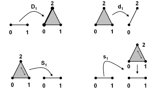
(graphics taken from Friedman 08)
Definition
For and the th degenerate -simplex (projection) is the surjective map
induced under the barycentric coordinates of def. under the surjection
which sends
Definition
For Top and , a singular -simplex in is a continuous map
from the topological -simplex, def. , to .
Write
for the set of singular -simplices of .
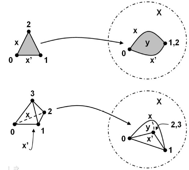
(graphics taken from Friedman 08)
The sets here are closely related by an interlocking system of maps that make them form what is called a simplicial set, and as such the collection of these sets of singular simplices is called the singular simplicial complex of . We discuss the definition of simplicial sets now and then come back to this below in def. .
Since the topological -simplices from def. sit inside each other by the face inclusions of def.
and project onto each other by the degeneracy maps, def.
we dually have functions
that send each singular -simplex to its -face and functions
that regard an -simplex as beign a degenerate (“thin”) -simplex. All these sets of simplices and face and degeneracy maps between them form the following structure.
Definition
A simplicial set is
-
for each injective map of totally ordered sets
a function – the th face map on -simplices;
-
for each surjective map of totally ordered sets
a function – the th degeneracy map on -simplices;
such that these functions satisfy the following identities, called the_simplicial identities:
-
if ,
-
if .
For two simplicial sets, a morphism of simplicial sets is for each a function between sets of -simplices, such that these functions are compatible with all the face and degeneracy maps.
This defines a category (Def. ) sSet of simplicial sets.
It is straightforward to check by explicit inspection that the evident injection and restriction maps between the sets of singular simplices make into a simplicial set. However for working with this, it is good to streamline a little:
Definition
The simplex category is the full subcategory of Cat on the free categories of the form
Remark
This is called the “simplex category” because we are to think of the object as being the “spine” of the -simplex. For instance for we think of as the “spine” of the triangle. This becomes clear if we don’t just draw the morphisms that generate the category , but draw also all their composites. For instance for we have_
Proposition
(simplicial sets are presheaves on the simplex category)
A functor
from the opposite category (Example ) of the simplex category (Def. ) to the category of sets, hence a presheaf on (Example ), is canonically identified with a simplicial set, def. .
Via this identification, the category sSet of simplicial sets (Def. ) is equivalent to the category of presheaves on the simplex category
In particular this means that sSet is a cosmos for enriched category theory (Example ), by Prop. .
Proof
One checks by inspection that the simplicial identities characterize precisely the behaviour of the morphisms in and .
This makes the following evident:
Example
The topological simplices from def. arrange into a cosimplicial object in Top, namely a functor
With this now the structure of a simplicial set on , def. , is manifest: it is just the nerve of with respect to , namely:
Definition
For a topological space its simplicial set of singular simplicies (often called the singular simplicial complex)
is given by composition of the functor from example with the hom functor of Top:
Remark
It turns out – this is the content of the homotopy hypothesis-theorem (Quillen 67) – that homotopy type of the topological space is entirely captured by its singular simplicial complex . Moreover, the geometric realization of is a model for the same homotopy type as that of , but with the special property that it is canonically a cell complex – a CW-complex. Better yet, is itself already good cell complex, namely a Kan complex. We come to this below.
Simplicial homotopy
The concept of homotopy of morphisms between simplicial sets proceeds in direct analogy with that in topological spaces.
Definition
For a simplicial set, def. , its simplicial cylinder object is the Cartesian product (formed in the category sSet, Prop. ).
between two morphisms
of simplicial sets is a morphism
such that the following diagram commutes
For a Kan complex, def. , its simplicial path space object is the function complex (formed in the category sSet, Prop. ).
between two morphisms
of simplicial sets is a morphism
such that the following diagram commutes
Proposition
For a Kan complex, def. , and any simplicial set, then left homotopy, def. , regarded as a relation
on the hom set , is an equivalence relation.
Definition
(homotopy equivalence in simplicial sets)
A morphism of simplicial sets is a left/right homotopy equivalence if there exists a morphisms and left/right homotopies (def. )
The the basic invariants of simplicial sets/Kan complexes in simplicial homotopy theory are their simplicial homotopy groups, to which we turn now.
Given that a Kan complex is a special simplicial set that behaves like a combinatorial model for a topological space, the simplicial homotopy groups of a Kan complex are accordingly the combinatorial analog of the homotopy groups of topological spaces: instead of being maps from topological spheres modulo maps from topological disks, they are maps from the boundary of a simplex modulo those from the simplex itself.
Accordingly, the definition of the discussion of simplicial homotopy groups is essentially literally the same as that of homotopy groups of topological spaces. One technical difference is for instance that the definition of the group structure is slightly more non-immediate for simplicial homotopy groups than for topological homotopy groups (see below).
Definition
For a Kan complex, then its 0th simplicial homotopy group (or set of connected components) is the set of equivalence classes of vertices modulo the equivalence relation
For a vertex and for , , then the underlying set of the th simplicial homotopy group of at – denoted – is, the set of equivalence classes of morphisms
from the simplicial -simplex to , such that these take the boundary of the simplex to , i.e. such that they fit into a commuting diagram in sSet of the form
where two such maps are taken to be equivalent is they are related by a simplicial homotopy
that fixes the boundary in that it fits into a commuting diagram in sSet of the form
These sets are taken to be equipped with the following group structure.
Definition
For a Kan complex, for , for and for two representatives of as in def. , consider the following -simplices in :
This corresponds to a morphism from a horn of the -simplex into . By the Kan complex property of this morphism has an extension through the -simplex
From the simplicial identities one finds that the boundary of the -simplex arising as the th boundary piece of is constant on
So represents an element in and we define a product operation on by
(e.g. Goerss-Jardine 99, p. 26)
Remark
All the degenerate -simplices in def. are just there so that the gluing of the two -cells and to each other can be regarded as forming the boundary of an -simplex except for one face. By the Kan extension property that missing face exists, namely . This is a choice of gluing composite of with .
Lemma
The product on homotopy group elements in def. is well defined, in that it is independent of the choice of representatives , and of the extension .
e.g. (Goerss-Jardine 99, lemma 7.1)
e.g. (Goerss-Jardine 99, theorem 7.2)
Remark
The first homotopy group, , is also called the fundamental group of .
Definition
(weak homotopy equivalence of simplicial sets)
For two Kan complexes, then a morphism
is called a weak homotopy equivalence if it induces isomorphisms on all simplicial homotopy groups, i.e. if
-
is a bijection of sets;
-
is an isomorphism of groups for all and all ; .
Kan complexes
Recall the definition of simplicial sets from above. Let
be the standard simplicial -simplex in SimpSet.
Definition
For each , , the -horn or -box is the subsimplicial set
which is the union of all faces except the one.
This is called an outer horn if or . Otherwise it is an inner horn.
Remark
Since sSet is a presheaf topos, unions of subobjects make sense and they are calculated objectwise, thus in this case dimensionwise. This way it becomes clear what the structure of a horn as a functor must therefore be: it takes to the collection of ordinal maps which do not have the element in the image.
Example
The inner horn, def. of the 2-simplex
with boundary
looks like
The two outer horns look like
and
respectively.
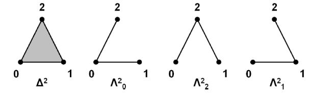
(graphics taken from Friedman 08)
Definition
A Kan complex is a simplicial set that satisfies the Kan condition,
-
which says that all horns of the simplicial set have fillers/extend to simplices;
-
which means equivalently that the unique homomorphism from to the point (the terminal simplicial set) is a Kan fibration;
-
which means equivalently that for all diagrams in sSet of the form
there exists a diagonal morphism
completing this to a commuting diagram;
-
which in turn means equivalently that the map from -simplices to -horns is an epimorphism
Proposition
For a topological space, its singular simplicial complex , def. , is a Kan complex, def. .
Proof
The inclusions of topological horns into topological simplices are retracts, in that there are continuous maps given by “squashing” a topological -simplex onto parts of its boundary, such that
Therefore the map is an epimorphism, since it is equal to to which has a right inverse .
More generally:
Definition
A morphism in sSet is called a Kan fibration if it has the right lifting property again all horn inclusions, def. , hence if for every commuting diagram of the form
there exists a lift
This is the simplicial incarnation of the concept of Serre fibrations of topological spaces:
Definition
A continuous function between topological spaces is a Serre fibration if for all CW-complexes and for every commuting diagram in Top of the form
there exists a lift
Proposition
A continuous function is a Serre fibration, def. , precisely if (def. ) is a Kan fibration, def. .
The proof uses the basic tool of nerve and realization-adjunction to which we get to below in prop. .
Proof
First observe that the left lifting property against all for a CW-complex is equivalent to left lifting against geometric realization of horn inclusions. Then apply the natural isomorphism , given by the adjunction of prop. and example , to the lifting diagrams.
Lemma
Let be a Kan fibration, def. , and let be two morphisms. If there is a left homotopy (def. ) between these maps, then there is a fiberwise homotopy equivalence, def. , between the pullback fibrations .
(e.g. Goerss-Jardine 99, chapter I, lemma 10.6)
While simplicial sets have the advantage of being purely combinatorial structures, the singular simplicial complex of any given topological space, def. is in general a huge simplicial set which does not lend itself to detailed inspection. The following is about small models.
Definition
A Kan fibration , def. , is called a minimal Kan fibration if for any two cells in the same fiber with the same boundary if they are homotopic relative their boundary, then they are already equal.
More formally, is minimal precisely if for every commuting diagram of the form
then the two composites
are equal.
Proposition
The pullback (in sSet) of a minimal Kan fibration, def. , along any morphism is again a mimimal Kan fibration.
(Goerss-Jardine 99, chapter I, section 4, Joyal-Tierney 05, section 31)
Proposition
For every Kan fibration, def. , there exists a fiberwise strong deformation retract to a minimal Kan fibration, def. .
(e.g. Goerss-Jardine 99, chapter I, prop. 10.3, Joyal-Tierney 05, theorem 3.3.1, theorem 3.3.3).
Proof idea
Choose representatives by induction, use that in the induction step one needs lifts of anodyne extensions against a Kan fibration, which exist.
Lemma
A morphism between minimal Kan fibrations, def. , which is fiberwise a homotopy equivalence, def. , is already an isomorphism.
(e.g. Goerss-Jardine 99, chapter I, lemma 10.4)
Proof idea
Show the statement degreewise. In the induction one needs to lift anodyne extensions agains a Kan fibration.
Lemma
Every minimal Kan fibration, def. , over a connected base is a simplicial fiber bundle, locally trivial over every simplex of the base.
(e.g. Goerss-Jardine 99, chapter I, corollary 10.8)
Proof
By assumption of the base being connected, the classifying maps for the fibers over any two vertices are connected by a zig-zag of homotopies, hence by lemma the fibers are connected by homotopy equivalences and then by prop. and lemma they are already isomorphic. Write for this typical fiber.
Moreover, for all the morphisms are left homotopic to and so applying lemma and prop. once more yields that the fiber over each is isomorphic to .
Groupoids as Kan complexes
Definition
-
a pair of sets (the set of objects) and (the set of morphisms)
-
equipped with functions
where the fiber product on the left is that over ,
such that
-
takes values in endomorphisms;
-
defines a partial composition operation which is associative and unital for the identities; in particular
and ;
-
every morphism has an inverse under this composition.
Remark
This data is visualized as follows. The set of morphisms is
and the set of pairs of composable morphisms is
The functions are those which send, respectively, these triangular diagrams to the left morphism, or the right morphism, or the bottom morphism.
Example
For a set, it becomes a groupoid by taking to be the set of objects and adding only precisely the identity morphism from each object to itself
Example
For a group, its delooping groupoid has
-
;
-
.
For and two groups, group homomorphisms are in natural bijection with groupoid homomorphisms
In particular a group character is equivalently a groupoid homomorphism
Here, for the time being, all groups are discrete groups. Since the circle group also has a standard structure of a Lie group, and since later for the discussion of Chern-Simons type theories this will be relevant, we will write from now on
to mean explicitly the discrete group underlying the circle group. (Here “” denotes the “flat modality”.)
Example
For a set, a discrete group and an action of on (a permutation representation), the action groupoid or homotopy quotient of by is the groupoid
with composition induced by the product in . Hence this is the groupoid whose objects are the elements of , and where morphisms are of the form
for , .
As an important special case we have:
Example
For a discrete group and the trivial action of on the point (the singleton set), the corresponding action groupoid according to def. is the delooping groupoid of according to def. :
Another canonical action is the action of on itself by right multiplication. The corresponding action groupoid we write
The constant map induces a canonical morphism
This is known as the -universal principal bundle. See below in for more on this.
Example
For a topological space, its fundamental groupoid is
- points in ;
- continuous paths in modulo homotopy that leaves the endpoints fixed.
Example
For any groupoid, there is the path space groupoid with
-
;
-
commuting squares in =
This comes with two canonical homomorphisms
which are given by endpoint evaluation, hence which send such a commuting square to either its top or its bottom hirizontal component.
Definition
For two morphisms between groupoids, a homotopy (a natural transformation) is a homomorphism of the form (with codomain the path space object of as in example ) such that it fits into the diagram as depicted here on the right:
Definition (Notation)
Here and in the following, the convention is that we write
-
(with the subscript decoration) when we regard groupoids with just homomorphisms (functors) between them,
-
(without the subscript decoration) when we regard groupoids with homomorphisms (functors) between them and homotopies (natural transformations) between these
The unbulleted version of groupoids are also called homotopy 1-types (or often just their homotopy-equivalence classes are called this way.) Below we generalize this to arbitrary homotopy types (def. ).
Definition
A (homotopy-) equivalence of groupoids is a morphism which has a left and right inverse up to homotopy.
Example
The map
which picks any point and sends to the loop based at that point which winds around times, is an equivalence of groupoids.
Proposition
Assuming the axiom of choice in the ambient set theory, every groupoid is equivalent to a disjoint union of delooping groupoids, example – a skeleton.
Remark
The statement of prop. becomes false as when we pass to groupoids that are equipped with geometric structure. This is the reason why for discrete geometry all Chern-Simons-type field theories (namely Dijkgraaf-Witten theory-type theories) fundamentally involve just groups (and higher groups), while for nontrivial geometry there are genuine groupoid theories, for instance the AKSZ sigma-models. But even so, Dijkgraaf-Witten theory is usefully discussed in terms of groupoid technology, in particular since the choice of equivalence in prop. is not canonical.
Definition
Given two morphisms of groupoids their homotopy fiber product
hence the ordinary iterated fiber product over the path space groupoid, as indicated.
Remark
An ordinary fiber product of groupoids is given simply by the fiber product of the underlying sets of objects and morphisms:
Example
For a groupoid, a group and a map into its delooping, the pullback of the -universal principal bundle of example is equivalently the homotopy fiber product of with the point over :
Namely both squares in the following diagram are pullback squares
(This is the first example of the more general phenomenon of universal principal infinity-bundles.)
Example
For a groupoid and a point in it, we call
the loop space groupoid of .
For a group and its delooping groupoid from example , we have
Hence is the loop space object of its own delooping, as it should be.
Proof
We are to compute the ordinary limiting cone in
In the middle we have the groupoid whose objects are elements of and whose morphisms starting at some element are labeled by pairs of elements and end at . Using remark the limiting cone is seen to precisely pick those morphisms in such that these two elements are constant on the neutral element , hence it produces just the elements of regarded as a groupoid with only identity morphisms, as in example .
Proposition
The free loop space object is
Proof
Notice that . Therefore the path space object has
-
objects are pairs of morphisms in ;
-
morphisms are commuting squares of such.
Now the fiber product in def. picks in there those pairs of morphisms for which both start at the same object, and both end at the same object. Therefore is the groupoid whose
-
objects are diagrams in of the form
-
morphism are cylinder-diagrams over these.
One finds along the lines of example that this is equivalent to maps from into and homotopies between these.
Remark
Even though all these models of the circle are equivalent, below the special appearance of the circle in the proof of prop. as the combination of two semi-circles will be important for the following proofs. As we see in a moment, this is the natural way in which the circle appears as the composition of an evaluation map with a coevaluation map.
Example
For a discrete group, the free loop space object of its delooping is , the action groupoid, def. , of the adjoint action of on itself:
Example
For an abelian group such as we have
Example
Let be a group homomorphism, hence a group character. By example this has a delooping to a groupoid homomorphism
Under the free loop space object construction this becomes
hence
So by postcomposing with the projection on the first factor we recover from the general homotopy theory of groupoids the statement that a group character is a class function on conjugacy classes:
Definition
For a groupoid, def. , its simplicial nerve is the simplicial set with
the set of sequences of composable morphisms of length , for ;
with face maps
being,
-
for the functions that remembers the th object;
-
for
-
the two outer face maps and are given by forgetting the first and the last morphism in such a sequence, respectively;
-
the inner face maps are given by composing the th morphism with the st in the sequence.
-
The degeneracy maps
are given by inserting an identity morphism on .
Remark
Spelling this out in more detail: write
for the set of sequences of composable morphisms. Given any element of this set and , write
for the comosition of the two morphism that share the th vertex.
With this, face map acts simply by “removing the index ”:
Similarly, writing
for the identity morphism on the object , then the degenarcy map acts by “repeating the th index”
This makes it manifest that these functions organise into a simplicial set.
Proposition
These collections of maps in def. satisfy the simplicial identities, hence make the nerve into a simplicial set. Moreover, this simplicial set is a Kan complex, where each horn has a unique filler (extension to a simplex).
(A 2-coskeletal Kan complex.)
Proposition
The nerve operation constitutes a full and faithful functor
Chain complexes as Kan complexes
In the familiar construction of singular homology recalled above one constructs the alternating face map chain complex of the simplicial abelian group of singular simplices, def. . This construction is natural and straightforward, but the result chain complex tends to be very “large” even if its chain homology groups end up being very “small”. But in the context of homotopy theory one is to consider all objects notup to isomorphism, but of to weak equivalence, which for chain complexes means up to quasi-isomorphisms. Hence one should look for the natural construction of “smaller” chain complexes that are still quasi-isomorphic to these alternating face map complexes. This is accomplished by the normalized chain complex construction:
Definition
For a simplicial abelian group its alternating face map complex of is the chain complex which
-
in degree is given by the group itself
-
with differential given by the alternating sum of face maps (using the abelian group structure on )
Proof
Using the simplicial identity, prop. , for one finds:
Definition
Given a simplicial abelian group , its normalized chain complex or Moore complex is the -graded chain complex which
-
is in degree the joint kernel
of all face maps except the 0-face;
-
with differential given by the remaining 0-face map
Remark
We may think of the elements of the complex , def. , in degree as being -dimensional disks in all whose boundary is captured by a single face:
-
an element in degree 1 is a 1-disk
-
an element is a 2-disk
-
a degree 2 element in the kernel of the boundary map is such a 2-disk that is closed to a 2-sphere
etc.
Definition
Given a simplicial group (or in fact any simplicial set), then an element is called degenerate (or thin) if it is in the image of one of the simplicial degeneracy maps . All elements of are regarded a non-degenerate. Write
for the subgroup of which is generated by the degenerate elements (i.e. the smallest subgroup containing all the degenerate elements).
Definition
For a simplicial abelian group its alternating face maps chain complex modulo degeneracies, is the chain complex
-
which in degree 0 equals is just ;
-
which in degree is the quotient group obtained by dividing out the group of degenerate elements, def. :
-
whose differential is the induced action of the alternating sum of faces on the quotient (which is well-defined by lemma ).
Lemma
Def. is indeed well defined in that the alternating face map differential respects the degenerate subcomplex.
Proof
Using the mixed simplicial identities we find that for a degenerate element, its boundary is
which is again a combination of elements in the image of the degeneracy maps.
Proposition
Given a simplicial abelian group , the evident composite of natural morphisms
from the normalized chain complex, def. , into the alternating face map complex modulo degeneracies, def. , (inclusion followed by projection to the quotient) is a natural isomorphism of chain complexes.
e.g. (Goerss-Jardine, theorem III 2.1).
Corollary
For a simplicial abelian group, there is a splitting
of the alternating face map complex, def. as a direct sum, where the first direct summand is naturally isomorphic to the normalized chain complex of def. and the second is the degenerate cells from def. .
Proof
By prop. there is an inverse to the diagonal composite in
This hence exhibits a splitting of the short exact sequence given by the quotient by .
Theorem
(Eilenberg-MacLane)
Given a simplicial abelian group , then the inclusion
of the normalized chain complex, def. into the full alternating face map complex, def. , is a natural quasi-isomorphism and in fact a natural chain homotopy equivalence, i.e. the complex is null-homotopic.
(Goerss & Jardine, theorem III 2.4)
Corollary
Given a simplicial abelian group , then the projection chain map
from its alternating face maps complex, def. , to the alternating face map complex modulo degeneracies, def. , is a quasi-isomorphism.
Proof
Consider the pre-composition of the map with the inclusion of the normalized chain complex, def. .
By theorem the vertical map is a quasi-isomorphism and by prop. the composite diagonal map is an isomorphism, hence in particular also a quasi-isomorphism. Since quasi-isomorphisms satisfy the two-out-of-three property, it follows that also the map in question is a quasi-isomorphism.
Example
Consider the 1-simplex regarded as a simplicial set, and write for the simplicial abelian group which in each degree is the free abelian group on the simplices in .
This simplicial abelian group starts out as
(where we are indicating only the face maps for notational simplicity).
Here the first , the direct sum of two copies of the integers, is the group of 0-chains generated from the two endpoints and of , i.e. the abelian group of formal linear combinations of the form
The second is the abelian group generated from the three (!) 1-simplicies in , namely the non-degenerate edge and the two degenerate cells and , hence the abelian group of formal linear combinations of the form
The two face maps act on the basis 1-cells as
Now of course most of the (infinitely!) many simplices inside are degenerate. In fact the only non-degenerate simplices are the two 0-cells and and the 1-cell . Hence the alternating face maps complex modulo degeneracies, def. , of is simply this:
Notice that alternatively we could consider the topological 1-simplex and its singular simplicial complex in place of the smaller , then the free simplicial abelian group of that. The corresponding alternating face map chain complex is “huge” in that in each positive degree it has a free abelian group on uncountably many generators. Quotienting out the degenerate cells still leaves uncountably many generators in each positive degree (while every singular -simplex in is “thin”, only those whose parameterization is as induced by a degeneracy map are actually regarded as degenerate cells here). Hence even after normalization the singular simplicial chain complex is “huge”. Nevertheless it is quasi-isomorphic to the tiny chain complex found above.
The statement of the Dold-Kan correspondence now is the following.
Theorem
For an abelian category there is an equivalence of categories
between
-
the category of simplicial objects in ;
where
- is the normalized chains complex/normalized Moore complex functor.
(Dold 58, Kan 58, Dold-Puppe 61).
Theorem
For the case that is the category Ab of abelian groups, the functors and are nerve and realization with respect to the cosimplicial chain complex
that sends the standard -simplex to the normalized Moore complex of the free simplicial abelian group on the simplicial set , i.e.
This is due to (Kan 58).
More explicitly we have the following
Proposition
-
For the simplicial abelian group is in degree given by
and for a morphism in the corresponding map
is given on the summand indexed by some by the composite
where
is the epi-mono factorization of the composite .
-
The natural isomorphism is given on by the map
which on the direct summand indexed by is the composite
-
The natural isomorphism is on a chain complex given by the composite of the projection
with the inverse
of
(which is indeed an isomorphism, as discussed at Moore complex).
This is spelled out in (Goerss-Jardine, prop. 2.2 in section III.2).
Proposition
With the explicit choice for as above we have that and form an adjoint equivalence
This is for instance (Weibel, exercise 8.4.2).
Remark
It follows that with the inverse structure maps, we also have an adjunction the other way round: .
Hence in conclusion the Dold-Kan correspondence allows us to regard chain complexes (in non-negative degree) as, in particular, special simplicial sets. In fact as simplicial sets they are Kan complexes and hence infinity-groupoids:
Theorem
The simplicial set underlying any simplicial group (by forgetting the group structure) is a Kan complex.
This is due to (Moore, 1954)
In fact, not only are the horn fillers guaranteed to exist, but there is an algorithm that provides explicit fillers. This implies that constructions on a simplicial group that use fillers of horns can often be adjusted to be functorial by using the algorithmically defined fillers. An argument that just uses ‘existence’ of fillers can be refined to give something more ‘coherent’.
Proof
Let be a simplicial group.
Here is the explicit algorithm that computes the horn fillers:
Let give a horn in , so the s are simplices that fit together as if they were all but one, the one, of the faces of an -simplex. There are three cases:
-
if :
- Let and then for , then satisfies , ;
-
if :
- Let and for , then take , and finally a downwards induction given by , for , then gives for ;
-
if :
- use and for , then satisfies , .
Geometric realization
So far we we have considered passing from topological spaces to simplicial sets by applying the singular simplicial complex functor of def. . Now we discuss a left adjoint of this functor, called geometric realization, which turns a simplicial set into a topological space by identifying each of its abstract n-simplices with the standard topological -simplex.
This is an example of a general abstract phenomenon:
Proposition
Let
be a functor from a small category to a locally small category with all colimits. Then the nerve-functor
has a left adjoint functor , called geometric realization,
given by the coend
(Kan 58)
Example
The singular simplicial complex functor of def. has a left adjoint geometric realization functor
given by the coend
Topological geometric realization takes values in particularly nice topological spaces.
Proposition
The topological geometric realization of simplicial sets in example takes values in CW-complexes.
(e.g. Goerss-Jardine 99, chapter I, prop. 2.3)
Thus for a topological space the adjunction counit of the nerve and realization-adjunction is a candidate for a replacement of by a CW-complex. For this, should be at least a weak homotopy equivalence, i.e. induce isomorphisms on all homotopy groups. Since homotopy groups are built from maps into out of compact topological spaces it is plausible that this works if the topology of is entirely detected by maps out of compact topological spaces into . Topological spaces with this property are called compactly generated.
We take compact topological space to imply Hausdorff topological space.
Definition
A subspace of a topological space is called compactly open or compactly closed, respectively, if for every continuous function out of a compact topological space the preimage is open or closed, respectively.
A topological space is a compactly generated topological space if each of its compactly closed subspaces is already closed.
Write
for the full subcategory of Top on the compactly generated topological spaces.
Often the condition is added that a compactly closed topological space be also a weakly Hausdorff topological space.
Example
Examples of compactly generated topological spaces, def. , include
-
every compact space;
-
every locally compact space;
-
every topological manifold;
-
every CW-complex;
-
every first countable space
Corollary
The topological geometric realization functor of simplicial sets in example takes values in compactly generated topological spaces
Proposition
The subcategory of def. has the following properties
-
It is a coreflective subcategory
The coreflection of a topological space is given by adding to the open subsets of all compactly open subsets, def. .
-
It has all small limits and colimits.
The colimits are computed in , the limits are the image under of the limits as computed in .
-
It is a cartesian closed category.
The cartesian product in is the image under of the Cartesian product formed in .
This is due to (Steenrod 67), expanded on in (Lewis 78, appendix A). One says that prop. with example makes a “convenient category of topological spaces”.
Proposition
Regarded, via corollary as a functor , geometric realization preserves finite limits.
See at Geometric realization is left exact.
Proof idea
The key step in the proof is to use the cartesian closure of (prop. ). This gives that the Cartesian product is a left adjoint and hence preserves colimits in each variable, so that the coend in the definition of the geometric realization may be taken out of Cartesian products.
Lemma
The geometric realization, example , of a minimal Kan fibration, def. is a Serre fibration, def. .
This is due to (Gabriel-Zisman 67). See for instance (Goerss-Jardine 99, chapter I, corollary 10.8, theorem 10.9).
Proof idea
By prop. minimal Kan fibrations are simplicial fiber bundles, locally trivial over each simplex in the base. By prop. this property translates to their geometric realization also being a locally trivial fiber bundle of topological spaces, hence in particular a Serre fibration.
Proposition
The geometric realization, example , of any Kan fibration, def. is a Serre fibration, def. .
This is due to (Quillen 68). See for instance (Goerss-Jardine 99, chapter I, theorem 10.10).
Proposition
For a Kan complex, then the unit of the nerve and realization-adjunction (prop. , example )
is a weak homotopy equivalence, def. .
For any topological space, then the adjunction counit
e.g. (Goerss-Jardine 99, chapter I, prop. 11.1 and p. 63).
Proof idea
Use prop. and prop. applied to the path fibration to proceed by induction.
The classical model structure on simplicial sets
Definition
(classical model structure on simplicial sets)
The classical model structure on simplicial sets, , has the following distinguished classes of morphisms:
-
The classical weak equivalences are the morphisms whose geometric realization, example , is a weak homotopy equivalence of topological spaces;
-
The classical fibrations are the Kan fibrations, def. ;
-
The classical cofibrations are the monomorphisms of simplicial sets, i.e. the degreewise injections.
Proposition
In model structure , def. , the following holds.
-
The fibrant objects are precisely the Kan complexes.
-
A morphism of fibrant simplicial sets / Kan complexes is a weak equivalence precisely if it induces an isomorphism on all simplicial homotopy groups, def. .
-
All simplicial sets are cofibrant with respect to this model structure.
Proposition
The acyclic fibrations in (i.e. the maps that are both fibrations as well as weak equivalences) between Kan complexes are precisely the morphisms that have the right lifting property with respect to all inclusions of boundaries of -simplices into their -simplices
This appears spelled out for instance as (Goerss-Jardine 99, theorem 11.2).
In fact:
Proposition
is a cofibrantly generated model category with
Theorem
Let be the smallest class of morphisms in satisfying the following conditions:
- The class of monomorphisms that are in is closed under pushout, transfinite composition, and retracts.
- has the two-out-of-three property in and contains all the isomorphisms.
- For all natural numbers , the unique morphism is in .
Then is the class of weak homotopy equivalences.
Proof
- First, notice that the horn inclusions and are in .
- Suppose that the horn inclusion is in for all and all . Then for , the horn inclusion is also in .
- Quillen’s small object argument then implies all the trivial cofibrations are in .
- If is a trivial Kan fibration, then its right lifting property implies there is a morphism such that , and the two-out-of-three property implies is a trivial cofibration. Thus every trivial Kan fibration is also in .
- Every weak homotopy equivalence factors as where is a trivial Kan fibration and is a trivial cofibration, so every weak homotopy equivalence is indeed in .
- Finally, noting that the class of weak homotopy equivalences satisfies the conditions in the theorem, we deduce that it is the smallest such class.
As a corollary, we deduce that the classical model structure on is the smallest (in terms of weak equivalences) model structure for which the cofibrations are the monomorphisms and the weak equivalences include the (combinatorial) homotopy equivalences.
Proposition
Let be the connected components functor, i.e. the left adjoint of the constant functor . A morphism in is a weak homotopy equivalence if and only if the induced map
is a bijection for all Kan complexes .
Proof
One direction is easy: if is a Kan complex, then axiomS FOR simplicial model categories (Def. ) implies the functor is a right Quillen functor, so Ken Brown's lemma (Prop. ) implies that it preserves all weak homotopy equivalences; in particular, sends weak homotopy equivalences to bijections.
Conversely, when is a Kan complex, there is a natural bijection between and the hom-set , and thus by the Yoneda lemma, a morphism such that the induced morphism is a bijection for all Kan complexes is precisely a morphism that becomes an isomorphism in , i.e. a weak homotopy equivalence.
Theorem
(Quillen equivalence between classical model structure on topological spaces and classical model structure on simplicial sets)
The singular simplicial complex/geometric realization-adjunction of example constitutes a Quillen equivalence between the classical model structure on simplicial sets of def. and the classical model structure on topological spaces:
Proof
First of all, the adjunction is indeed a Quillen adjunction: prop. says in particular that takes Serre fibrations to Kan fibrations and prop. gives that sends monomorphisms of simplicial sets to relative cell complexes.
Now prop. says that the derived adjunction unit and derived adjunction counit are weak equivalences, and hence the Quillen adjunction is a Quillen equivalence.
Last revised on November 22, 2025 at 08:39:24. See the history of this page for a list of all contributions to it.