nLab Introduction to Topology -- 2
This page (cf. pdf, 61p) is an introduction to basic topological homotopy theory. We introduce the concept of homotopy between continuous functions and the induced concept of homotopy equivalence of topological spaces. Homotopy classes of paths form the fundamental groupoid of a topological space, the first step in extracting combinatorial data in homotopy theory. We use this example to introduce groupoids and their homotopy theory in general and mention that this models the homotopy theory of those topological spaces that are homotopy 1-types. Then we discuss the concept of covering spaces and use groupoids to give a simple proof of the fundamental theorem of covering spaces, which says that these are equivalent to permutation representations of the fundamental groupoid. This is a simple topological version of the general principle of Galois theory and has many applications. As one example application, we use it to prove that the fundamental group of the circle is the integers.
main page: Introduction to Topology
previous chapter: Introduction to Topology 1 – Point-set topology
this chapter: Introduction to Topology 2 – Basic Homotopy Theory
For introduction to more general and abstract homotopy theory see instead at Introduction to Homotopy Theory.
Context
Topology
topology (point-set topology, point-free topology)
see also differential topology, algebraic topology, functional analysis and topological homotopy theory
Basic concepts
-
fiber space, space attachment
Extra stuff, structure, properties
-
Kolmogorov space, Hausdorff space, regular space, normal space
-
sequentially compact, countably compact, locally compact, sigma-compact, paracompact, countably paracompact, strongly compact
Examples
Basic statements
-
closed subspaces of compact Hausdorff spaces are equivalently compact subspaces
-
open subspaces of compact Hausdorff spaces are locally compact
-
compact spaces equivalently have converging subnet of every net
-
continuous metric space valued function on compact metric space is uniformly continuous
-
paracompact Hausdorff spaces equivalently admit subordinate partitions of unity
-
injective proper maps to locally compact spaces are equivalently the closed embeddings
-
locally compact and second-countable spaces are sigma-compact
Theorems
Analysis Theorems
Homotopy theory
homotopy theory, (∞,1)-category theory, homotopy type theory
flavors: stable, equivariant, rational, p-adic, proper, geometric, cohesive, directed…
models: topological, simplicial, localic, …
see also algebraic topology
Introductions
Definitions
Paths and cylinders
Homotopy groups
Basic facts
Theorems
Basic Homotopy Theory
In order to handle topological spaces, to compute their properties and to distinguish them, it turns out to be useful to consider not just continuous variation within a topological space, i.e. continuous functions between topological spaces, but also continuous deformations of continuous functions themselves. This is the concept of homotopy (def. below), and its study is called homotopy theory. If one regards topological spaces with homotopy classes of continuous functions between them then their nature changes, and one speaks of homotopy types (remark below).
Of particular interest are homotopies between paths in a topological space. If a loop in a topological space is homotopic to the constant loop, this means that it does not “wind around a hole” in the space. Hence the set of homotopy classes of loops in a topological space, which is a group under concatenation of paths, detects crucial information about the global structure of the space, and hence is called the fundamental group of the space (def. ).
This same information turns out to be encoded in “continuously varying sets” over a topological space, hence in “bundles of sets”, called covering spaces (def. below). As one moves around a loop, then the parameterized set comes back to itself up to a bijection called the monodromy of the loop. This encodes an action or permutation representation of the fundamental group. The fundamental theorem of covering spaces (prop. below) says that covering spaces are equivalently characterized by their monodromy representation of the fundamental group. This is an incarnation of the general principle of Galois theory in topological homotopy theory. Sometimes this allows to compute fundamental groups from behaviour of covering spaces, for instance it allows to prove that the fundamental group of the circle is the integers (prop. below).
In order to formulate and prove these statements, it turns out convenient to do away with the arbitrary choice of basepoint that is involved in the definition of fundamental groups, and instead collect all homotopy classes of paths into a single structure, called the fundamental groupoid of a topological space (example below) an example of a generalization of groups to groupoids (discussed below). The fundamental groupoid may be regarded as an algebraic incarnation of the homotopy type presented by a topological space, up to level 1 (the homotopy 1-type).
The algebraic reflection of the full homotopy type of a topological space involves higher dimensional analogs for the fundamental group called the higher homotopy groups. We close with an outlook on these below.
Homotopy
It is clear that for the Euclidean space or equivalently the open ball in is not homeomorphic to the point space (simply because there is not even a bijection between the underlying sets). Nevertheless, intuitively the -ball is a “continuous deformation” of the point, obtained as the radius of the -ball tends to zero.
This intuition is made precise by observing that there is a continuous function out of the product topological space (this example) of the open ball with the closed interval
which is given by rescaling:
This continuously interpolates between the open ball and the point, in that for it restricts to the identity, while for it restricts to the map constant on the origin.
We may summarize this situation by saying that there is a diagram of continuous functions of the form
Such “continuous deformations” are called homotopies:
In the following we use this terminology:
Definition
The topological interval is
-
the closed interval regarded as a topological space in the standard way, as a subspace of the real line with its Euclidean metric topology,
-
equipped with the continuous functions
which include the point space as the two endpoints, respectively
-
equipped with the (unique) continuous function
to the point space (which is the terminal object in Top)
regarded, in summary, as a factorization
of the codiagonal on the point space, namely the unique continuous function out of the disjoint union space (homeomorphic to the discrete topological space on two elements).
Definition
(homotopy)
Let Top be two topological spaces and let
be two continuous functions between them.
A (left) homotopy from to , to be denoted
is a continuous function
out of the product topological space (this example) of the topological interval (def. ) such that this makes the following diagram in Top commute:
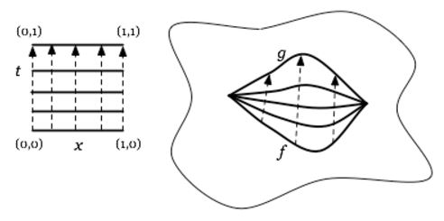
graphics grabbed from J. Tauber here
hence such that
If there is a homotopy (possibly unspecified) we say that is homotopic to , denoted
Proposition
(homotopy is an equivalence relation)
Let Top be two topological spaces. Write for the set of continuous functions from to .
Then the relating of being homotopic (def. ) is an equivalence relation on this set. The corresponding quotient set
is called the set of homotopy classes of continuous functions.
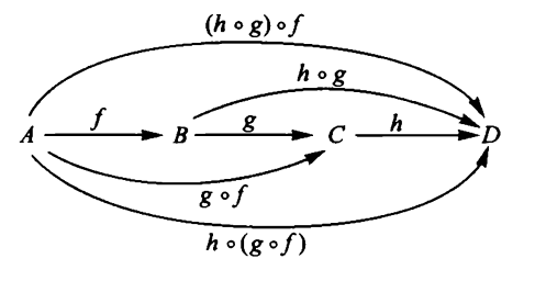
Moreover, this equivalence relation is compatible with composition of continuous functions:
For Top three topological spaces, there is a unique function
such that the following diagram commutes:
Proof
To see that the relation is reflexive: A homotopy from a function to itself is given by the function which is constant on the topological interval:
This is continuous because projections out of product topological spaces are continuous, by the universal property of the Cartesian product.
To see that the relation is symmetric: If is a homotopy then
is a homotopy . This is continuous because is a polynomial function, and polynomials are continuous, and because Cartesian product and composition of continuous functions is again continuous.
Finally to see that the relation is transitive: If and are two composable homotopies, then consider the “-parameterized path concatenation”
To see that this is continuous, observe that is a cover of by closed subsets (in the product topology) and because and are continuous (being composites of Cartesian products of continuous functions) and agree on the intersection . Hence the continuity follows by this example.
Finally to see that homotopy respects composition: Let
be continuous functions, and let
be a homotopy. It is sufficient to show that then there is a homotopy of the form
This is exhibited by the following diagram
Remark
Prop. means that homotopy classes of continuous functions are the morphisms in a category whose objects are still the topological spaces.
This category (at least when restricted to spaces that admit the structure of CW-complexes) is called the classical homotopy category, often denoted
Hence for topological spaces, then
Moreover, sending a continuous function to its homotopy class is a functor
from the ordinary category Top of topological spaces with actual continuous functions between them.
Definition
Let Top be two topological spaces.
is called a homotopy equivalence if there exists
-
a continuous function the other way around,
-
homotopies (def. ) from the two composites to the respective identity function:
and
We indicate that a continuous function is a homotopy equivalence by writing
If there exists some (possibly unspecified) homotopy equivalence between topological spaces and we write
Remark
(homotopy equivalences are the isomorphisms in the homotopy category)
In view of remark a continuous function is a homotopy equivalence precisely if its image in the homotopy category is an isomorphism.
As an object of the homotopy category, a topological space is often referred to as a (strong) homotopy type. Homotopy types have a different nature than the topological spaces which present them, in that topological spaces that are far from being homeomorphic may still be equivalent as homotopy types.
Example
(homeomorphism is homotopy equivalence)
Every homeomorphism is a homotopy equivalence (def. ).
Proposition
(homotopy equivalence is equivalence relation)
Being homotopy equivalent is an equivalence relation on the class of topological spaces.
Proof
This is immediate from remark by general properties of categories and functors.
But for the record we spell it out. This involves the construction already used in the proof of prop. :
It is clear that the relation it reflexive and symmetric. To see that it is transitive consider continuous functions
and homotopies
We need to produce homotopies of the form
and
Now the diagram
with one of the given homotopies, exhibits a homotopy . Composing this with the given homotopy gives the first of the two homotopies required above. The second one follows by the same construction, just with the labels of the functions exchanged.
Definition
(contractible topological space)
A topological space is called contractible if the unique continuous function to the point space
is a homotopy equivalence (def. ).
Remark
(contractible topological spaces are the terminal objects in the homotopy category)
In view of remark , a topological space is contractible (def. ) precisely if its image in the classical homotopy category is a terminal object.
Example
(closed ball and Euclidean space are contractible)
Let be the unit open ball or closed ball in Euclidean space. This is contractible (def. ):
The homotopy inverse function is necessarily constant on a point, we may just as well choose it to go pick the origin:
For one way of composing these functions we have the equality
with the identity function. This is a homotopy by prop. .
The other composite is
Hence we need to produce a homotopy
This is given by the function
where on the right we use the multiplication with respect to the standard real vector space structure in .
Since the open ball is homeomorphic to the whole Cartesian space (this example) it follows with example and example that also is a contractible topological space:
In direct generalization of the construction in example one finds further examples as follows:
Example
The following three graphs
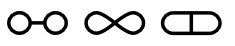
(i.e. the evident topological subspaces of the plane that these pictures indicate) are not homeomorphic. But they are homotopy equivalent, in fact they are each homotopy equivalent to the disk with two points removed, by the homotopies indicated by the following pictures:
graphics grabbed from Hatcher
Fundamental group
Definition
Let be a topological space and let
be two paths in , i.e. two continuous functions from the closed interval to , such that their endpoints agree:
Then a homotopy relative boundary from to is a homotopy (def. )
such that it does not move the endpoints:
Proposition
(homotopy relative boundary is equivalence relation on sets of paths)
Let be a topological space and let be two points. Write
for the set of paths in with and .
Then homotopy relative boundary (def. ) is an equivalence relation on .
The corresponding set of equivalence classes is denoted
Recall the operations on paths: path concatenation , path reversion and constant paths
Proposition
(concatenation of homotopy relative boundary-classes of paths)
For a topological space, then the operation of path concatenation descends to homotopy relative boundary equivalence classes, so that for all there is a function
Moreover,
-
this composition operation is associative in that for all and , and then
-
this composition operation is unital with neutral elements the constant paths in that for all and we have
-
this composition operation has inverse elements given by path reversal in that for all and we have
Definition
(fundamental groupoid and fundamental groups)
Let be a topological space. Then set of points of together with the sets of homotopy relative boundary-classes of paths (def. ) for all points of points and equipped with the concatenation operation from prop. is called the fundamental groupoid of , denoted
Given a choice of point , then one writes
Prop. says that under concatenation of paths, this set is a group. As such it is called the fundamental group of at .
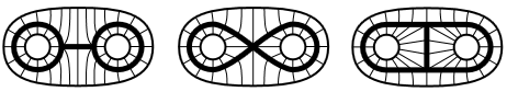
The following picture indicates the four non-equivalent non-trivial generators of the fundamental group of the oriented surface of genus 2:
graphics grabbed from Lawson 03
Example
(fundamental group of Euclidean space)
For and any point in the -dimensional Euclidean space (regarded with its metric topology) we have that the fundamental group (def. ) at that point is trivial:
Remark
(basepoints)
Definition intentionally offers two variants of the definition.
The first, the fundamental groupoid is canonically given, without choosing a basepoint. As a result, it is a structure that is not quite a group but, slightly more generally, a “groupoid” (a “group with many objects”). We discuss the concept of groupoids below.
The second, the fundamental group, is a genuine group, but its definition requires picking a base point .
In this context it is useful to say that
-
a pointed topological space is
-
a in the underlying set.
-
a homomorphism of pointed topological spaces is a base-point preserving continuous function, namely
-
such that .
Hence there is a category, to be denoted, , whose objects are the pointed topological spaces, and whose morphisms are tbe base-point preserving continuous functions.
Similarly, a homotopy between morphisms in is a homotopy of underlying continuous functions, as in def. , such that the corresponding function
preserves the basepoints in that
These pointed homotopies still form an equivalence relation as in prop. and hence quotienting these out yields the pointed analogue of the homotopy category from def. , now denoted
In general it is hard to explicitly compute the fundamental group of a topological space. But often it is already useful to know if two spaces have the same fundamental group or not:
Definition
(pushforward of elements of fundamental groups)
Let and be pointed topological space (remark ) and let
be a continuous function which respects the chosen points, in that .
Then there is an induced homomorphism of fundamental groups (def. )
given by sending a closed path to the composite
Remark
(fundamental group is functor on pointed topological spaces)
The pushforward operation in def. is functorial, now on the category of pointed topological spaces (remark )
Proposition
(fundamental group depends only on homotopy classes)
Let be pointed topological space and let be two base-point preserving continuous functions. If there is a pointed homotopy (def. , remark )
then the induced homomorphisms on fundamental groups (def. ) agree
In particular if is a homotopy equivalence (def. ) then is an isomorphism.
Proof
This follows by the fact that homotopy respects composition (prop. ):
If is a closed path representing a given element of , then the homotopy induces a homotopy
and therefore these represent the same elements in .
If follows that if is a homotopy equivalence with homotopy inverse , then is an inverse morphism to and hence is an isomorphism.
Remark
Prop. says that the fundamental group functor from def. and remark factors through the classical pointed homotopy category from remark :
Definition
(simply connected topological space)
A topological space for which
-
(the fundamental group is trivial, def. ),
is called simply connected.
We will need also the following local version:
Definition
(semi-locally simply connected topological space)
A topological space is called semi-locally simply connected if every point has a neighbourhood such that every loop in is contractible as a loop in , hence such that the induced morphism of fundamental groups (def. )
is trivial (i.e. sends everything to the neutral element).
If every has a neighbourhood which is itself simyply connected, then is called a locally simply connected topological space. This implies semi-local simply-connectedness.
Example
(Euclidean space is simply connected)
For , then the Euclidean space is a simply connected topological space (def. ).
Groupoids
In def. we extracted the fundamental group at some point from a larger algebraic structure, that incorporates all the basepoints, to be called the fundamental groupoid. This larger algebraic structure of groupoids is usefully made explicit for the formulation and proof of the fundamental theorem of covering spaces (theorem below) and the development of homotopy theory in general.
Where a group may be thought of as a group of symmetry transformations that isomorphically relates one object to itself (the symmetries of one object, such as the isometries of a polyhedron) a groupoid is a collection of symmetry transformations acting between possibly more than one object.
Hence a groupoid consists of a set of objects and for each pair of objects there is a set of transformations, usually denoted by arrows
which may be composed if they are composable (i.e. if the first ends where the second starts)
such that this composition is associative and such that for each object there is identity transformation in that this is a neutral element for the composition of transformations, whenever defined.
So far this structure is what is called a small category. What makes this a (small) groupoid is that all these transformations are to be “symmetries” in that they are invertible morphisms meaning that for each transformation there is a transformation the other way around such that
If there is only a single object , then this definition reduces to that of a group, and in this sense groupoids are “groups with many objects”. Conversely, given any groupoid and a choice of one of its objects , then the subcollection of transformations from and to is a group, sometimes called the automorphism group of in .
Just as for groups, the “transformations” above need not necessarily be given by concrete transformations (say by bijections between objects which are sets). Just as for groups, such a concrete realization is always possible, but is an extra choice (called a representation of the groupoid). Generally one calls these “transformations” morphisms: is a morphism with “source” and “domain” .
An archetypical example of a groupoid is the fundamental groupoid of a topological space (def. below, for introduction see here): For a topological space, this is the groupoid whose
-
objects are the points ;
-
morphisms are the homotopy relative boundary-equivalence classes of paths in , with and ;
and composition is given, on representatives, by concatenation of paths. Here the class of the reverse path constitutes the inverse morphism, making this a groupoid.
If one chooses a point , then the corresponding group at that point is the fundamental group of at that point.
This highlights one of the reasons for being interested in groupoids over groups: Sometimes this allows to avoid unnatural ad-hoc choices and it serves to streamline and simplify the theory.
A homomorphism between groupoids is the obvious: a function between their underlying objects together with a function between their morphisms which respects source and target objects as well as composition and identity morphisms. If one thinks of the groupoid as a special case of a category, then this is a functor. Between groupoids with only a single object this is the same as a group homomorphism.
For example if is a continuous function between topological spaces, then postcomposition of paths with this function induces a groupoid homomorphism between the fundamental groupoids from above.
Groupoids with groupoid homomorphisms (functors) between them form a category Grpd (def. below) which includes the category Grp of groups as the full subcategory of the groupoids with a single object. This makes precise how groupoid theory is a generalization of group theory.
However, for groupoids more than for groups one is typically interested in “conjugation actions” on homomorphisms. These are richer for groupoids than for groups, because one may conjugate with a different morphism at each object. If we think of groupoids as special cases of categories, then these “conjugation actions on homomorphisms” are natural transformations between functors.
For examples if are two continuous functions between topological spaces, and if is a homotopy from to , then the homotopy relative boundary classes of the paths constitute a natural transformation between in that for all paths in we have the “conjugation relation”
Definition
(groupoid)
A small groupoid is
-
for all pairs of objects a set , to be called the set of morphisms with domain or source and codomain or target ;
-
for all triples of objects a function
to be called composition
-
for all objects an element
to be called the identity morphism on ;
-
for all pairs of objects a function
to be called the inverse-assigning function
such that
-
(associativity) for all quadruples of objects and all triples of morphisms , and an equality
-
(unitality) for all pairs of objects and all morphisms equalities
-
(invertibility) for all pairs of objects and every morphism equalities
If are two groupoids, then a homomorphism or functor between them, denoted
is
-
a function between the respective sets of objects;
-
for each pair of objects a function
between sets of morphisms
such that
-
(respect for composition) for all triples and all and an equality
-
(respect for identities) for all an equality
For two groupoids, and for two groupoid homomorphisms/functors, then a conjugation or homotopy or natural transformation (necessarily a natural isomorphism)
is
- for each object of a morphism
such that
-
for all and an equality
For two groupoids and three functors between them and and conjugation actions/natural isomorphisms between these, there is the composite
with components the composite of the components
This yields for any two groupoid a hom-groupoid
whose objects are the groupoid homomorphisms / functors, and whose morphisms are the conjugation actions / natural transformations.
The archetypical example of a groupoid we already encountered above:
Example
For a topological space, then its fundamental groupoid (as in def. ) has as set of objects the underlying set of , and for two points, the set of homomorphisms is the set of paths from to modulo homotopy relative boundary:
and composition is given by concatenation of paths.
Remark
(groupoids are special cases of categories)
A small groupoid (def. ) is equivalently a small category in which all morphisms are isomorphisms.
While therefore groupoid theory may be regarded as a special case of category theory, it is noteworthy that the two theories are quite different in character. For example higher groupoid theory is homotopy theory which is rich but quite tractable, for instance via tools such as simplicial homotopy theory or homotopy type theory, while higher category theory is intricate and becomes tractable mostly by making recourse to higher groupoid theory in the guise of (infinity,1)-category theory and (infinity,n)-categories.
Example
For any (small) category, then there is a maximal groupoid inside
sometimes called the core of . This is obtained from simply by discarding all those morphisms that are not isomorphisms.
For instance
-
For Set then is the groupoid of sets and bijections between them.
For FinSet then the skeleton of this groupoid (prop. ) is the disjoint union of delooping groupoids (example ) of all the symmetric groups:
-
For Vect then is the groupoid of vector spaces and linear bijections between them.
For FinDimVect then the skeleton of this groupoid is the disjoint union of delooping groupoids of all the general linear groups
Example
For any set, there is the discrete groupoid , whose set of objects is and whose only morphisms are identity morphisms.
This is also the fundamental groupoid (example ) of the discrete topological space on the set .
Example
(disjoint union/coproduct of groupoids)
Let be a set of groupoids. Then their disjoint union (coproduct) is the groupoid
whose set of objects is the disjoint union of the sets of objects of the summand groupoids, and whose sets of morphisms between two objects is that of if both objects are form this groupoid, and is empty otherwise.
Definition
Let be a set of groupoids. Their product groupoid is the [groupoid]]
whose set of objects is the Cartesian product of the sets of objects of the factor groupoids
and whose set of morphisms between tuples and is the corresponding Cartesian product of morphisms, with elements denoted
For instance if each of the groupoids is the delooping of a group (example ) then the product groupoid is the delooping groupoid of the direct product group:
As another example, if is the coproduct groupoid from example , and if is any groupoid, then a groupoid homomorphism of the form
is equivalently a tuple of groupoid homomorphisms
The analogous statement holds for homotopies between groupoid homomorphisms, and so one find that the hom-groupoid out of a coproduct of groupoids is the product groupoid of the separate hom-groupoids:
But since this 1-category does not reflect the existence of homotopies/natural isomorphisms between homomorphisms/functors of groupoids (def. ) this 1-category is not what one is interested in when considering homotopy theory/higher category theory.
In order to obtain the right notion of category of groupoids that does reflect homotopies, we first consider now the horizontal composition of homotopies/natural transformations.
Lemma
(horizontal composition of homotopies with morphisms)
Let , , , be groupoid and let
be morphisms and a homotopy . Then there is a homotopy
between the respective composites, with components given by
This operation constitutes a groupoid homomorphism/functor
Proof
The respect for identities is clear. To see the respect for composition, let
be two composable homotopies. We need to show that
Now for any object of we find
Here all steps are unwinding of the definition of horizontal and of ordinary (vertical) composition of homotopies, except the third equality, which is the functoriality of .
Lemma
(horizontal composition of homotopies)
Consider a diagram of groupoids, groupoid homomorphisms (functors) and homotopies (natural transformations) as follows:
The horizontal composition of the homotopies to a single homotopy of the form
may be defined in terms of the horizontal composition of homotopies with morphisms (lemma ) and the (“vertical”) composition of homotopies with themselves, in two different ways, namely by decomposing the above diagram as
or as
In the first case we get
while in the second case we get
These two definitions coincide.
Proof
For an object of , then we need that the following square diagram commutes in
But the commutativity of the square on the right is the defining compatibility condition on the components of applied to the morphism in .
Proposition
(horizontal composition with homotopy is natural transformation)
Consider groupoids, homomorphisms and homotopies of the form
Then horizontal composition with the homotopies (lemma ) constitutes a natural transformation between the functors of horizontal composition with morphisms (lemma )
It first of all follows that the following makes sense
Definition
(homotopy category of groupoids)
There is also the homotopy category whose
-
objects are small groupoids;
-
morphisms are equivalence classes of groupoid homomorphisms modulo homotopy (i.e. functors modulo natural transformations).
This is usually denoted .
Of course what the above really means is that, without quotienting out homotopies, groupoids form a 2-category, in fact a (2,1)-category, in fact an enriched category which is enriched over the naive 1-category of groupoids from remark , hece a strict 2-category with hom-groupoids.
Definition
Given two groupoids and , then a homomorphism
is an equivalence if it is an isomorphism in the homotopy category (def. ), hence if there exists a homomorphism the other way around
and a homotopy/natural transformations of the form
Example
((2,1)-functoriality of fundamental groupoid)
If and are topological spaces and is a continuous function between them, then this induces a groupoid homomorphism (functor) between the respective fundamental groupoids (def. )
given on objects by the underlying function of
and given on the class of a path by the evident postcomposition with
This construction clearly respects identity morphisms and composition and hence is itself a functor of the form
from the category Top of topological space to the 1-category Grpd of groupoids.
But more is true: If are two continuous function and
is a left homotopy between them, hence a continuous function
such that and , then this induces a homotopy between the above groupoid homomorphisms (a natural transformation of functors).
This shows that the fundamental groupoid functor in fact descends to homotopy categories
(In fact this means it even extends to a (2,1)-functor from the (2,1)-category of topological spaces, continuous functions, and higher homotopy-classes of left homotopies, to that of groupoids.)
As a direct consequence it follows that if there is a homotopy equivalence
between topological spaces, then there is an induced equivalence of groupoids between their fundamental groupoids
Hence the fundamental groupoid is a homotopy invariant of topological spaces. Of course by prop. the fundamental groupoid is equivalent, as a groupoid, to the disjoint union of the delooping groupoids of all the fundamental groups of the given topological spaces, one for each connected component, and hence this is equivalently the statement that the set of connected components and the fundamental groups of a topological space are homotopy invariants.
Example
Let be a group. Then there is a groupoid, denoted , with a single object , with morphisms
the elements of , with composition the multiplication in , with identity morphism the neutral element in and with inverse morphisms the inverse elements in .
This is also called the delooping of (because the loop space object of at the unique point is the given group: ).
For two groups, then there is a natural bijection between group homomorphisms and groupoid homomorphisms : the latter are all of the form , with uniquely fixed and .
This means that the construction is a fully faithful functor
into from the category Grp of groups to the 1-category of groupoids.
But beware that this functor is not fully faithful when homotopies of groupoids are taken into account, because there are in general non-trivial homotopies between morphisms of the form
By definition, such a homotopy (natural transformation) is a choice of a single element such that for all we have
hence such that
Therefore notably the induced functor
to the homotopy category of groupoids is not fully faithful.
But since is canonically a pointed object in groupoids, we may also regard delooping as a functor
to the category of pointed objects of Grpd. Since groupoid homomorphisms necessarily preserve the basepoint, this makes no difference at this point. But as we now pass to the homotopy category
then also the homotopies are required to preserve the basepoint, and for homotopies between homomorphisms between delooped groups this means, since there only is a single point, that these homotopies are all trivial. Hence regarded this way the functor is a fully faithful functor again, hence an equivalence of categories onto its essential image. By prop. below this essential image consists precisely of the (pointed) connected groupoids:
Groups are equivalently pointed connected groupoids.
Example
(disjoint union of delooping groupoids)
Let be a set of groups. Then there is a groupoid which is the disjoint union groupoid (example ) of the delooping groupoids (example ): a skeletal groupoid.
Its set of objects is the index set , and
Definition
(connected components of a groupoid)
Given a groupoid with set of objects , then the relation “there exists a morphism from to ”, i.e.
is clearly an equivalence relation on . The corresponding set of equivalence classes is denoted
and called the set of connected components of .
Definition
Given a groupoid and an object , then under composition the set forms a group. This is called the automorphism group or vertex group or isotropy group of in .
For each object in a groupoid , there is a canonical groupoid homomorphism
from the delooping groupoid (def. ) of the automorphism group. This takes the unique object of to and takes every automorphism of “to itself”, regarded now again as a morphism in .
Definition
(weak homotopy equivalence of groupoids)
Let and be groupoids. Then a morphism (functor)
is called a weak homotopy equivalence if
-
it induces a bijection on connected components (def. ):
-
for each object of the morphism
is an isomorphism of automorphism groups (def. )
Lemma
(automorphism group depends on basepoint only up to conjugation)
For a groupoid, let and be two objects in the same connected component (def. ). Then there is a group isomorphism
between their automorphism groups (def. ).
Proof
By assumption, there exists some morphism from to
The operation of conjugation with this morphism
is clearly a group isomorphism as required.
Lemma
(equivalences between disjoint unions of delooping groupoids)
Let and be sets of groups and consider a homomorphism (functor)
between the corresponding disjoint unions of delooping groupoids (example ).
Then the following are equivalent:
-
is an equivalence of groupoids (def. );
-
is a weak homotopy equivalence (def. ).
Proof
The implication 2) is immediate.
In the other direction, assume that is an equivalence of groupoids, and let be an inverse up to natural isomorphism. It is clear that both induces bijections on connected components. To see that both are isomorphisms of automorphisms groups, observe that the conditions for the natural isomorphisms
are in each separate delooping groupoid (resp. ) of the form
since there is only a single object. But this means and are group isomorphisms.
Proposition
(every groupoid is equivalent to a skeletal groupoid)
Assuming the relevant axiom of choice, then:
For any groupoid, then there exists a set of groups and an equivalence of groupoids (def. )
between and a disjoint union of delooping groupoids (example ). This is called a skeleton of , see also at skeletal groupoid.
Concretely, this exists for the set of connected components of (def. ) and for the automorphism group (def. ) of any object in the given connected component.
Proof
Using the axiom of choice we may find a set of objects of , with being in the connected component .
This choice induces a functor
which takes each object and morphism “to itself”.
Now using the axiom of choice once more, we choose in each connected component and for each object in that connected component a morphism
Using this we obtain a functor the other way around
which sends each object to its connected component, and which for pairs of objects , of is given by conjugation with the morphisms choosen above:
It is now sufficient to show that there are conjugations/natural isomorphisms
For the first this is immediate, since we even have equality
For the second we observe that choosing
yields a naturality square by the above construction:
Remark
(every groupoid is isomorphic to a quasi-skeletal groupoid)
Sometimes it is useful to reformulate the content of Prop. as a statement not about equivalence of groupoids but of isomorphisms between a groupoid and a resolution of a skeletal groupoid.
Namely, notice that in particular the codiscrete groupoid on any set is equivalent to the terminal groupoid, and in the following sense this kind of equivalence already captures the general equivalence of groupoids to their skeleta.
Namely if we say that a groupoid is quasi-skeletal if it is the coproduct of product groupoids of delooping groupoids with a codiscrete groupoid
then the same construction as in the proof of Prop. shows that every groupoid is isomorphic (in the 1-category of functors between strict groupoids) to a quasi-skeletal groupoid.
To see this in detail, it is clearly sufficient to show for every connected groupoid that there is the following isomorphism, where we are using the notation and choices from the proof of Prop. :
whose strict inverse is given by
Proposition
(weak homotopy equivalence is equivalence of groupoids)
Let be a homomorphism of groupoids.
Assuming the axiom of choice then the following are equivalent:
-
is an equivalence of groupoids (def. );
-
is a weak homotopy equivalence (def. ).
Proof
In one direction, if has an inverse up to natural isomorphism, then this induces by definition a bijection on connected components, and it induces isomorphism on homotopy groups by lemma .
In the other direction, choose equivalences to skeleta as in prop. to get a commuting diagram in the 1-category of groupoids as follows:
Here and are equivalences of groupoids by prop. . Moreover, by assumption that is a weak homotopy equivalence is the union of of deloopings of isomorphisms of groups, and hence has a strict inverse, in particular a homotopy inverse, hence is in particular an equivalence of groupoids.
In conclusion, when regarded as a diagram in the homotopy category (def. ), the top, bottom and right morphism of the above diagram are isomorphisms. It follows that also is an isomorphism in . But this means exactly that it is a homotopy equivalence of groupoids, by def. .
Covering spaces
A covering space (def. below) is a “continuous fiber bundle of sets” over a topological space, in just the same way as a topological vector bundle is a “continuous fiber bundle of vector spaces”.
Definition
Let be a topological space. A covering space over is a continuous function
that is locally trivial in that there exists:
-
an open cover ,
-
for each a set and a homeomorphism over
from the product topological space (this example) of with the discrete topological space (this example) on to .
In other words is a covering space if there exists a pullback diagram in Top of the form
For a point, the elements in are called the leaves of the covering at .
Given two covering spaces , then a homomorphism between them is a continuous function between the total covering spaces, which respects the fibers in that the following diagram commutes
This defines a category , the category of covering spaces over , whose
Example
(trivial covering space)
For a topological space and a set with the discrete topological space on that set, then the projection out of the product topological space
is a covering space, called the trivial covering space over with fiber .
If is any covering space, then an isomorphism of covering spaces of the form
is called a trivialization of .
It is in this sense that every covering space is, by definition, locally trivializable.
Example
(covering of circle by circle)
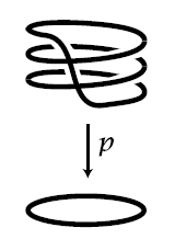
Regard the circle as the topological subspace of elements of unit absolute value in the complex plane. For , consider the continuous function
given by taking a complex number to its -th power. This may be thought of as the result of “winding the circle times around itself”. Precisely, this is a covering space (def. ) with leaves at each point.
graphics grabbed from Hatcher
Example
(covering of circle by real line)
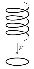
Consider the continuous function
from the real line to the circle, which,
-
with the circle regarded as the unit circle in the complex plane , is given by
-
with the circle regarded as the unit circle in , is given by
We may think of this as the result of “winding the line around the circle ad infinitum”. Precisely, this is a covering space (def. ) with the leaves at each point forming the set of integers.
Below in example we see that this is the universal covering space of the circle.
Here are some basic properties of covering spaces:
Proposition
(covering projections are open maps)
If is a covering space projection, then is an open map.
Proof
By definition of covering space there exists an open cover and homeomorphisms for all . Since the projections out of a product topological space are open maps (this prop.), it follows that is an open map when restricted to any of the . But a general open subset is the union of its restrictions to these subspaces:
Since images preserve unions (this prop.) it follows that
is a union of open sets, and hence itself open.
Lemma
(fiber-wise diagonal of covering space is open and closed)
Let be a covering space. Consider the fiber product
hence (by the discussion at Top - Universal constructions) the topological subspace of the product space , as shown on the right. By the universal property of the fiber product, there is the diagonal continuous function
Then the image of under this function is an open subset and a closed subset:
Proof
First to see that it is an open subset. It is sufficient to show that for any there exists an open neighbourhood of .
Now by definition of covering spaces, there exists an open neighbourhood of such that
It follows that is an open neighbourhood. Hence by the nature of the product topology, is an open neighbourhood of in and hence by the nature of the subspace topology the restriction
is an open neighbourhood of in .
Now to see that the diagonal is closed, hence that the complement is an open subset, it is sufficient to show that every point with but has an open neighbourhood in this complement.
As before, there is an open neighbourhood of over which the cover trivializes, and hence are open neighbourhoods of and , respectively. These are disjoint by the assumption that . As above, this means that the intersection
is an open subset of the complement of the diagonal in the fiber product.
Lifting properties
If is any continuous function (possibly a covering space or a topological vector bundle) then a section is a continuous function which sends each point in the base to a point in the fiber above it, hence which makes this diagram commute:
We may think of this as “lifting” each point in the base to point in the fibers “through” the projection map . More generally if is a subspace, we may consider such lifts only over
sometimes called a “local section”. But this suggests that for any continuous function, we consider “lifting its image through ”
For example if is the topological interval, then is a path in the base space , and a lift through of this is a path in the total space which “runs above” the given path. Such lifts of paths through covering projections is the topic of monodromy below.
Here it is of interest to consider the lifting problem subject to some constraint. For instance we will want to consider lifts of paths through a covering projection, subject to the condition that the starting point is lifted to a prescribed point .
Since such a point is equivalently a continuous function out of the point space, this is the same as asking for a continuous function that makes both triangles in the following diagram commute:
This is an example of a general situation which plays a central role in homotopy theory: We say that a square commuting diagram
is a lifting problem and that a diagonal morphism
such that both resulting triangles commute is a lift. If such a lift exists for for the given and for each taken from some class of morphisms, then one says that has the right lifting property against this class.
We now discuss some right lifting properties satisfied by covering spaces:
A first application of the lifting theorem is that it gives the concept of the universal covering space (def. , prop. below) which is central to the theory of covering spaces.
These lifting properties will be used in below for the computation of fundamental groups and higher homotopy groups of some topological spaces.
Lemma
(lifts out of connected space into covering spaces are unique relative to any point)
Let
-
be a covering space,
-
two lifts of , in that the following diagram commutes:
for .
If there exists such that then the two lifts already agree everywhere: .
Proof
By the universal property of the fiber product
the two lifts determine a single continuous function of the form
Write
for the diagonal on in the fiber product. By lemma this is an open subset and a closed subset of the fiber product space. Hence by continuity of also its pre-image
is both closed and open, hence also its complement is open in .
Moreover, the assumption that the functions and agree in at least one point means that the above pre-image is non-empty. Therefore the assumption that is connected implies that this pre-image coincides with all of . This is the statement to be proven.
Lemma
(path lifting property)
Let be any covering space. Given
-
a path in ,
-
be a lift of its starting point, hence such that
then there exists a unique path such that
-
it is a lift of the original path: ;
-
it starts at the given lifted point: .
In other words, every commuting diagram in Top of the form
has a unique lift:
Proof
First consider the case that the covering space is trivial, hence of the Cartesian product form
By the universal property of the product topological spaces in this case a lift is equivalently a pair of continuous functions
Now the lifting condition explicitly fixes . Moreover, a continuous function into a discrete topological space is locally constant, and since is a connected topological space this means that is in fact a constant function (this example), hence uniquely fixed to be .
This shows the statement for the case of trivial covering spaces.
Now consider any covering space . By definition of covering spaces, there exists for every point a open neighbourhood such that the restriction of to becomes a trivial covering space:
Consider such a choice
This is an open cover of . Accordingly, the pre-images
constitute an open cover of the topological interval .
Now the closed interval is a compact topological space, so that this cover has a finite open subcover. By the Euclidean metric topology, each element in this finite subcover is a disjoint union of open intervals. The collection of all these open intervals is an open refinement of the original cover, and by compactness it once more has a finite subcover, now such that each element of the subcover is guaranteed to be a single open interval.
This means that we find a finite number of points
with and such that for all there is such that the corresponding path segment
is contained in from above.
Now assume that has been found. Then by the triviality of the covering space over and the first argument above, there is a unique lift of to a continuous function with starting point . Since is the pushout (this example), it follows that and uniquely glue to a continuous function which lifts .
By induction over , this yields the required lift .
Conversely, given any lift, , then its restrictions are uniquely fixed by the above inductive argument. Therefore also the total lift is unique. Alternatively, uniqueness of the lifts is a special case of lemma .
Proposition
(homotopy lifting property of covering spaces)
Let
-
be a covering space;
Then every lifting problem of the form
has a unique lift
Proof
It is clear what the lift must be: For every point the situation restricts to that of path lifting
And so at each point the lift of must be the unique path that lifts this with starting point . We just need to see that this lift is a continuous function.
To that end we generalize he proof of the path lifting to connected open neighbourhoods of points in :
Let be an open cover over which the covering space trivializes. Then the pre-images is an open cover of the product space. By nature of the product space topology and the Euclidean topology on , each of the is a union of Cartesian products with an open subset of and an interval. Hence there is an open cover of the form
with the property that for each there exists with .
Now by the fact that is a compact topological space, for each there exists a finite set such that
still restricts to a cover of . Since is finite, the intersection
is still open, and so also
still restricts to a cover of .
This means that the same argument as for the path lifting in lemma provides a unique lift for each .
Moreover, for two points, these lifts clearly have to agree on .
Since is an open cover, means that there is a unique function that restricts to all these local lifts (this prop). This is the required lift.
Remark
(covering spaces are Hurewicz fibrations)
Continuous functions that satisfy the homotopy lifting property, hence that have the right lifting property against continuous functions of the form are called Hurewicz fibrations. Hence prop. says that covering projections are in particular Hurewicz fibrations.
Example
(homotopy lifting property for given lifts of paths relative starting point)
Let be a covering space. Then given a homotopy relative the starting point between two paths in ,
there is for every lift of these two paths to paths in with the same starting point a unique homotopy
between the lifted paths that lifts the given homotopy:
For commuting squares of the form
there is a unique diagonal lift in the lower diagram, as shown.
Moreover if the homotopy also fixes the endpoint, then so does the lifted homotopy .
Proof
There are horizontal homeomorphisms such that the following diagram commutes
Example
Let be a pointed covering space and let be a point-preserving continuous function such that the image of the fundamental group of is contained within the image of the fundamental group of in that of :
Then for a path in that happens to be a loop, every lift of its image path in to a path in is also a loop there.
Proof
By assumption, there is a loop in and a homotopy fixing the endpoints of the form
Then by the homotopy lifting property as in example , there is a homotopy in relative to the basepoint
and lifting the homotopy . Therefore is in fact a homotopy between loops, and so is indeed a loop.
Proposition
(lifting theorem)
Let
-
be a covering space;
-
a point, with denoting its image,
-
be a connected and locally path-connected topological space;
-
a point
-
a continuous function such that .
Then the following are equivalent:
-
There exists a unique lift in the diagram
-
The image of the fundamental group of under in that of is contained in the image of the fundamental group of under :
Moreover, if is path-connected, then the lift in the first item is unique.
Proof
The implication is immediate. We need to show that the second statement already implies the first.
So assume that . If a lift exists, then its uniqueness is given by lemma . Hence we need to exhibit a lift.
Since is connected and locally path-connected, it is also a path-connected topological space (this prop.). Hence for every point there exists a path connecting with and hence a path connecting with . By the path-lifting property (lemma ) this has a unique lift
Therefore
is a lift of .
We claim now that this pointwise construction is independent of the choice , and that as a function of it is indeed continuous. This will prove the claim.
First, by the path lifting lemma the lift is unique given , and hence depends at most on the choice of .
Hence let be another path in that connects with . We need to show that then .
First observe that if is related to by a homotopy, so that then also is related to by a homotopy, then this is the statement of the homotopy lifting property in the form of example .
Next write for the path concatenation of the path with the reverse path of the path . This is hence a loop in , and so is a loop in . The assumption that implies, via example , that the path which lifts this loop to is itself a loop in .
By uniqueness of path lifting, this means that the lift of
coincides at with that of at 1. But is homotopic (via reparameterization) to just . Hence it follows now with the first statement that the lift of indeed coincides with that of .
This shows that the above prescription for is well defined.
It only remains to show that the function obtained this way is continuous.
Let be a point and an open neighbourhood of its image in . It is sufficient to see that there is an open neighbourhood such that .
Let be an open neighbourhood over which trivializes. Then the restriction
is an open subset of the product space. Consider its further restriction
to the leaf
which is itself an open subset. Since is an open map (this prop.), the subset
is open, hence so is its pre-image
Since is assumed to be locally path-connected, there exists a path-connected open neighbourhood
By the uniqueness of path lifting, the image of that under is
This shows that the lifted function is continuous. Finally that this continuous lift is unique is the statement of lemma .
The lifting theorem implies that there are “universal” covering spaces:
Definition
A covering space is called a universal covering space if the total space is a simply connected topological space (def. )
It makes sense to speak of the universal covering space, because any two are isomorphic:
Proposition
(universal covering space is unique up to isomorphism)
For a locally path-connected topological space, then any two universal covering spaces over (def. ) are isomorphic.
Proof
Since both and are simply connected, the assumption of the lifting theorem for covering spaces is satisfied (prop. ). This says that there are horizontal continuous function making the following diagrams commute:
and that these are unique once we specify the image of a single point, which we may freely do (in the given fiber).
So if we pick any point and with and with and specify that and then uniqueness applied to the composites implies and .
Example
(universal covering space of the circle)
The real line, which is simply connected by example , equipped with the projection from example
is the (prop. ) universal covering space of the circle.
Monodromy
Since the lift of a path through a covering space projection is unique once the lift of the starting point is chosen (lemma ) every path in the base space determines a function between the fiber sets over its endpoints. By the homotopy lifting property of covering spaces as in example this function only depends on the equivalence class of the path under homotopy relative boundary. Therefore this fiber-assignment is in fact an action of the fundamental groupoid of the base space on sets, called a groupoid representation (def. below). In particular, associated with any homotopy-class of a loop, hence of an element in the fundamental group, there is associated a bijection of the fiber over the loop’s basepoint with itself, hence a permutation representation of the fundamental group. This is called the monodromy of the covering space. It is a measure for how the covering space fails to be globally trivial.
In fact the fundamental theorem of covering spaces (prop. ) below says that the monodromy representation characterizes the covering spaces completely and faithfully. This means that covering spaces may be dealt with completely with tools from group theory and representation theory, a fact that we make use of in the computation of examples below.
Definition
Let be a groupoid. Then:
A linear representation of is a groupoid homomorphism (functor)
to the groupoid core of the category Vect of vector spaces (example ). Hence this is
-
For each object of a vector space ;
-
for each morphism of a linear map
such that
-
(respect for composition) for all composable morphisms in the groupoid we have an equality
-
(respect for identities) for each object of the groupoid we have an equality
Similarly a permutation representation of is a groupoid homomorphism (functor)
to the groupoid core of Set. Hence this is
such that composition and identities are respected, as above.
For and two such representations, then a homomorphism of representations
is a natural transformation between these functors, hence is
-
for each object of the groupoid a (linear) function
-
such that for all morphisms we have
By def. the representations of in and homomorphisms between them constitute a groupoid called the representation groupoid
Example/Definition
(group representations are groupoid representations of delooping groupoids)
If is the delooping groupoid of a group (example ), then a groupoid representation of is a group representation of (def. ), and one writes
for the representation groupoid.
For each object the canonical inclusion of the delooping groupoid of the automorphism group (from def. )
induces by precomposition a homomorphism of representation groupoids:
We say that a groupoid representation is faithful or free if for all objects its restriction to a group representation of this way is transitive or free, respectively.
Here the representation of a group on some set
-
transitive if for all pairs of elements there is a such that ;
-
free if whenever holds for all then is the neutral elements.
Proposition
(groupoid representations are products of group representations)
Assuming the axiom of choice then the following holds:
Let be a groupoid. Then its groupoid of groupoid representations (def. ) is equivalent (def. ) to the product groupoid (example ) indexed by the set of connected components (def. ) of group representations (example ) of the automorphism group (def. ) for any object in the th connected component:
Proof
Let be the category that the representation is on (e.g. Set for permutation representations). Then by definition
Consider the injection functor of the skeleton from lemma
By lemma the pre-composition with this constitutes a functor
and by combining lemma with lemma this is an equivalence of groupoids. Finally, by example the groupoid on the right is the product groupoid as claimed.
Definition
(monodromy of a covering space)
Let be a topological space and a covering space (def. ). Write for the fundamental groupoid of (example ).
Define a groupoid homomorphism
to the groupoid core of the category Set of sets (example ), hence a permutation groupoid representation (example ), as follows:
-
to a point assign the fiber ;
-
to the homotopy class of a path connecting with in assign the function which takes to the endpoint of a path in which lifts through with starting point
This construction is well defined for a given representative due to the unique path-lifting property of covering spaces (lemma ) and it is independent of the choice of in the given homotopy class of paths due to the homotopy lifting property (example ). Similarly, these two lifting properties give that this construction respects composition in and hence is indeed a homomorphism of groupoids (a functor).
Proposition
(extracting monodromy is functorial)
Given a isomorphism between two covering spaces , hence a homeomorphism which respects fibers in that the diagram
commutes, then the component functions
are compatible with the monodromy (def. ) along any path between points and from def. in that the following diagrams of sets commute
This means that induces a homotopy (natural transformation) between the monodromy homomorphisms (functors)
of and , respectively, and hence that constructing monodromy is itself a homomorphism from the groupoid of covering spaces of to that of permutation representations of the fundamental groupoid of :
Proof
Let be an element, and a lift of to with . This means by definition of monodromy that
Since the function is compatible with the covering projections, the image is a lift of to , with . Therefore
In conclusion, for each element we have
This means that the square commutes, as claimed.
Example
(fundamental groupoid of covering space)
Let be a covering space.
Then the fundamental groupoid of the total space is the groupoid
whose
This is also called the Grothendieck construction of the monodromy functor , and denoted
Proof
By the uniqueness of the path-lifting, lemma and the very definition of the monodromy functor.
Example
(covering space is universal if monodromy is free and transitive)
Let be a path-connected topological space and let be a covering space. Then the total space is
-
path-connected precisely if the monodromy is a transitive action;
-
simply connected (def. ) hence universal covering space
(def. ) precisely if the monodromy is a transitive and free action.
Definition
(reconstruction of covering spaces from monodromy)
Let
Consider the disjoint union set of all the sets appearing in this representation
For
-
an open subset
-
which is path-connected
-
for which every element of the fundamental group becomes trivial under ,
-
-
for with
consider the subset
The collection of these defines a base for a topology (prop. below). Write for the corresponding topology. Then
is a topological space. It canonically comes with the function
Finally, for
a homomorphism of permutation representations, there is the evident induced function
Proposition
The construction in def. is well defined and yields a covering space of .
Moreover, the construction yields a homomorphism of covering spaces.
Proof
First to see that we indeed have a topology, we need to check (by this prop.) that every point is contained in some base element, and that every point in the intersection of two base elements has a base neighbourhood that is still contained in that intersection.
So let be a point. By the assumption that is semi-locally simply connected there exists an open neighbourhood such that every loop in on is contractible in . By the assumption that is a locally path-connected topological space, this contains an open neighbourhood which is path connected and, as every subset of , it still has the property that every loop in based on is contractible as a loop in . Now let be any point over , then it is contained in the base open .
The argument for the base open neighbourhoods contained in intersections is similar.
Then we need to see that is a continuous function. Since taking pre-images preserves unions (this prop.), and since by semi-local simply connectedness and local path connectedness every neighbourhood contains an open neighbourhood that labels a base open, it is sufficient to see that is a base open. But by the very assumption on , there is a unique morphism in from any point to any other point in , so that applied to these paths establishes a bijection of sets
thus exhibiting as a union of base opens.
Finally we need to see that this continuous function is a covering projection, hence that every point has a neighbourhood such that . But this is again the case for those all whose loops are contractible in , by the above identification via , and these exist around every point by semi-local simply-connectedness of .
This shows that is a covering space. It remains to see that is a homomorphism of covering spaces. Now by construction it is immediate that this is a function over , in that this diagram commutes:
So it only remains to see that is a continuous function. So consider a base open of . By naturality of
its pre-image under is
and hence a union of base opens.
Proposition
(fundamental theorem of covering spaces)
Let be a locally path-connected and semi-locally simply-connected topological space (def. ). Then the operations on
-
extracting the monodromy of a covering space over (def. , prop. )
-
reconstructing a covering space from monodromy (def. , prop. )
constitute an equivalence of groupoids (def.
between the groupoid (example , def. ) whose objects are covering spaces over , and whose morphisms are isomorphisms between these (def. ) and the groupoid of permutation groupoid representations (def. ) of the fundamental groupoid of (example ).
Proof
First we demonstrate a homotopy (natural isomorphism) of the form
To this end, given a permutation groupoid representation, we need to exhibit in turn a homotopy (natural isomorphism) of permutation representations.
First consider what the right hand side is like: By def. of and def. of we have for every an actual equality
To similarly understand the value of on morphisms , let be a representing path in . As in the proof of the path lifting lemma we find a finite number of paths such that
-
regarded as morphisms in they compose to :
-
each factors through an open subset over which trivializes.
Hence by functoriality of it is sufficient to understand its value on these paths . But on these we have again by direct unwinding of the definitions that
This means that if we take
to be the above identification, then this is a homotopy/natural isomorphism as required.
It remains to see that these morphism are themselves natural in , hence that for each morphism the diagram
commutes as a diagram in . Since these morphisms are themselves groupoid homotopies (natural isomorphisms) this is the case precisely if for all the corresponding component diagram commutes. But by the above this is
and hence this means that the top and bottom horizontal morphism are in fact equal. Direct unwinding of the definitions shows that this is indeed the case.
Now we demonstrate a homotopy (natural isomorphism) of the form
For a covering space, we need to exhibit a natural isomorphism of covering spaces of the form
Again by def. of and def. of the underlying set of is actually equal to that of , hence it is sufficient to check that this identity function on underlying sets is a homeomorphism of topological spaces.
By the assumption that is locally path-connected and semi-locally simply connected, it is sufficient to check for an open path-connected subset and a point with the property that lands is constant on the trivial element, that the open subsets of of the form form a basis for the topology of . But this is the case by definition of .
This proves the equivalence.
Example
(universal covering space reconstructed from free and transitive fundamental group representation)
Let be a topological space which is
Then a universal covering space of (def. ) exists.
Proof
By example the covering space is connected and simply connected precisely if its monodromy representation is free and transitive. By the fundamental theorem of covering spaces (prop. ) every permutation representation of the fundamental group arises as the monodromy of some covering space. Hence it remains to see that a free and transitive representation of exists: The action of any group on itself, by left multiplication, is free and transitive.
Examples
We now use the theorems established above to compute the fundamental groups of topological spaces in some basic examples. In particular we prove the archetypical example saying that the fundamental group of the circle is the integers (prop. below).
Fundamental groups
Proposition
(fundamental group of the circle is the integers)
The fundamental group of the circle is the additive group of integers:
and the isomorphism is given by assigning winding number.
Proof
By example , the universal covering space of is the real line
Since the circle is locally path-connected (this example) and semi-locally simply connected (this example) the fundamental theorem of covering spaces applies and gives that the automorphism group of over equals the automorphism group of its monodromy permutation representation:
Moreover, as a corollary of the fundamental theorem of covering spaces we have that the monodromy representation of a universal covering space is given by the action of the fundamental group on itself (this prop.).
But the automorphism group of any group regarded as an action on itself by left multiplication is canonically isomorphic to that group itself (by this example), hence we have
Therefore to conclude the proof it is now sufficient to show that
To that end, consider a homeomorphism of the form
Let be any point, and consider the restriction of to the fibers over the complement:
By the covering space property we have (via this example) a homeomorphism
Therefore, up to homeomorphism, the restricted function is of the form
By the universal property of the product topological space this means that is equivalently given by its two components
By the commutativity of the above diagram, the first component is fixed to be . Moreover, by the fact that is a discrete space it follows that the second component is a locally constant function (by this example). Therefore, since the product space with a discrete space is a disjoint union space (via this example)
and since the disjoint summands are connected topological spaces (this example), it follows that the second component is a constant function on each of these summands (by this example).
Finally, since every function out of a discrete topological space is continuous, it follows in conclusion that the restriction of to the fibers over is entirely encoded in an endofunction of the set of integers
by
Now let be another point, distinct from . The same analysis as above applies now to the restriction of to and yields a function
Since
is an open cover of , it follows that is uniquely fixed by its restrictions to these two subsets.
Now unwinding the definition of shows that the condition that the two restrictions coincide on the intersection implies that there is such that and .
This shows that .
Example
(isomorphism classes of coverings of the circle are conjugacy classes in the symmetric group)
The monodromy construction assigns to an isomorphism class of covering spaces over the circle with fibers consisting of elements conjugacy classes of elements the symmetric group :
To see this we may without restriction choose a basepoint so that a monodromy representation is equivalently a groupoid morphism of the form (prop. )
Since is the free abelian group on a single generator, such as morphism is uniquely determined by the image of . This is taken to some isomorphism of the set . If we choose any identification , then this defines an element in the symmetric group:
Now if
is an isomorphism of covering spaces, then by the fundamental theorem of covering spaces (prop. ) this corresponds bijectively to a homomorphism of representations
which in turn is by definition a homotopy (natural isomorphism) between the monodromy functors .
The combination of the naturality square of this natural isomorphism with the above identification yields the following diagram
The commutativity of the total rectangle says that the permutations and are related by conjugation with the element .
Example
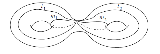
(three-sheeted covers of the circle)
Consider the three-sheeted covering spaces of the circle.
By example these are, up to isomorphism, given by the conjugacy classes of the elements of the symmetric group on three elements. These in turn are labeled by the cycle structure of the elements (this prop.).
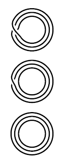
For the symmetric group on three elements there are three such classes
The corresponding covering spaces of the circle are shown in the graphics.
graphics grabbed from Hatcher
Higher homotopy groups
(…)
This concludes the introduction to basic homotopy theory.
For introduction to more general and abstract homotopy theory see at Introduction to Homotopy Theory.
An incarnation of homotopy theory in linear algebra is homological algebra. For introduction to that see at Introduction to Homological Algebra.
References
A textbook account:
- Tammo tom Dieck, sections 2 and 3 of Algebraic Topology, EMS 2006 (pdf, doi:10.4171/048)
Exposition:
-
Jesper Møller, The fundamental group and covering spaces (2011) [pdf, pdf]
-
Alberto Santini, Topological groupoids (2011) [pdf, pdf]
(about groupoids in topology, notably fundamental groupoids – not about topological groupoids)
Further reading:
Fun application of basic homotopy theory in condensed matter theory (anyon braiding):
- N. David Mermin, The topological theory of defects in ordered media, Rev. Mod. Phys. 51 (1979) 591 doi:10.1103/RevModPhys.51.591
Last revised on October 24, 2025 at 09:08:25. See the history of this page for a list of all contributions to it.