physics, mathematical physics, philosophy of physics
theory (physics), model (physics)
experiment, measurement, computable physics
Axiomatizations
Tools
Structural phenomena
Types of quantum field thories
synthetic differential geometry
Introductions
from point-set topology to differentiable manifolds
geometry of physics: coordinate systems, smooth spaces, manifolds, smooth homotopy types, supergeometry
Differentials
Tangency
The magic algebraic facts
Theorems
Axiomatics
Models
differential equations, variational calculus
Chern-Weil theory, ∞-Chern-Weil theory
Cartan geometry (super, higher)
In the context of electromagnetism, Maxwell’s equations are the equations of motion for the electromagnetic field strength electric current and magnetic current.
(This is the specialization of the Yang-Mills equations for the case that the structure group is abelian, see there).
is here the (vector of) strength of electric field and the strength of magnetic field; is the charge and the density of the electrical current; , , are constants (electrical permeability, speed of the light, and magnetic permeability; all of/in vacuum: ).
Gauss' law for electric fields
where is a closed surface which is a boundary of a 3d domain (physicists say “volume”) and the charge in the domain ; denotes the scalar (dot) product. Surface element is , i.e. it is the scalar surface measure times the unit vector of normal outwards.
No magnetic monopoles (Gauss’ law for magnetic fields)
where is any closed surface.
Faraday’s law of induction
The line element is the differential (or 1-d measure on the boundary) of the length times the unit vector in counter-circle direction (or parametrize the curve with being a vector in 3d space, express magnetic field in the same parameter and calculate the integral as a function of parameter: is a scalar (“dot”) product).
Ampère-Maxwell law (or generalized Ampère’s law; Maxwell added the second term involving derivative of the flux of electric field to the Ampère’s law which described the magnetic field due electric current).
where is a surface and its boundary; is the total current through (integral of the component of normal to the surface).
Here we put units with . By we denote the density of the charge.
In pregeometric form, Maxwell’s equations are differential equations for four fields (vector fields) called
electric field
magnetic flux density
magnetic field
displacement field (or similar)
and state:
(“there is no source for magnetic flux, hence no magnetic monopoles”)
Faraday’s law:
(“the source of electric flux is electric current”)
generalized Ampère’s law
In order to complete this pregeometric form to the actual equations of motion of the electromagnetic field, these four fields are to be subjected to a constraint called the constitutive equation which expresses as a function of .
In vacuum and in the absence of background gravity, this constitutive relation:
equates the displacement field with the electric field times a constant
called the “permitivity of the vacuum”,
equates the magnetic flux with the magnetic field times a constant
called the “permeability of the vacuum”.
But for electromagnetic fields inside dielectric media other constitutive relations appear. For small field strengths these are typically linear functions (e.g. de Lange & Raab 2006 (19))
but in general the constitutive relation can be a non-linear or even be a “multi-valued function” (namely when there are hysteresis effects in the dielectric medium).
Similarly (interestingly), in the presence of background gravity (such as for electromagnetic fields in and around a star) there is a linear such relation depending on the pseudo-Riemannian metric. This is most transparently expressed in terms of the Hodge star operator acting on the electromagnetic fields re-packaged as a Faraday tensor differential 2-form (see below).
This is adapted from electromagnetic field – Maxwell’s equations, for more see the references below.
In modern language, the insight of (Maxwell, 1865) is that locally, when physical spacetime is well approximated by a patch of its tangent space, i.e. by a patch of 4-dimensional Minkowski space , the electric field and magnetic field combine into a differential 2-form
in and the electric charge density and current density combine to a differential 3-form
in such that the following two equations of differential forms are satisfied
where is the de Rham differential operator and the Hodge star operator. If we decompose into its components as before as
then in terms of these components the Maxwell equations read as follows:
gives the magnetic Gauss law and Faraday’s law
gives Gauss's law and Ampère-Maxwell law
In the geometric algebra formalism of electromagnetism, one works in the 4-dimensional Clifford algebra representing spacetime, where the orthonormal basis vectors have signature with representing the time dimension and the other three basis vectors representing the spacial dimensions. The pseudoscalar of is represented by the product of all the basis vectors
The basis bivectors of come in two sets, the timelike bivectors , , , and the spacelike bivectors , , . The bivector subalgebra of is equivalent to the three-dimensional Clifford algebra corresponding to the relative space in the rest frame defined by , where the basis timelike bivectors correspond to the basis relative vectors and the basis spacelike bivectors correspond to the basis relative bivectors of the rest frame.
Let be a vector in . Then we define the coordinates of relative to the basis to be . is also denoted as since it represents the time coordinate. The spacetime vector derivative is defined as the operator
The relative vector derivative is defined as the operator
Assuming the use of natural units where and ignoring the polarization and magnatization fields for the time being, Maxwell’s equations are written as:
electric Gauss’s law:
Faraday’s law:
magnetic Gauss’s law:
Ampère-Maxwell law:
where and are the relative electric and magnetic relative fields, is the density of the charge, and is the relative current of the charge.
The Faraday bivector is the bivector . By multiplying the last two equations by the pseudoscalar, one gets
and by adding the four equations together, one gets the equation
which then becomes
Given a timelike bivector and a general bivector in , . Thus, the above equation could be simplified even further to
or
Now, the spacetime current is given by , which is a vector in spacetime. The spacetime vector derivative is related to the relative vector derivative by the following equation:
Thus, by left multiplying each side by , one gets
or
where is the spacetime vector derivative, is the Faraday bivector, and is the spacetime current.
For more see the references at electromagnetism.
Maxwell’s equations originate in:
James Clerk Maxwell, A Dynamical Theory of the Electromagnetic Field, Philosophical Transactions of the Royal Society of London 155 (1865) 459-512 [doi:10.1098/rstl.1865.0008, jstor:108892, Wikipedia entry]
James Clerk Maxwell, A Treatise on Electricity and Magnetism, Clarendon Press Series, Macmillan & Co. (1873), Cambridge University Press (2010) [ark:/13960/t9s17v886, doi:10.1017/CBO9780511709333, pdf, Wikipedia entry]
there written as a system of 20 equations. A historical account of how this came about:
The condensation of Maxwell’s 20 equations to the modern system of 4 equations (the two Gauss Laws, Faraday’s Law, and Ampère’s Law with Maxwell’s correction) is due, besides Heinrich Hertz, to the “Maxwellian’s” FitzGerald, Ledge and Oliver Heaviside?:
Some more history and reflection:
A. C. T. Wu, Chen Ning Yang: Evolution of the concept of vector potential in the description of the fundamental interactions, International Journal of Modern Physics A 21 16 (2006) 3235-3277 [doi:10.1142/S0217751X06033143]
Freeman J. Dyson, Why is Maxwell’s Theory so hard to understand?, Proceedings of The Second European Conference on Antennas and Propagation, EuCAP 2007 (doi: 10.1049/ic.2007.1146)
Chen Ning Yang, The conceptual origins of Maxwell’s equations and gauge theory, Phyics Today 67 11 (2014) [doi:10.1063/PT.3.2585, pdf]
See also:
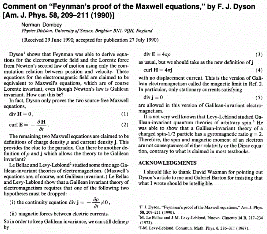
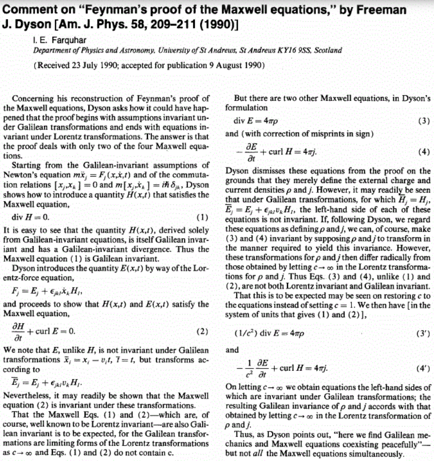
Freeman J. Dyson: Feynman’s proof of Maxwell’s equations, American Journal of Physics 58 (1990) 209-211 [pdf, pdf]
(recounting an observation by Richard Feynman)
comment by N. Dombey: Am. J. Phys. 59 1 (1991) 85 [journal, scan]
comment by I. E. Farquhar: Am. J. Phys. 59 1 (1991) 87 [journal, scan]
For Maxwell’s equations in the generality of dielectric media, see the references there, such as:
G. Russakoff, A Derivation of the Macroscopic Maxwell Equations, American Journal of Physics 38 (1970) 1188–1195 [doi:10.1119/1.1976000]
O. L. de Lange, R. E. Raab Surprises in the multipole description of macroscopic electrodynamics, American Journal of Physics 74 (2006) 301–312 [doi:10.1119/1.2151213]
On the Maxwell Green's function (propagator) and numerical solutions:
On the expression of classical electromagnetism, and especially of Maxwell's equations, in terms of differential forms, the de Rham differential and Hodge star operators:
Élie Cartan, §80 in: Sur les variétés à connexion affine, et la théorie de la relativité généralisée (première partie) (Suite), Annales scientifiques de l’É.N.S. 3e série, tome 41 (1924) 1-25 [numdam:ASENS_1924_3_41__1_]
(already in pregeometric form)
Charles Misner, Kip Thorne, John Wheeler, §3.4 and §4.3 in: Gravitation, W. H. Freeman, San Francisco (1973) [ISBN:9780716703440]
Theodore Frankel, Maxwell’s equations, The American Mathematical Monthly 81 4 (1974) [doi:10.1080/00029890.1974.11993557, jstor:2318995, doi:10.2307/2318995]
Walter Thirring, vol 2 §1.3 in: A Course in Mathematical Physics – 1 Classical Dynamical Systems and 2 Classical Field Theory, Springer (1978, 1992) [doi:10.1007/978-1-4684-0517-0]
Theodore Frankel, §§9-10 in: Gravitational Curvature, Freeman, San Francisco (1979) [ark:13960/t58d7nn19]
Dominic G. B. Edelen, §9.2 in: Applied exterior calculus, Wiley (1985) [GoogleBooks]
Theodore Frankel, §3.5 & §7.2b in: The Geometry of Physics - An Introduction, Cambridge University Press (1997, 2004, 2012) [doi:10.1017/CBO9781139061377]
Gregory L. Naber, §2.2 in: Topology, Geometry and Gauge fields – Interactions, Applied Mathematical Sciences 141 (2011) [doi:10.1007/978-1-4419-7895-0]
Masao Kitano, Reformulation of Electromagnetism with Differential Forms, Chapter 2 in: Trends in Electromagnetism – From fundamentals to applications, InTech (2012) 21-44 [ISBN:978-953-51-0267-0, pdf]
Sébastien Fumeron, Bertrand Berche, Fernando Moraes, Improving student understanding of electrodynamics: the case for differential forms, American Journal of Physics 88 (2020) 1083 [doi:10.1119/10.0001754, arXiv:2009.10356]
Formulation of Maxwell’s equations via “geometric algebra”:
Chris Doran, Anthony Lasenby: Geometric algebra for physicists, Cambridge University Press (2003) (pdf)
John W. Arthur, Understanding Geometric Algebra for Electromagnetic Theory, John Wiley & Sons Inc. (2011). (ISBN:978-0470941638, doi:10.1002/9781118078549)
Last revised on May 14, 2026 at 16:59:27. See the history of this page for a list of all contributions to it.