nLab geometry of physics -- coordinate systems

This entry is one chapter of the entry geometry of physics.

previous chapter: categories and toposes,

next chapter: smooth sets

As discussed in the chapter categories and toposes, every kind of geometry is modeled on a collection of archetypical basic spaces and geometric homomorphisms between them. In differential geometry the archetypical spaces are the abstract standard Cartesian coordinate systems, denoted $\mathbb{R}^n$ (in every dimension $n \in \mathbb{N}$). The geometric homomorphism between them are smooth functions $\mathbb{R}^{n_1} \to \mathbb{R}^{n_2}$, hence smooth (and possibly degenerate) coordinate transformations.

Here we introduce the basic concept, organizing them in the category CartSp of Cartesian spaces (Prop. below.) We highlight three classical theorems about smooth functions in Prop. below, which look innocent but play a decisive role in setting up synthetic differential supergeometry based on the concept of abstract smooth coordinate systems.

At this point these are not yet coordinate systems on some other space. But by applying the general machine of categories and toposes to these, a concept of generalized spaces modeled on these abstract coordinate systems is induced. These are the smooth sets discussed in the next chapter geometry of physics – smooth sets.

Abstract coordinate systems

In this Mod Layer we discuss the concrete particulars of coordinate systems: the continuum real line $\mathbb{R}$, the Cartesian spaces $\mathbb{R}^n$ formed from it and the smooth functions between these.

The continuum real line

The fundamental premise of differential geometry as a model of geometry in physics is the following.

Premise. The abstract worldline of any particle is modeled by the continuum real line $\mathbb{R}$.

This comes down to the following sequence of premises.

1. There is a linear ordering of the points on a worldline: in particular if we pick points at some intervals on the worldline we may label these in an order-preserving way by integers

   $\mathbb{Z}$.

2. These intervals may each be subdivided into $n$ smaller intervals, for each natural number $n$. Hence we may label points on the worldline in an order-preserving way by the rational numbers

   $\mathbb{Q}$.

3. This labeling is dense: every point on the worldline is the supremum of an inhabited bounded subset of such labels. This means that a worldline is the real line, the continuum of real numbers

   $\mathbb{R}$.

The adjective “real” in “real number” is a historical shadow of the old idea that real numbers are related to observed reality, hence to physics in this way. The experimental success of this assumption shows that it is valid at least to very good approximation.

Speculations are common that in a fully exact theory of quantum gravity, currently unavailable, this assumption needs to be refined. For instance in p-adic physics one explores the hypothesis that the relevant completion of the rational numbers as above is not the reals, but p-adic numbers $\mathbb{Q}_p$ for some prime number $p \in \mathbb{N}$. Or for example in the study of QFT on non-commutative spacetime one explore the idea that at small scales the smooth continuum is to be replaced by an object in noncommutative geometry. Combining these two ideas leads to the notion of non-commutative analytic space as a potential model for space in physics. And so forth.

For the time being all this remains speculation and differential geometry based on the continuum real line remains the context of all fundamental model building in physics related to observed phenomenology. Often it is argued that these speculations are necessitated by the very nature of quantum theory applied to gravity. But, at least so far, such statements are not actually supported by the standard theory of quantization: we discuss below in Geometric quantization how not just classical physics but also quantum theory, in the best modern version available, is entirely rooted in differential geometry based on the continuum real line.

This is the motivation for studying models of physics in geometry modeled on the continuum real line. On the other hand, in all of what follows our discussion is set up such as to be maximally independent of this specific choice (this is what topos theory accomplishes for us, discussed below Smooth spaces – Semantic Layer). If we do desire to consider another choice of archetypical spaces for the geometry of physics we can simply “change the site”, as discussed below and many of the constructions, propositions and theorems in the following will continue to hold. This is notably what we do below in Supergeometric coordinate systems when we generalize the present discussion to a flavor of differential geometry that also formalizes the notion of fermion particles: “differential supergeometry”.

Cartesian spaces and smooth functions

Definition

A function of sets $f : \mathbb{R} \to \mathbb{R}$ is called a smooth function if, coinductively:

1. the derivative $\frac{d f}{d x} : \mathbb{R} \to \mathbb{R}$ exists;

2. and is itself a smooth function.

We write $C^\infty(\mathbb{R}) \in Set$ for the set of all smooth functions on $\mathbb{R}$.

Remark

The superscript “${}^\infty$” in “$C^\infty(\mathbb{R})$” refers to the order of the derivatives that exist for smooth functions. More generally for $k \in \mathbb{N}$ one writes $C^k(\mathbb{R})$ for the set of $k$-fold differentiable functions on $\mathbb{R}$. These will however not play much of a role for our discussion here.

Definition

For $n \in \mathbb{N}$, the Cartesian space $\mathbb{R}^n$ is the set

$$\mathbb{R}^n = \{ (x^1 , \cdots, x^{n}) | x^i \in \mathbb{R} \}$$

of $n$-tuples of real numbers. For $1 \leq k \leq n$ write

$$i^k : \mathbb{R} \to \mathbb{R}^n$$

for the function such that $i^k(x) = (0, \cdots, 0,x,0,\cdots,0)$ is the tuple whose $k$th entry is $x$ and all whose other entries are $0 \in \mathbb{R}$; and write

$$\mathbb{p}^k : \mathbb{R}^n \to \mathbb{R}$$

for the function such that $p^k(x^1, \cdots, x^n) = x^k$.

A homomorphism of Cartesian spaces is a smooth function

$$f : \mathbb{R}^{n_1} \to \mathbb{R}^{n_2} \,,$$

hence a function $f : \mathbb{R}^{n_1} \to \mathbb{R}^{n_2}$ such that all partial derivatives exist and are continuous (…).

Example

Regarding $\mathbb{R}^n$ as an $\mathbb{R}$-vector space, every linear function $\mathbb{R}^{n_1} \to \mathbb{R}^{n_2}$ is in particular a smooth function.

Remark

But a homomorphism of Cartesian spaces in def. is not required to be a linear map. We do not regard the Cartesian spaces here as vector spaces.

Definition

A smooth function $f : \mathbb{R}^{n_1} \to \mathbb{R}^{n_2}$ is called a diffeomorphism if there exists another smooth function $\mathbb{R}^{n_2} \to \mathbb{R}^{n_1}$ such that the underlying functions of sets are inverse to each other

$$f \circ g = id$$

and

$$g \circ f = id \,.$$

Proposition

There exists a diffeomorphism $\mathbb{R}^{n_1} \to \mathbb{R}^{n_2}$ precisely if $n_1 = n_2$.

Definition

We will also say equivalently that

1. a Cartesian space $\mathbb{R}^n$ is an abstract coordinate system;

2. a smooth function $\mathbb{R}^{n_1} \to \mathbb{R}^{n_2}$ is an abstract coordinate transformation;

3. the function $p^k : \mathbb{R}^{n} \to \mathbb{R}$ is the $k$th coordinate of the coordinate system $\mathbb{R}^n$. We will also write this function as $x^k : \mathbb{R}^{n} \to \mathbb{R}$.

4. for $f : \mathbb{R}^{n_1} \to \mathbb{R}^{n_2}$ a smooth function, and $1 \leq k \leq n_2$ we write

   1. $f^k \coloneqq p^k\circ f$

   2. $(f^1, \cdots, f^n) \coloneqq f$.

Remark

It follows with this notation that

$$id_{\mathbb{R}^n} = (x^1, \cdots, x^n) : \mathbb{R}^n \to \mathbb{R}^n \,.$$

Hence an abstract coordinate transformation

$$f : \mathbb{R}^{n_1} \to \mathbb{R}^{n_2}$$

may equivalently be written as the tuple

$$\left( f^1 \left( x^1, \cdots, x^{n_1} \right) , \cdots, f^{n_2}\left( x^1, \cdots, x^{n_1} \right) \right) \,.$$

The magic properties of smooth functions

Below we encounter generalizations of ordinary differential geometry that include explicit “infinitesimals” in the guise of infinitesimally thickened points, as well as “super-graded infinitesimals”, in the guise of superpoints (necessary for the description of fermion fields such as the Dirac field). As we discuss below, these structures are naturally incorporated into differential geometry in just the same way as Grothendieck introduced them into algebraic geometry (in the guise of “formal schemes”), namely in terms of formally dual rings of functions with nilpotent ideals. That this also works well for differential geometry rests on the following three basic but important properties, which say that smooth functions behave “more algebraically” than their definition might superficially suggest:

Proposition

(the three magic algebraic properties of differential geometry)

1. embedding of Cartesian spaces into formal duals of R-algebras

   For $X$ and $Y$ two Cartesian spaces, the smooth functions $f \colon X \longrightarrow Y$ between them (def. ) are in natural bijection with their induced algebra homomorphisms $C^\infty(X) \overset{f^\ast}{\longrightarrow} C^\infty(Y)$ (example ), so that one may equivalently handle Cartesian spaces entirely via their $\mathbb{R}$-algebras of smooth functions.

   Stated more abstractly, this means equivalently that the functor $C^\infty(-)$ that sends a smooth manifold $X$ to its $\mathbb{R}$-algebra $C^\infty(X)$ of smooth functions (example ) is a fully faithful functor:

   $$C^\infty(-) \;\colon\; SmthMfd \overset{\phantom{AAAA}}{\hookrightarrow} \mathbb{R} Alg^{op} \,.$$

   (Kolar-Slovak-Michor 93, lemma 35.8, corollaries 35.9, 35.10)

2. embedding of smooth vector bundles into formal duals of R-algebra modules

   For $E_1 \overset{vb_1}{\to} X$ and $E_2 \overset{vb_2}{\to} X$ two vector bundle (def. ) there is then a natural bijection between vector bundle homomorphisms $f \colon E_1 \to E_2$ and the homomorphisms of modules $f_\ast \;\colon\; \Gamma_X(E_1) \to \Gamma_X(E_2)$ that these induces between the spaces of sections (example ).

   More abstractly this means that the functor $\Gamma_X(-)$ is a fully faithful functor

   $$\Gamma_X(-) \;\colon\; VectBund_X \overset{\phantom{AAAA}}{\hookrightarrow} C^\infty(X) Mod$$

   (Nestruev 03, theorem 11.29heorem#Nestruev03))

   Moreover, the modules over the $\mathbb{R}$-algebra $C^\infty(X)$ of smooth functions on $X$ which arise this way as sections of smooth vector bundles over a Cartesian space $X$ are precisely the finitely generated free modules over $C^\infty(X)$.

   (Nestruev 03, theorem 11.32heorem#Nestruev03))

3. vector fields are derivations of smooth functions.

   For $X$ a Cartesian space (example ), then any derivation $D \colon C^\infty(X) \to C^\infty(X)$ on the $\mathbb{R}$-algebra $C^\infty(X)$ of smooth functions (example ) is given by differentiation with respect to a uniquely defined smooth tangent vector field: The function that regards tangent vector fields with derivations from example

   $$\array{ \Gamma_X(T X) &\overset{\phantom{A}\simeq\phantom{A}}{\longrightarrow}& Der(C^\infty(X)) \\ v &\mapsto& D_v }$$

   is in fact an isomorphism.

   (This follows directly from the Hadamard lemma.)

Actually all three statements in prop. hold not just for Cartesian spaces, but generally for smooth manifolds (def./prop. below; if only we generalize in the second statement from free modules to projective modules. However for our development here it is useful to first focus on just Cartesian spaces and then bootstrap the theory of smooth manifolds and much more from that, which we do below.

The category of abstract coordinate systems

Here we make explicit the category formed by abstract coordinate systems (Prop. below) and mention some of its basic properties. This will serve the discussion of smooth sets as the sheaves on the category of abstract coordinate systems, in the next chapter geometry of physics – smooth sets.

$\,$

Propositions

(the category CartSp of abstract coordinate systems/Cartesian spaces)

Abstract coordinate systems according to prop. form a category (this def.) – to be denoted CartSp – whose

• objects are the abstract coordinate systems $\mathbb{R}^{n}$ (the class of objects is the set $\mathbb{N}$ of natural numbers $n$);

• morphisms$f : \mathbb{R}^{n_1} \to \mathbb{R}^{n_2}$ are the abstract coordinate transformations = smooth functions.

Composition of morphisms is given by composition of functions.

Under this identification

1. The identity morphisms are precisely the identity functions.

2. The isomorphisms are precisely the diffeomorphisms.

Definition

(opposite category of CartSp)

Write CartSp${}^{op}$ for the opposite category (this def.) of CartSp (Prop. ).

This is the category with the same objects as $CartSp$, but where a morphism $\mathbb{R}^{n_1} \to \mathbb{R}^{n_2}$ in $CartSp^{op}$ is given by a morphism $\mathbb{R}^{n_1} \leftarrow \mathbb{R}^{n_2}$ in $CartSp$.

We will be discussing below the idea of exploring smooth spaces by laying out abstract coordinate systems in them in all possible ways. The reader should begin to think of the sets that appear in the following definition as the set of ways of laying out a given abstract coordinate systems in a given space. This is discussed in more detail below in Smooth spaces.

Definition

A functor $X : CartSp^{op} \to Set$ (a “presheaf”) is

1. for each abstract coordinate system $U$ a set $X(U)$

2. for each coordinate transformation $f : \mathbb{R}^{n_1} \to \mathbb{R}^{n_2}$ a function $X(f) : X(\mathbb{R}^{n_1}) \to X(\mathbb{R}^{n_2})$

such that

1. identity is respected $X(id_{\mathbb{R}^n}) = id_{X(\mathbb{R}^n)}$;

2. composition is respected $X(f_2)\circ X(f_1) = X(f_2 \circ f_1)$

Example

Let $\mathcal{C}$ be a category.

1. The following are equivalent:

   1. $\mathcal{C}$ has a terminal object;

   2. the unique functor $\mathcal{C} \to \ast$ to the terminal category has a right adjoint

      $$\ast \underoverset {\underset{}{\longrightarrow}} {\overset{}{\longleftarrow}} {\bot} \mathcal{C}$$

   Under this equivalence, the terminal object is identified with the image under the right adjoint of the unique object of the terminal category.

2. Dually, the following are equivalent:

   1. $\mathcal{C}$ has an initial object;

   2. the unique functor $\mathcal{C} \to \ast$ to the terminal category has a left adjoint

      $$\mathcal{C} \underoverset {\underset{}{\longrightarrow}} {\overset{}{\longleftarrow}} {\bot} \ast$$

   Under this equivalence, the initial object is identified with the image under the left adjoint of the unique object of the terminal category.

Proof

Since the unique hom-set in the terminal category is the singleton, the hom-isomorphism characterizing the adjoint functors is directly the universal property of an initial object in $\mathcal{C}$

$$Hom_{\mathcal{C}}( L(\ast) , X ) \;\simeq\; Hom_{\ast}( \ast, R(X) ) = \ast$$

or of a terminal object

$$Hom_{\mathcal{C}}( X , R(\ast) ) \;\simeq\; Hom_{\ast}( L(X), \ast ) = \ast \,,$$

respectively.

The algebraic theory of smooth algebras

Propositions

• The category CartSp has all finite

products.

• Every object is a finite product of the object $\mathbb{R}$ (the real line itself).

• The terminal object is $\mathbb{R}^0$, the point.

Hence CartSp is (the syntactic category) of an algebraic theory (a Lawvere theory).

This is called the theory of smooth algebras.

Definition

A product-preserving functor

$$A : CartSp \to Set$$

is a smooth algebra. A homomorphism of smooth algebras is a natural transformation between the corresponding functors.

The basic example is:

Example

For $n \in \mathbb{N}$, the smooth algebra $C^\infty(\mathbb{R}^n)$ is the functor $CartSp \to Set$ which is functor corepresented by $\mathbb{R}^n \in$ CartSp. This means that to $\mathbb{R}^k \in CartSp$ it assigns the set

$$Hom_{CartSp}(\mathbb{R}^n , \mathbb{R}^k) = C^\infty(\mathbb{R}^n, \mathbb{R}^k)$$

of smooth functions from $\mathbb{R}^n$ to $\mathbb{R}^k$, and to a smooth function $f \colon \mathbb{R}^{k_1} \to \mathbb{R}^{k_2}$ it assigns the function

$$f\circ (-) \colon C^\infty(\mathbb{R}^n, \mathbb{R}^{k_1}) \to C^\infty(\mathbb{R}^n, \mathbb{R}^{k_2})$$

given by postcomposition with $f$.

Remark

Example shows how we are to think of a functor $A \colon CartSp \to Set$ as encoding an algebra: such a functor assigns to $\mathbb{R}^n$ a set to be interpreted as a set of “smooth functions on something with values in $\mathbb{R}^n$”, only that the “something” here is not pre-defined, but is instead indirectly characterized by this assignment.

Due to this we will often denote smooth algebras as “$C^\infty(X)$”, even if “$X$” is not a pre-defined object, and write their value on $\mathbb{R}^n$ as $C^\infty(X,\mathbb{R}^n)$.

This is illustrated by the next example.

Example

The smooth algebra of dual numbers $C^\infty(\mathbf{D})$ is the smooth algebra which assigns to $\mathbb{R}^n$ the Cartesian product

$$C^\infty(D,\mathbb{R}^n) \coloneqq \mathbb{R}^n \times \mathbb{R}^n$$

of two copies of $\mathbb{R}^n$, which we will write as

$$\left\{ (\epsilon \mapsto (\vec x + \epsilon \vec v)) | \vec x , \vec v \in \mathbb{R}^n \right\} \,.$$

Moreover, a smooth function $f \colon \mathbb{R}^{n_1} \to \mathbb{R}^{n_2}$ is sent to the function

$$C^\infty(D, f) \colon C^\infty(D, \mathbb{R}^{n_1}) \to C^\infty(D, \mathbb{R}^{n_2})$$

given by

$$\begin{aligned} \left(\epsilon \mapsto \left(\vec x + \epsilon \vec v\right)\right) \\ \left( \epsilon \mapsto f(\vec x) + (\mathbf{d}f)(\vec v) \right) &\mapsto \left( \epsilon \mapsto \left( f\left(\vec x\right) + \sum_{j = 1}^{n_2} \left(\sum_{i = 1}^{n_1}\frac{\partial f^j}{\partial x^i} v^i\right) \vec e_j \right) \right) \end{aligned} \,.$$

Remark

As the notation suggests, we may think of $C^\infty(D)$ as the functions on a first order infinitesimal neighbourhood of the origin in $\mathbb{R}^n$.

The coverage of differentially good open covers

We discuss a standard structure of a site on the category CartSp. Following Johnstone – Sketches of an Elephant, it will be useful and convenient to regard a site as a (small) category equipped with a coverage. This generates a genuine Grothendieck topology, but need not itself already be one.

Definition

For $n \in \mathbb{N}$ the standard open n-ball is the subset

$$D^n = \{ (x_i)_{i =1}^n \in \mathbb{R}^n | \sum_{i = 1}^n (x_i)^2 \lt 1 \} \hookrightarrow \mathbb{R}^n \,.$$

Proposition

There is a diffeomorphism

$$\mathbb{R}^n \stackrel{\simeq}{\to} D^n \,.$$

Definition

A differentially good open cover of a Cartesian space $\mathbb{R}^n$ is a set $\{U_i \hookrightarrow \mathbb{R}^n\}$ of open subset inclusions of Cartesian spaces such that these cover $\mathbb{R}^n$ and such for each non-empty finite intersection there exists a diffeomorphism

$$\mathbb{R}^n \stackrel{\simeq}{\to} U_{i_1} \cap \cdots \cap U_{i_k}$$

that identifies the $k$-fold intersection with a Cartesian space itself.

Remark

Differentiably good covers are useful for computations. Their full impact is however on the homotopy theory of simplicial presheaves over CartSp. This we discuss in the chapter on smooth homotopy types, around this prop.omotopy types#DifferentiablyGoodCoverGivesSPlitHyperCoverOverCartSp).

Proposition

Every open cover refines to a differentially good open cover, def. .

A proof is at good open cover.

Remark

Despite its appearance, this is not quite a classical statement. The classical statement is only that every open cover is refined by a topologically good open cover. See the comments here in the references-section at open ball for the situation concerning this statement in the literature.

Remark

The good open covers do not yet form a Grothendieck topology on CartSp. One of the axioms of a Grothendieck topology is that for every covering family also its pullback along any morphism in the category is a covering family. But while the pullback of every open cover is again an open cover, and hence open covers form a Grothendieck topology on CartSp, not every pullback of a good open cover is again good.

Example

Let $\{\mathbb{R}^2\stackrel{\phi_{i}}{\hookrightarrow}\mathbb{R}^2\}_{i \in \{1,2\}}$ be the open cover of the plane by an open left half space

$$\mathbb{R}^2 \simeq \{ (x_1,x_2) \in \mathbb{R}^2 | x_1 \lt 1 \} \stackrel{\phi_1}{\hookrightarrow} \mathbb{R}^2$$

and a right open half space

$$\mathbb{R}^2 \simeq \{ (x_1,x_2) \in \mathbb{R}^2 | x_1 \gt -1 \} \stackrel{\phi_2}{\hookrightarrow} \mathbb{R}^2 \,.$$

The intersection of the two is the open strip

$$\mathbb{R}^2 \simeq \{ (x_1, x_2) \in \mathbb{R}^2 | -1 \lt x_1 \lt 1 \} \hookrightarrow \mathbb{R}^2 \,.$$

So this is a good open cover of $\mathbb{R}^2$.

But consider then the smooth function

$$2(\cos(2 \pi (-)), \sin(2 \pi (-))) \colon \mathbb{R}^1 \to \mathbb{R}^2$$

which sends the line to a curve in the plane that periodically goes around the circle of radius 2 in the plane.

Then the pullback of the above good open cover on $\mathbb{R}^2$ to $\mathbb{R}^1$ along this function is an open cover of $\mathbb{R}$ by two open subsets, each being a disjoint union of countably many open intervals in $\mathbb{R}$. Each of these open intervals is an open 1-ball hence diffeomorphic to $\mathbb{R}^1$, but their disjoint union is not contractible (it does not contract to the point, but to many points!).

So the pullback of the good open cover that we started with is an open cover which is not good anymore. But it has an evident refinement by a good open cover.

This is a special case of what the following statement says in generality.

Proposition

The differentially good open covers, def. , constitute a coverage on CartSp.

Hence CartSp equipped with that coverage is a site.

Proof

By definition of coverage we need to check that for $\{U_i \hookrightarrow \mathbb{R}^n\}_{i \in I}$ any good open cover and $f \colon \mathbb{R}^k \to \mathbb{R}^n$ any smooth function, we can find a good open cover $\{K_j \to \mathbb{R}^k\}_{j \in J}$ and a function $J \to I$ such that for each $j \in J$ there is a smooth function $\phi \colon K_j \to U_{\rho(j)}$ that makes this diagram commute:

$$\array{ K_j &\stackrel{\phi}{\to}& U_{i(j)} \\ \downarrow && \downarrow \\ \mathbb{R}^k &\stackrel{f}{\to}& \mathbb{R}^n } \,.$$

To obtain this, let $\{f^* U_i \to \mathbb{R}^k\}$ be the pullback of the original covering family, in that

$$f^* U_i \coloneqq \{ x \in \mathbb{R}^k | f(x) \in U_i \} \hookrightarrow \mathbb{R}^k \,.$$

This is evidently an open cover, albeit not necessarily a good open cover. But by prop. there does exist a good open cover $\{\tilde K_{\tilde j} \hookrightarrow \mathbb{R}^k\}_{\tilde j \in \tilde J}$ refining it, which in turn means that for all $\tilde j$ there is

$$\array{ \tilde K_{\tilde j} &\to& K_{j(\tilde j)} \\ \downarrow && \downarrow \\ \mathbb{R}^k &\stackrel{=}{\to}& \mathbb{R}^k } \,.$$

Therefore then the pasting composite of these commuting squares

$$\array{ \tilde K_{\tilde j} &\to& K_{j(\tilde j)} &\to& U_{i(j(\tilde j))} \\ \downarrow && \downarrow && \downarrow \\ \mathbb{R}^k &\stackrel{=}{\to}& \mathbb{R}^k &\stackrel{f}{\to}& \mathbb{R}^n }$$

solves the condition required in the definition of coverage.

By example this good open cover coverage is not a Grothendieck topology. But as any coverage, it uniquely completes to one which has the same sheaves.

Proposition

The Grothendieck topology induced on CartSp by the differentially good open cover coverage of def. has as covering families the ordinary open covers.

Remark

This means that for every sheaf-theoretic construction to follow we can just as well consider the Grothendieck topology of open covers on $CartSp$. The sheaves of the open cover topology are the same as those of the good open cover coverage. But the latter is (more) useful for several computational purposes in the following. It is the good open cover coverage that makes manifest, below, that sheaves on $CartSp$ form a locally connected topos and in consequence then a cohesive topos. This kind of argument becomes all the more pronounced as we pass further below to (∞,1)-sheaves on CartSp. This will be discussed in Smooth n-groupoids – Semantic Layer – Local Infinity-Connectedness below.

The slice category

(…)

• slice category$CartSp_{\mathbb{R}^n}$

• subterminal object, open cover

(…)

$\,$

Syntactic Layer

In this Syn Layer we discuss the abstract generals of abstract coordinate systems, def. : the internal language of a category with products, which is type theory with product types.

This is rough, needs further development.

Judgments about types and terms

We now introduce a different notation for objects and morphisms in a category (such as the category CartSp of def. ). This notation is designed to, eventually, make more transparent what exactly it is that happens when we reason deductively about objects and morphisms of a category.

But before we begin to make any actual deductions about objects and morphisms in a category below, in this section here we express the given objects and morphisms at hand in the first place. Such basic statements of the form “There is an object called $A$” are to be called judgments, in order not to confuse these with genuine propositions that we eventually formalize within this metalanguage.

To express that there is an object

$$X \in \mathcal{C}$$

in a category $\mathcal{C}$, we write now equivalently the string of symbols (called a sequent)

$$\vdash \; X \colon Type \,.$$

We say that these symbols express the judgment that $X$ is a type. We also say that $\vdash \; X \colon Type$ is the syntax of which $X \in \mathcal{C}$ is the categorical semantics.

For instance the terminal object $* \in \mathcal{C}$ we call the categorical semantics of the unit type and write syntactically as

$$\vdash \; Unit \colon Type \,.$$

If we want to express that we do assume that a terminal object indeed exists, hence that we want to be able to deduce the existence of a terminal object from no hypothesis, then we write this judgment below a horizontal line

$$\frac{}{\vdash \; Unit \colon Type} \,.$$

We will see more interesting such horizontal-line statements below.

Next, to express an element of the object $X$ in $\mathcal{C}$, hence a morphism

$$* \stackrel{x}{\to} X$$

in $\mathcal{C}$ we write equivalently the sequent

$$\vdash \; x \colon X$$

and call this the judgment that $x$ is a term of type $X$.

Notice that every object $X \in \mathcal{C}$ becomes the terminal object in the slice category $\mathcal{C}_{/X}$. Let $A \to X$ be any morphism in $\mathcal{C}$, regarded as an object in the slice category

$$A \in \mathcal{C}_{/X} \,.$$

We declare that the syntax of which this is the categorical semantics is given by the sequent

$$x \colon X \;\vdash \; A(x) \colon Type \,.$$

We say that this expresses the judgement that $A$ is an $X$-dependent type; or a type in the context of a free variable $x$ of type $X$.

Notice that an element of $A \in \mathcal{C}_{/X}$ is a generalized element of $A$ in $\mathcal{C}$, namely a morphism $X \to A$ which fits into a commuting diagram

$$\array{ X &&\stackrel{a}{\to}&& A \\ & {}_{\mathllap{id_X}}\searrow && \swarrow_{} \\ && X }$$

in $\mathcal{C}$.

We declare that the syntax of which such

$$a \in A \;\;\;\; (in \mathcal{C}_{/X})$$

is this the categorical semantics is the sequent

$$x\colon X \;\vdash\; a(x) : A(x) \,.$$

We say that this expresses the judgment that $a(x)$ is a term depending on the free variable $x$ of type $X$.

This completes the list of judgment syntax to be considered. Notice that if the category $\mathcal{C}$ has products then, even though it does not explicitly appear above, this is sufficient to express any morphism $X \stackrel{f}{\to} Y$ in $\mathcal{C}$ as the semantics of a term: we regard this morphism naturally as being the corresponding morphism in the slice category $\mathcal{C}_{/X}$ which as a commuting diagram in $\mathcal{C}$ itself is

$$\array{ X && \stackrel{(f,id_X)}{\to} && Y\times X \\ & {}_{\mathllap{id_X}}\searrow && \swarrow_{\mathrlap{p_2}} \\ && X } \,.$$

This is the categorical semantics for which the syntax is simply

$$x \colon X \;\vdash\; y(x) \colon Y \,,$$

being the judgment which expresses that $y(x)$ is a term in context of an $X$-dependent type $Y$ in the special degenerate case that $Y$ does not actually vary with $x \colon X$.

Natural deduction rules for product types

With the above symbolic notation for making judgments about the presence of objects and morphisms in a category $\mathcal{C}$, we now consider a system of rule of deduction that tells us how we may process these symbols (how to do computations) such that the new symbols we obtain in turn express new objects and new morphisms in $\mathcal{C}$ that we can build out of the given ones by universal constructions in the sense of category theory.

This way of deducing new expressions from given ones is very basic as well as very natural and hence goes by the technical term natural deduction. For every kind of type (every universal construction in category theory) there is, in natural deduction, one set of rules for how to deductively reason about it. This set of rules, in turn, always consists of four kinds of rules, called the

1. type formation rule

2. term introduction rule

3. term elimination rule

4. computation rule.

These are going to be the syntax in type theory of which universal constructions in category theory is the categorical semantics.

In our running example where $\mathcal{C} =$ CartSp, the only universal construction available is that of forming products. We therefore introduce now the natural deduction rules by way of example of the special case of product types.

1. type formation rule Let

$$A , B \in \mathcal{C}$$

be two objects in a category with products. Then there exists the product object

$$A \times B \in \mathcal{C} \,.$$

We now declare that the syntax of which this state of affairs is the categorical semantics is the collection of symbols of the form

$$\frac{A \colon Type \;\;\;\;\; B \colon Type}{ A \times B \colon Type} \,.$$

Here on top of the horizontal line we have the two judgments which express that, syntactically, $A$ is a type and $B$ is a type, and semantically that $A \in \mathcal{C}$ and $B \in \mathcal{C}$. Below the horizontal line is, in turn, the judgment which expresses that there is, syntactically, a product type, which semantically is the product $A \times B \in \mathcal{C}$. The horizontal line itself is to indicate that if we are given the (symbols of) the collection of judgments on top, then we are entitled to also obtain the judgment on the bottom.

Remark (Computation) All this may seem, on first sight, like being a lot of fuss about something of grandiose banality. To see what is gradually being accomplished here despite of this appearance, as we proceed in this discussion, the reader can and should think of this as the first steps in the definition of a programming language: the notion of judgment is a syntactic rule for strings of symbols that a computer is to read in, and a natural deduction-step as the type formation rule above is an operation that this computer validates as being an allowed step of transforming a memory state with a given collection of such strings into a new memory state to which the string below the horizontal line is added. As we add the remaining rules below, what looks like a grandiose banality so far will remain grandiose, but no longer be a banality. The reader feeling in need of more motivational remarks along these lines might want to take a break here and have a look at the entry computational trinitarianism first, that provides more pointers to the grandiose picture which we are approaching here.

Next, the second natural deduction rule for product types is the

2. term elimination rule. The fact that $A \times B \in \mathcal{C}$ is equipped with two projection morphisms

$$\array{ A \stackrel{p_1}{\leftarrow} A \times B \stackrel{p_2}{\to} B }$$

means that from every element $t$ of $A \times B$ we may deduce the existence of elements $p_1(t)$ and $p_2(t)$ of $A$ and $B$, respectively. We declare now that this is the categorical semantics of which the natural deduction syntax is:

$$\frac{\vdash \; t \colon A \times B}{\vdash \; p_1(t) \colon A} \;\;\;\;\;\;\;\;\; \frac{\vdash \; t \colon A \times B}{\vdash \; p_2(t) \colon B} \,.$$

As before, this is to say that if syntactically we are given strings of symbols expressing judgments as on the top of these horizontal lines, then we may “naturally deduce” also the judgment of the string of symbols on the bottom of this line.

3. term introduction rule. The first part of the universal property of the product in category theory is that for $Q \in \mathcal{C}$ any other object equipped with morphisms

$$\array{ && Q \\ & {}^{\mathllap{a}}\swarrow && \searrow^{\mathrlap{b}} \\ A && && B }$$

in $\mathcal{C}$, we obtain a canonical morphism

$$Q \to A \times B$$

in $\mathcal{C}$. This is now declared to be the categorical semantics of which the natural deduction syntax is

$$\frac{ \vdash\; a \colon A \;\;\;\;\;\; \vdash\; b \colon B }{ \vdash (a,b) \colon A \times B } \,.$$

With the elements that are the semantics of the terms appearing here made explicit, this is the syntax for a diagram

$$\array{ && Q \\ & {}^{\mathllap{a}}\swarrow &\downarrow^{\mathrlap{(a,b)}}& \searrow^{\mathrlap{b}} \\ A && A \times B && B } \,.$$

4. computation rule. The next part of the universal property of the product in category theory is that the resulting diagram

$$\array{ && Q \\ & {}^{\mathllap{a}}\swarrow &\downarrow& \searrow^{\mathrlap{b}} \\ A &\stackrel{p_1}{\leftarrow}& A \times B & \stackrel{p_2}{\to} & B }$$

is in fact a commuting diagram. Syntactically this is, clearly, the rule that the following identifications of strings of symbols are to be enforced

$$p_1(a,b) = a \;\;\;\;\;\; p_2(a,b) = b \,.$$

This concluces the description of the natural deduction about objects, morphisms and products in a category using its type theory syntax. We summarize the dictionary between category theory and type theory discussed so far below.

In the next section we promote our running example category $\mathcal{C}$, which admits only very few universal constructions (just products), to a richer category, the sheaf topos over it. That richer category then accordingly comes with a richer syntax of natural deduction inside it, namely with full dependent type theory. This we discuss in the Syn Layer below.

Natural deduction rules for dependent sum types

(…) dependent sum type (…)

Dictionary: type theory / category theory

The dictionary between dependent type theory with product types and category theory of categories with products.

type theory	category theory
syntax	semantics
judgment	diagram
type	object in category
$\vdash\; A \; \mathrm{type}$	$A \in \mathcal{C}$
term	element
$\vdash\; a \colon A$	$* \stackrel{a}{\to} A$
dependent type	object in slice category
$x \colon X \;\vdash\; A(x) \; \mathrm{type}$	$\array{A \\ \downarrow \\ X} \in \mathcal{C}_{/X}$
term in context	generalized elements/element in slice category
$x \colon X \;\vdash \; a(x)\colon A(x)$	$\array{X &&\stackrel{a}{\to}&& A \\ & {}_{\mathllap{id_X}}\searrow && \swarrow_{\mathrlap{}} \\ && X}$
$x \colon X \;\vdash \; a(x)\colon A$	$\array{X &&\stackrel{(id_X,a)}{\to}&& X \times A \\ & {}_{\mathllap{id_X}}\searrow && \swarrow_{\mathrlap{p_1}} \\ && X}$

$\,$

	type theory	category theory
	syntax	semantics
	natural deduction	universal construction
	substitution…………………….	pullback of display maps
	$\frac{ x_2 \colon X_2\; \vdash\; A(x_2) \colon Type \;\;\;\; x_1 \colon X_1\; \vdash \; f(x_1)\colon X_2}{ x_1 \colon X_1 \;\vdash A(f(x_1)) \colon Type}$	$\,$ $\array{ f^* A &\to& A \\ \downarrow && \downarrow \\ X_1 &\stackrel{f}{\to}& X_2 }$

$\,$

	type theory	category theory
	syntax	semantics
	natural deduction	universal construction
	product type	product
type formation	$\frac{\vdash \;A \colon Type \;\;\;\;\; \vdash \;B \colon Type}{\vdash A \times B \colon Type}$	$A,B \in \mathcal{C} \Rightarrow A \times B \in \mathcal{C}$
term introduction	$\frac{\vdash\; a \colon A\;\;\;\;\; \vdash\; b \colon B}{ \vdash \; (a,b) \colon A \times B}$	$\array{ && Q\\ & {}^{\mathllap{a}}\swarrow &\downarrow_{\mathrlap{(a,b)}}& \searrow^{\mathrlap{b}}\\ A &&A \times B&& B }$
term elimination	$\frac{\vdash\; t \colon A \times B}{\vdash\; p_1(t) \colon A} \;\;\;\;\;\frac{\vdash\; t \colon A \times B}{\vdash\; p_2(t) \colon B}$	$\array{ && Q\\ &&\downarrow^{t} && \\ A &\stackrel{p_1}{\leftarrow}& A \times B &\stackrel{p_2}{\to}& B}$
computation rule	$p_1(a,b) = a\;\;\; p_2(a,b) = b$	$\array{ && Q \\ & {}^{\mathllap{a}}\swarrow &\downarrow_{(a,b)}& \searrow^{\mathrlap{b}} \\ A &\stackrel{p_1}{\leftarrow}& A \times B& \stackrel{p_2}{\to} & B}$

$\,$

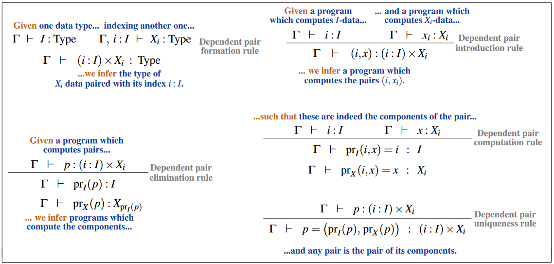
The inference rules for dependent pair types (aka “dependent sum types” or “$\Sigma$-types”):

Below in Smooth spaces - Syntactic Layer we complete this dictionary to one between dependent type theory with dependent products and toposes.