Schreiber Higher Structures
Urs Schreiber (CAS Prague & MPI Bonn)
Higher Structures in Mathematics and Physics
an introductory talk held at:
-
Meeting of Maths@CAS Brno, 2016 Nov 9-11
-
Oberwolfach Workshop 1651a, 2016 Dec. 18-23
Contents
Higher structures
The term “higher structures” is short for
mathematical structures on higher homotopy types.
We first explain what this means.
Abstract homotopy
Consider a set
Given two elements
there is the proposition
Either is equal to , or it is not.
But there may be more than one
-
way how they are equal,
-
i.e. reason that they are equal,
-
i.e. proof that they are equal.
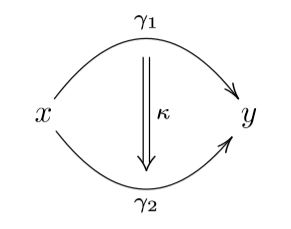
Let’s write
for one such way.
Call this a homotopy from to .
Let’s write
for the set of homotopies from to in .
Now the same reasoning applies to homotopies: given
two homotopies, there is the proposition
Either they are equal or not. But again there may be more than one way/reason/proof that exhibits their equality:
This may be called a higher homotopy.
And it keeps going this way:
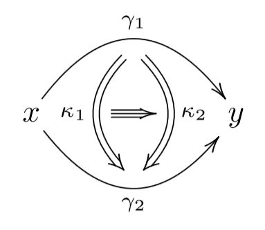
And so on.
Taking into account all these higher homotopies, the original “set” is in general richer than a set in the sense of ZFC.
To avoid clash of terminology, is called a type, or homotopy type.
One formalization of this picture is due to
- Quillen 67, K. Brown 73: “Abstract homotopy theory”
This is mostly known as the theory of “model categories”,
short for “categories of models for homotopy types”.
Another formalization of this picture is Martin-Löf type theory (Martin-Löf 73), a kind of intuitionistic constructive set theory.
That this is secretly a formalization of abstract homotopy theory was only understood more recently (Hofmann-Streicher 98, Awodey-Warren 07, Kapulkin-Lumsdaine 12)
Ever since it is also called homotopy type theory (UFP 13).
Topological homotopy
The classical model that motivated abstract homotopy theory is the homotopy theory of topological spaces.
Given two continuous functions from a topological space space to a topological space
hence given two points in the mapping space
then a homotopy between them
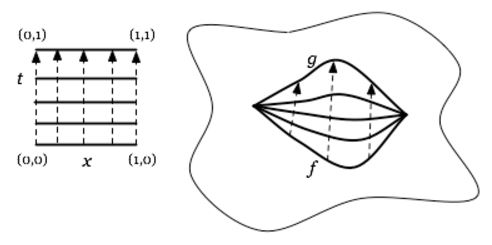
is a continuous family of continuous paths between the points
(graphics grabbed from J. Tauber here)
In this perspective topological spaces are called homotopy types.
A homotopy n-type is a space inside which there exist higher homotopies that are non-trivial up to higher homotopy only up to order .
Hence an ordinary set is equivalently a homotopy 0-type.
The rest is “higher homotopy types”.
Now a “higher structure” is a structure on higher homotopy types:
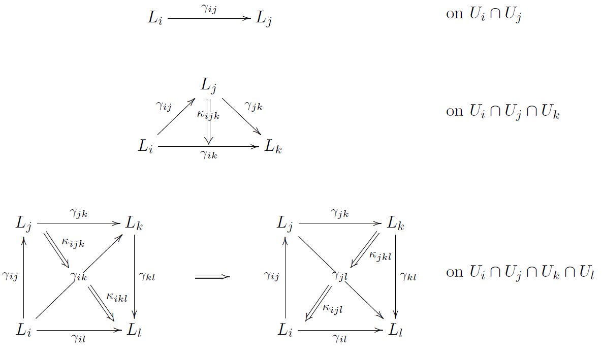
Higher structures
A mathematical structure, à la Bourbaki, is
-
a collection of sets
-
equipped with functions between them,
-
subject to equations between these functions.
Example. A group is
-
a set
-
equipped with
-
multiplication: a function
-
neutral element: a function
-
inverses: a function
-
-
such that this satisfies the equations for
A higher structure is like a Bourbakian mathematical structure but
-
replacing sets by higher homotopy types;
-
replacing equations by homotopies;
-
adding higher order homotopies to enforce coherence.
Here “coherence” is the condition that “iterated structure homotopies are unique up to homotopy”.
Example. A “first step higher group”, called a 2-group (Sinh 73, Baez-Lauda 03), is a group structure on a homotopy 1-type.
So the associativity equality is to be replaced by a choice of homotopy
called the associator.
The coherence to be imposed on this is the condition that the composite homotopy
is unique, in that the following two ways of composing associators to achieves this are related by a homotopy-of-homotopies, hence an equality (by assumption that we have just a 1-type).
This coherence condition is called the pentagon identity.
It implies coherence in the following sense:
Coherence theorem for 2-groups (MacLane 63): All homotopies of re-bracketing any expression, using the given associators, coincide.
Example (delooping 2-group)
For a discrete group, there is its classifying space denoted
or
(an Eilenberg-Mac Lane space).
For a (paracompact) topological space, then homotopy classes of continuous functions into classify -principal covering spaces of :
If happens to be an abelian group, then is a 2-group. The multiplication
is the map which classifies the tensor product of -coverings regarded as group ring-module bundles.
The existence of inverses reflects the fact that as such each -covering corresponds to a line bundle.
Higher geometric groups
Just like
-
a group may be equipped with geometry to make it a
-
or Lie group
-
or super group
-
etc.
so
-
a 2-group may be equipped with higher geometry. The result is called
-
etc.
-
and generally a group stack.
and generally
-
an infinity-group may be equipped with higher geometry. The result may be called a
(e.g. Schreiber 13)
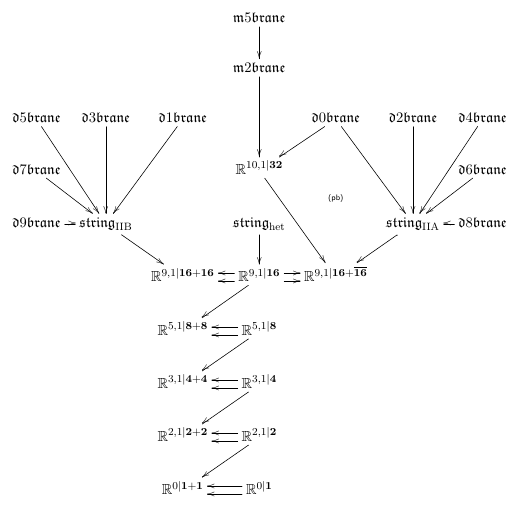
Higher principal bundles
All the usual constructions done with ordinary groups now have their higher homotopy theoretic analogs.
For instance a “parameterized group” – called a -principal bundle – is a space
equipped with a -action
over some space
such that over some open cover then there are -equivariant equivalences
over each chart .
For example the frame bundle of a smooth manifold of dimension is an general linear group-principal bundle
The higher coherent homotopy version of this definition yields
the concept of principal infinity-bundles (Nikolaus-Schreiber-Stevenson 12).
For instance a principal 2-bundle over a delooping 2-group of the form as above
is what is often called a bundle gerbe with band .
We will see examples of higher principal bundles naturally appear in the following.
Higher categorical structures
All higher homotopies are invertible, up to homotopy.
For example the inverse-up-to-homotopy of a topological homotopy
is the “reversed” map
But one may generalize further and consider non-invertible homotopies up to some order .
The result might be called “directed homotopy theory”.
But one speaks of higher categories, specifically (infinity,n)-categories.
This is more complicated than plain higher homotopy theory. The latter is the special case of (infinity,1)-categories.
More generally then:
A higher structure is a mathematical structure internal to an (infinity,n)-category.
This is also called categorification (Crane-Yetter 96, Baez-Dolan 98).
For a long time the relevant theory had been mostly missing, but now it exists (Lurie 1-).
A key application and motivation for this are extended topological quantum field theories.
Here we do not further dwell on such “directed higher structures”.
dg-Structures
Various “shadows” of higher homotopy theory are more widely familiar.
One example is chain complexes.
Consider a chain complex in non-negative degree.
Let
be two elements in degree 0, whose images in degree-0 chain homology
are equal
This means that there exists an element
in degree 1 such that
(a coboundary).
Hence every such is a reason for the equality, hence a homotopy
Next, let
be two coboundaries, both between and . Then an element
with
is a way for them to be equal
Namely this is a way for them to be equal in degree-1 chain homology
in the sense that
witnessed by
Next, an element in defines a third order homotopy
and so on.
This way each chain complex defines a homotopy type.
This is called the Dold-Kan correspondence (Dold 58, Kan 58).
Example (Poincaré lemma)
For a smooth manifold of dimension , its de Rham complex is the chain complex
of differential forms with the de Rham differential between them. If is an open ball, then there is a homotopy equivalence from the de Rham complex to
namely chain homotopies of the form
This is the statement of the Poincaré lemma. The second chain homotopy is traditionally known as the homotopy operator used in the standard proof of the Poincaré lemma.
In conclusion, there are higher mathematical structures on chain complexes.
These are often called differential graded structures, or dg-structures for short.
Here is a key example:
Higher Lie algebras
Recall the mathematical structure called a Lie algebra:
Example A Lie algebra is
-
equipped with a function
-
such that
-
skew-symmetry:
-
A higher homotopy Lie algebra structure in the homotopy theory of chain complexes, is called equivalently a
-
strong homotopy Lie algebra (the “strong” refers to the coherence)
-
L-infinity algebra (for “L”ie algebra with homotopies up to infinity)
(Lada-Stasheff 92, Lada-Markl 94).
Such a higher Lie algebra consists, first of all, of a skew-symmetric chain map
hence of a graded-skew symmetric
bilinear map that respects the differential
and which satisfies the Jacobi identity up to a specified homotopy called the Jacobiator
Then there is a coherence condition which says that the two possible ways of re-bracketing four elements are homotopic
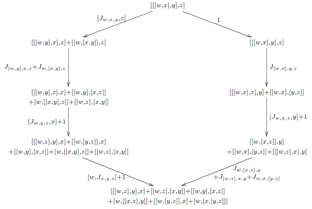
(graphics grabbed from Baez-Crans 04, p. 19)
If the chain complex is concentrated in degrees 0 and 1 then this is all the data there is. This is a Lie 2-algebra (Baez-Crans 04)
In general there is a second-order homotopy filling this diagram, which in turn satisfies its own coherence condition up to a third-order homotopy, and so on.
The following example is trivial but important for the theory.
Example. For , there is a unique higher Lie algebra structure on the chain complex
namely the one with vanishing bracket and vanishing higher homotopies. This is the line Lie (p+1)-algebra.
What are higher Lie algebras good for?
There are several answers:
-
they are equivalent to “formal moduli problems”
controlling deformation theory (Hinich 97, Pridham 07, Lurie 1-, see Doubek-Markl-Zima 07)
- in particular they they control deformation quantization via Kontsevich formality (Kontsevich 97)
-
they control closed string field theory (Zwiebach 93)
Here is yet another answer:
Higher extensions
Higher Lie algebras turn out to be the answer to the question:
What do higher Lie algebra cocycles classify?
A (p+2)-cocycle on a Lie algebra is a function
such that
-
multilinearity holds,
-
skew-symmetry holds,
-
cocycle condition: for all -tuples
Classical fact. Given a 2-cocycle it corresponds to a central extension Lie algebra extension, namely a Lie algebra structure on
given by
For this bracket the Jacobi identity is equivalently the cocycle condition on .
Fact: For then a -cocycle still defines an extension, but this is now a higher Lie algebra structure on the chain complex
whose Jacobiator and all its higher analogs are zero, except for the one of arity , which is given by .
Example. Every semisimple Lie algebra carries a Killing form pairing
and the resulting trilinear map
is a 3-cocycle.
This classifies a Lie 2-algebra extension of ,
called the string Lie 2-algebra
(Baez-Crans 03, Baez-Crans-Schreiber-Stevenson 05).
(The reason for this terminology we discuss below.)
Higher cocycles on higher Lie algebras
There are also -cocycles on higher Lie algebras .
In fact a -cocycle on a higher Lie algebra is equivalently a homomorphism of higher Lie algebras of the form
and the higher Lie algebra extension that this classifies is equivalently the homotopy fiber
(Fiorenza-Sati-Schreiber 13, prop. 3.5)
This implies that from any higher Lie algebra there emanates a “bouquet” of consecutive higher extensions
Fact. Such a higher homotopy bouquet controls the classification of super p-branes in string theory/M-theory (Fiorenza-Sati-Schreiber 13, Fiorenza-Sati-Schreiber 16).
This shows that something deep relates higher structures with physics.
We come back to this at the end.
First we now explain how higher structures appear in physics.
A higher structure at the heart of physics
Classical physics is governed by the “principle of least action”
(extremal action, really)
This is formalized in variational calculus as follows.
Let
-
be a smooth manifold of dimension ,
called the spacetime or worldvolume;
-
be a bundle (smooth map of manifolds),
called the field bundle
so that
Write
- for the jet bundle of .
This means that if
is a local coordinate chart of , then the corresponding coordinate chart of the jet bundle is
A local Lagrangian field theory is defined by a local Lagrangian density:
a -form on which is a function of the fields and some finite number of its partial derivatives
This is a horizontal differential -form on the jet bundle of .
Here the horizontal differential is the “total derivative” given in the above coordinate chart by
This defines a chain complex called the horizontal de Rham complex
Define the vertical differential on to be
This induces a chain complex of chain complexes, a double complex called the variational bicomplex
Say that the source forms are the wedge products of horizontal -forms with vertical derivatives of functions of just the fields
Euler partial integration:
Source forms are a model for the top horizontal vertical 1-forms modulo horizontal divergences:
Hence the full de Rham differential of any local Lagrangian density uniquely splits into a source-form and a horizontally exact term
This is the variational derivative.
The Euler-Lagrange equations of motion on field configurations is the partial differential equation
hence
One checks immediately that
Hence the horizontal de Rham complex continues to a longer chain complex
In fact it continues further:
This is called the Euler-Lagrange complex.
Theorem. (Vinogradov 78, Tulczyjew 80)
The Euler-Lagrange complex is locally exact. In other words, it participates in a variational version of the Poincaré lemma as above.
The Helmholtz operator on linear differential equations was found all the way back in (Helmholtz 1887).
This means for instance that
any given equation of motion
is locally a “principle of extremal action”
precisely if the Helmholtz operator annihilates it .
Hence the Euler-Lagrange complex is a higher structure at the heart of physics.
Question? What more do we gain by making it explicit this higher structure?
Surprising Answer: Many central examples of field theories may only be understood using this!
This is due to
Three well-kept secrets
| For many field theories of interest… | Example |
|---|---|
| (1) …the Lagrangian density is not globally defined. | charged particle in electromagnetic background field, WZW model, string in Kalb-Ramond field, membrane in supergravity C-field, D-brane in Kalb-Ramond field |
| (2) …the Lagrangian density is a higher connection on a higher bundle. | Wilson loop, Wilson surface, etc., |
| (3) …the field bundle is itself a higher bundle. | gauge theory such as Yang-Mills theory, Chern-Simons theory, higher gauge theory such as AKSZ sigma-model (Fiorenza-Rogers-Schreiber 11), 7d Chern-Simons theory of String 2-connection field (Fiorenza-Sati-Schreiber 14) |
| …all three of these apply. | electromagnetism with electron source fields, RR-fields with D-brane source fields (amplified in Freed 00) super p-brane with tensor multiplet such as - D-branes with Chan-Paton gauge fields - M5-brane with worldvolume gerbe (Fiorenza-Sati-Schreiber 13) |
We now explain these items in turn.
First secret: Locally variational theories
Many local Lagrangian densities of interest are not actually globally defined.
These field theories are only locally variational
(in the terminology ofAnderson-Duchamp 80, Ferraris-Palese-Winterroth 11).
This means that
-
there exists
- an open cover of the field bundle by coordinate charts
- a collection of Lagrangian densities
on each of the charts,
-
such that
-
they have a globally well defined variational derivative
in that
-
Example: charged particle
Let
-
(the “worldline”)
-
a 4d spacetime
-
the field bundle,
so that a field configuration is equivalently a smooth function
i.e. a trajectory of a particle in .
-
carrying an electromagnetic field given by a differential 2-form
called the Faraday tensor, which in a local coordinate chart
defines
an electric field and magnetic field
via
Then
-
there exists
-
an open cover
-
a collection of 1-forms
-
-
such that
and the locally defined Lagrangian density for the charged particle propagating in this background is
The Euler-Lagrange equations for this are the geodesic equations modified by the Lorentz force
Hence there is an obvious question:
When may we find a globally defined Lagrangian for the charged particle?
This is the kind of question that tools from homotopy theory naturally apply to.
We obtain the answer below,
after a closer look at the following…
Second secret: Global action functionals
A collection of chartwise defined Lagrangians is not enough data to make sense of a globally defined exponentiated action functional
Here Planck's constant coordinatizes the circle group .
Instead, making sense of this requires to choose
-
on each -fold intersection of charts
-
an order- higher homotopy
between the local Lagrangian densities:
and so on.
Such a system of local Lagrangians with higher order homotopies between them is called
a cocycle in hyper Cech cohomology
with coefficients in the horizontal Deligne complex:
Technical aside:
The statement here is that
-
Consistent assignments of phases in to field configurations are Cheeger-Simons differential characters
-
these are classified by ordinary differential cohomology,
-
which is computed by hyper Cech cohomology with coefficients in the Deligne complex.
The higher bundle underlying a local Lagrangian
Underlying any such homotopically enhanced locally variational field theory is a Cech cocycle representing an element
in the integral cohomology of the field bundle
This is given by the evident chain homomorphism
Here the chain complex
is a Lie (p+1)-group.
A cocycle as above classifies a higher principal bundle as above with higher structure group .
Fact.
The obstruction to there being a globally defined Lagrangian density is the trivialization of this higher principal bundle, hence the vanishing
of its characteristic class.
Example
In the example of the charged particle above, this is the case precisely if, in physics speak:
-
there is vanishing magnetic charge enclosed by the spacetime,
-
hence if the “-instanton number” vanishes
This is the modern incarnation of the old Dirac charge quantization phenomenon (Dirac 31).
Third secret: Higher field bundles
For exposition see: Higher field bundles for gauge fields.
Higher Noether theorem
Given a locally variational Lagrangian gerbe as above, then a symmetry is a flow
along some vertical vector field
such that it preserves the Lagrangian density in that the transformed Lagrangian density gerbe
coincides with .
In the spirit of homotopy theory, we need to choose a homotopy for each
An infinitesimal symmetry is obtained by differentiating this with respect to . This yields
where denotes the Lie derivative.
By applying
-
Euler partial integration (above)
this becomes
Here is a conserved current
in that whenever the equations of motion hold
then its horizontal differential (total divergence) vanishes.
Hence symmetries of field theories induce conserved currents.
But we could have made a different choice of homotopy
and we could have a higher order homotopy between them.
Higher Noether theorem There is an extension of the Lie algebra of symmetries by the higher Lie algebra of higher currents
(Khavkine-Schreiber, based on Fiorenza-Rogers-Schreiber 14)
Passing to chain homology, this gives ordinary Lie algebra extension.
This is the cohomological version of the Noether theorem.
(Technically aside: The conserved currents here are the “conserved currents in characteristic form” in the terminology of Olver 86, after (4.29).)
Example
Applied to Green-Schwarz sigma model for fundamental super p-branes this characterizes BPS states in supergravity. (Azcárraga-Gauntlett-Izquierdo-Townsend 89, Sati-Schreiber 15). This plays a major role in string theory.
To understand what is going on here, we now explain how these fundamental -branes work:
Example: Fundamental -branes
There are classes of examples of local variational local field theories for whose full analysis tools from higher structures are inevitable.
One such class is the generalization of the charged particle from above to higher dimensions,
called higher dimensional WZW models.
These have two kinds of applications
-
they describe the propagation of strings and generally of super p-branes in string theory/M-theory
(Henneaux-Mezincescu 85, Azcarraga-Izquierdo 95, Fiorenza-Sati-Schreiber 14
based on Green-Schwarz 84, Achúcarro-Evans-Townsend-Wiltshire 87).
-
they are argued to describe symmetry protected topological order in solid state physics
We close by discussing the archetypical case of a string propagating on a Lie group manifold.
The fundamental string in a group manifold
Let be compact simply connected simple Lie group.
Such as
-
the spin group for
-
the special unitary group for .
We consider a “charged string” propagating on , in direct analogy to the charged particle on from above.
The higher analog of the Faraday tensor now is a differential 3-form.
Recall the Lie algebra 3-cocycle from above above. By evaluating it on the Maurer-Cartan form
we obtain the closed left invariant differential form.
Pulling this back to the jet bundle along
and projecting to the horizontal component yields the “Euler-Lagrane form for the higher Lorentz force”
By the above obstruction theory we find:
there does not exist a globally defined Lagrangian density with .
Instead: there exists a bundle gerbe
such that
This is the jet bundle version (Khavkine-Schreiber) of a statement that goes back to (Gawedzki 87). For review see (Schweigert-Waldorf 07).
Theorem The higher Noether current 2-group of this sits in a homotopy fiber sequence of smooth infinity-groups
(Fiorenza-Rogers-Schreiber 13)
This identifies (Schreiber 13)
the higher Noether current group of the string
as the “smooth string 2-group” (Baez-Crans-Schreiber-Stevenson 05)
whose Lie 2-algebra is the string Lie 2-algebra from above above
Green-Schwarz anomaly cancellation
Now let
be a -principal bundle over some .
We may ask for a Lagrangian that restricts on each fiber to the one above (a “parameterized WZW model”).
Theorem (Distler-Sharpe 07, Schreiber 13) the obstruction to the parameterized WZW model on to exist is equivalently
-
a lift of to a principal 2-bundle (as above) for the string 2-group (from above)
-
vanishing of the canonical 4-class of .
If then this 4-class is
The vanishing of this class is the Green-Schwarz anomaly cancellation in heterotic string theory.
This is only the first step in a rich story.
For more on this see the lecture notes
References
Pointers to original references are given in the above text. Here we just list surveys.
-
Jim Stasheff, Higher homotopy structures, then and now, talk at Martin Markl et al. (org.) Opening conference of the program on Higher Structures in Geometry and Physics, MPI Bonn, Jan. 2016 (pdf)
-
Urs Schreiber, Higher Prequantum Geometry, (arXiv:1601.05956, v2, talk recording) chapter in Gabriel Catren, Mathieu Anel (eds.) New Spaces for Mathematics and Physics
See also
-
Higher Structures in M-Theory 2018, Durham Symposium 13-17 August 2018
-
Christian Saemann, Lectures on Higher Structures in M-Theory (arXiv:1609.09815)
Acknowledgement This note profited from suggestions by Igor Khavkine. Generally, I profited from collaborating with Igor Khavkine on higher structures in physics, please see the references in the main text above.
Last revised on August 9, 2025 at 08:43:20. See the history of this page for a list of all contributions to it.