nLab quantum adiabatic theorem
Context
Quantum systems
-
quantum algorithms:
Contents
Idea
In quantum physics, the quantum adiabatic theorem for a parameterized quantum system says the following. Under a sufficiently slow motion of the external parameters along a path in parameter space , eigenstates of the Hamiltonian at approximately evolve into eigenstates at , even if the corresponding eigenvalues change significantly. More generally, this holds for states in any part of the spectrum which stays separated from the rest of the spectrum by a gap.
For adiabatic transport along a loop, , this implies that the eigenspaces of the system are acted on by unitary operators. These are the holonomies of the Berry connection, known as Berry phases in the case of eigen-dimension 1, and as non-abelian Berry phases in the case of degenerate eigenspaces (see below).
The adiabatic parameter-action on ground states of (topologically ordered) quantum materials is one model for quantum computation: see at holonomic quantum computation and adiabatic quantum computation. If these adiabatic quantum gates depend only on the isotopy class of the parameter path, then one speaks of topological quantum computation. This is made explicit in Arovas, Schrieffer & Wilczek 1984, Freedman, Kitaev, Larsen & Wang 2003, p. 7 and Nayak, Simon, Stern, Freedman & Das Sarma 2008, §II.A.2 (p. 6); see also at braiding of anyonic defects and below.
The following graphic is meant to illustrate this general idea for the case of adiabatic transformation along the braiding of nodal points in the Brillouin torus of semi-metal quantum materials (see the discussion at braid group statistics – anyonic band nodes):
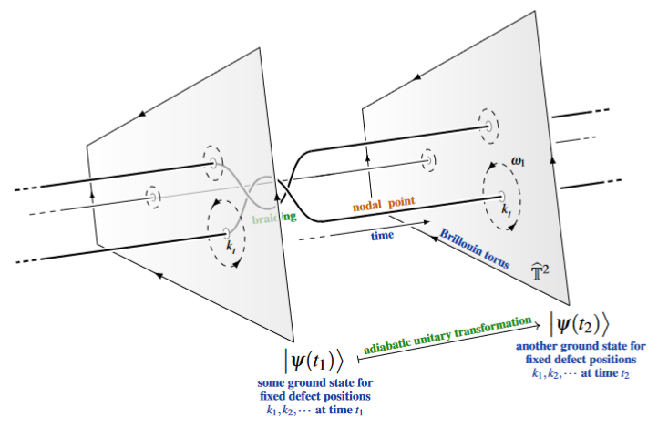
(graphics from SS22)
Statement
Preliminaries
Throughout, denotes a complex Hilbert space, its algebra of bounded operators equipped with the operator norm , and we use units with .
Adiabatic time evolution
Definition
(path of Hamiltonians)
A path of Hamiltonians is a function
to self-adjoint operators, which is twice continuously differentiable in the operator norm.
Remark
(on paths of Hamiltonians)
-
Typically such a path arises from a parameterized quantum system, namely from a family of Hamiltonians
over a smooth manifold of external parameters, by restriction along a smooth path in parameter space:
-
The restriction to bounded operators is for simplicity of exposition. Everything below generalizes to unbounded Hamiltonians which are bounded below and have a common domain , such that is as a function to bounded operators from , equipped with the graph norm? of , to (Avron, Seiler & Yaffe 1987, §2, Teufel 2003).
-
The -assumption is convenient but stronger than necessary: Kato 1950 only assumes that the first and second derivatives of the spectral projections (Def. below) are piecewise continuous.
Running through such a path in physical time means that the system evolves under the time-dependent Hamiltonian . In terms of the rescaled time parameter , the Schrödinger equation then reads as follows:
Definition
(actual time evolution)
For write
(the adiabatic parameter), and let
be the solution of
This exists, is unique, and is unitary for all , being given by the time-ordered exponential of . (It is called the dynamical transformation in Kato 1950, §2.)
The adiabatic limit is the limit , i.e. , in which the path of Hamiltonians is traversed infinitely slowly. In the rescaled time the dynamics becomes fast in this limit. For instance, if is constant and , then .
Gap condition and spectral projections
Definition
(gap condition)
A path of Hamiltonians (Def. ) satisfies the gap condition if, for all , the spectrum of decomposes into two disjoint non-empty closed subsets
such that
-
there is a contour encircling but not , which may be chosen to depend continuously on ,
-
the gap between the two parts is bounded below uniformly in :
We speak of gapped ground states if is the bottom part of the spectrum: .
In the special case that is a single eigenvalue, we say that the selected eigenstates are exactly degenerate, where the degeneracy may be 1. This is the case considered in Kato 1950.
Definition
(spectral projection)
Given a path satisfying the gap condition (Def. ), the spectral projections onto are given by the Riesz formula
We write
for their image spaces, which in the case of gapped ground states are the spaces of (quasi-)ground states.
Proposition
(properties of the spectral projections)
The spectral projections (Def. ) satisfy:
-
Each is an orthogonal projection which commutes with .
-
The function is in the operator norm.
-
The dimension of is independent of (possibly infinite).
-
The derivative is off-diagonal with respect to the decomposition , in that
and hence
Proof
The first statement is standard functional calculus (see at Riesz formula). The second follows since the resolvent is in , locally uniformly for on the contour. The third follows from the general fact that projections at operator-norm distance are unitarily equivalent, together with continuity of and connectedness of . For the last statement, differentiate to get , and then multiply this from both sides by to get . With this, . (These are equations (17) and (19) in Kato 1950, and (2.5) in Avron, Seiler & Yaffe 1987.)
Kato’s parallel transport
Definition
(Kato’s parallel transport)
Given a path of orthogonal projections, its Kato transport, called the adiabatic transformation in Kato 1950, §3, is the solution
of
Proposition
(Kato transport is unitary and intertwining)
The Kato transport (Def. ) is unitary for all , and it intertwines the projections:
Hence it restricts to unitary isomorphisms
and similarly between the orthogonal complements .
Proof
The generator is anti-self-adjoint, since , so that is unitary. For the intertwining property, consider . Then
by Prop. , so that . Kato’s original argument instead observes that satisfies the same differential equation as , and hence coincides with (Kato 1950, (20-22)). The statement about the orthogonal complements follows since , so that is also the Kato transport of .
Remark
(Kato transport as parallel transport of the Berry connection)
For , the transported vectors satisfy (using Prop. )
This says that they are covariantly constant with respect to the connection on the vector bundle whose fibers are the spaces . This is the sub-bundle of the trivial bundle with fiber cut out by the projections . Therefore the Kato transport is the parallel transport of this connection, which is known as the Berry connection:
-
If is a family of Hamiltonians over parameter space (Rem. ) satisfying the gap condition at every point, then the spaces form a vector bundle with connection . Kato transport along a loop in is the holonomy
of this connection. It depends on the loop, not just on its base point. In general it also depends on more than the homotopy class of the loop.
-
In terms of a local orthonormal frame of , the connection form has components
This is the non-abelian Berry connection (Wilczek & Zee 1984). In the case of rank 1, it is the original Berry connection (Simon 1983, Berry 1984), whose holonomy along a loop is multiplication by the Berry phase .
Remark
(transport of several spectral subspaces)
More generally, for a family of mutually orthogonal projections with , the solution of
is unitary and intertwines all of these projections simultaneously, (Kato 1950, §5). For two projections and this reduces to Def. .
General
The adiabatic theorem says that the actual dynamics follows the spectral subspaces bordered by gaps. To make this precise, one compares the actual time evolution (Def. ) with a modified evolution which preserves these spectral subspaces exactly:
Definition
(adiabatic evolution)
Given a path of Hamiltonians satisfying the gap condition (Def. ), its adiabatic evolution (Avron, Seiler & Yaffe 1987, (1.0), following Kato 1950) is the solution
of
The correction term is the generator of Kato’s parallel transport (Def. ), rescaled to the time parameter of the Schrödinger equation. It is the unique correction to which makes the evolution decouple from its complement while approximating the actual evolution as well as possible (Avron, Seiler & Yaffe 1987, §1). Accordingly, the adiabatic evolution splits into a geometric and a dynamical part:
Proposition
(structure of the adiabatic evolution)
The adiabatic evolution (Def. ) factors as
Here is the Kato transport of (Def. ), and is the solution of
which is unitary and commutes with . Consequently, is unitary and exactly intertwines the spectral projections:
Proof
Using , we have
which gives the factorization, by uniqueness of solutions. The generator of is self-adjoint, so that is unitary. It commutes with , since by Prop. and Prop. we have
Hence commutes with , and the intertwining property of follows from that of . (For a direct proof of the intertwining property see Avron, Seiler & Yaffe 1987, Lem. 2.3.)
In words: The adiabatic evolution moves the spectral subspace onto by Kato’s unitary parallel transport , while inside the spectral subspace it runs the actual dynamics . The adiabatic theorem says that this correctly describes the actual dynamics up to errors of order :
Theorem
(quantum adiabatic theorem)
Given a path of Hamiltonians (Def. ) satisfying the gap condition (Def. ), there is a constant , depending on the path but not on , such that for all :
In particular, transitions out of the spectral subspace are suppressed:
This is due to Kato 1950, (29) for the case of an exactly degenerate eigenvalue of finite multiplicity (Def. ). In the above generality it is due to Nenciu 1980, 1981 for bounded Hamiltonians, and Avron, Seiler & Yaffe 1987, Thm. 2.4 for unbounded Hamiltonians. A textbook account is in Teufel 2003.
Proof
(sketch)
The key observation is that the off-diagonal operator is a commutator with . Namely, with the resolvent , the operator
satisfies
This follows from the identity , which gives for any , together with the Riesz formula for . Moreover, is in , since is .
Now consider the wave operator , so that . The two differential equations give
This is of order 1, but it oscillates fast and may be integrated by parts:
Integrating, and using unitarity of and , yields
For the second statement, observe that , by Prop. .
This is the argument of Avron, Seiler & Yaffe 1987, §2 (wave operator (2.6), integration by parts Lemma 2.5), which in turn generalizes that of Kato 1950, §4.
Remark
(on the adiabatic theorem)
-
(size of the constant) By the above proof, the constant in Theorem is controlled by and . Roughly, it scales like
so that the adiabatic regime is , etc. Explicit bounds of this form are given in Jansen, Ruskai & Seiler 2007.
-
(higher order and exponential accuracy) The error of order comes from the boundary terms in the integration by parts. If is smooth and constant near the endpoints of the path, then repeated integration by parts shows that the transitions out of the spectral subspace at the end of the path are of order for all (Avron, Seiler & Yaffe 1987, Cor. 2.6). Under suitable analyticity assumptions they are even exponentially small in (Nenciu 1993, Hagedorn & Joye 2002, Teufel 2003).
-
(level crossings and gapless cases) If touches the rest of the spectrum at finitely many points , then the conclusion of Theorem still holds, but with in place of (Kato 1950, §4). There are versions of the adiabatic theorem without any gap condition, again without an error rate in general (Avron & Elgart 1999).
-
(on the hypotheses) The theorem concerns a fixed path, traversed ever more slowly. Heuristic “adiabaticity conditions” formulated only in terms of instantaneous matrix elements may fail (Marzlin & Sanders 2004, Amin 2009).
-
(many-body systems) For quantum lattice systems, grows with the volume, so that the above bounds become useless in the thermodynamic limit. There are versions of the adiabatic theorem with error bounds uniform in the system size, for local observables and assuming a uniform gap (Bachmann, De Roeck & Fraas 2017, 2018, Monaco & Teufel 2019, Henheik & Teufel 2022). A related approach is the quasi-adiabatic continuation of Hastings & Wen 2005 (see also Bachmann, Michalakis, Nachtergaele & Sims 2012). It provides quasi-local unitaries which map ground states along gapped paths onto each other, whereas the generator of Kato’s transport is in general not quasi-local.
For gapped ground states
We now specialize to the case of gapped ground states (Def. ). Here the dynamical part of the adiabatic evolution (Prop. ) becomes trivial up to a global phase. Hence the adiabatic theorem says that slow motion of parameters acts on ground states by the unitary parallel transport of the Berry connection.
Exactly degenerate ground states
Assume first that the ground states are exactly degenerate, so that is a single eigenvalue and
is the ground state space.
Proposition
(adiabatic evolution of degenerate ground states)
In this case the adiabatic evolution (Def. ) on ground states is
Proof
On , the generator of is , by Prop. . So acts on as multiplication by the phase , and the claim follows by Prop. . (Cf. Avron, Seiler & Yaffe 1987, p. 34.)
Combined with Theorem , this gives the main statement of Kato 1950, (29):
Corollary
(adiabatic transport of ground states)
Given a path of Hamiltonians with exactly degenerate gapped ground states, the actual time evolution on ground states satisfies, for all ,
Hence in the adiabatic limit , the time evolution acts on ground states, up to the dynamical phase , by the unitary operator
which is the parallel transport of the Berry connection (Rem. ).
Remark
(geometric nature of adiabatic ground state transport)
The unitary in Cor. has the following properties.
-
It is independent of the running time .
-
It is independent of the parameterization of the path, since the defining equation is invariant under reparameterization . So depends only on the curve of ground state spaces . For a parameterized system (Rem. ) it therefore depends only on the unparameterized path in parameter space .
-
The dynamical phase does depend on and on the parameterization, and it diverges as . But it is a global phase on all of , the same for all ground states. So it does not affect the relative phases and amplitudes between ground states.
Therefore the physically meaningful part of the adiabatic evolution of ground states is the purely geometric operation of parallel transport in the vector bundle of ground state spaces, with respect to the Berry connection (Rem. ).
In particular, adiabatic transport along a loop in parameter space, based at , maps the ground state space back to itself, acting on it by the holonomy
-
For non-degenerate ground states, , this is multiplication by the Berry phase (Simon 1983, Berry 1984).
-
For degenerate ground states, , this is a unitary matrix, the non-abelian Berry phase (Wilczek & Zee 1984). It is given by the path-ordered exponential of the non-abelian Berry connection form .
Quasi-degenerate ground states
In practice, ground state degeneracy is often only approximate. The bottom part of the spectrum is then a narrow band of width
much smaller than the gap to the rest of the spectrum. Write for the midpoint of this band. The above conclusions still hold, provided the running time is long compared to the inverse gap but short compared to the inverse splitting:
Proposition
(adiabatic evolution of quasi-degenerate ground states)
With as in Theorem , we have for all
Hence, up to a global phase, the ground states are transported by as in Cor. , within the time window
Proof
On , the generator of (Prop. ) is , where is self-adjoint with . Since the scalar part commutes with everything, we have , where . This implies . Now combine with Theorem .
Remark
(topological ground state degeneracy)
This quasi-degenerate situation is that of topologically ordered quantum materials. Here the splitting of the ground state degeneracy is exponentially small in the system size , , while the gap remains finite as (Hastings & Wen 2005). So the time window in Prop. , in which adiabatic transport of ground states is the unitary parallel transport , is wide for large systems.
Outlook: Adiabatic quantum gates
The above statements make adiabatic transport of gapped ground states a means for implementing quantum gates. The (quasi-)degenerate ground state space serves as the code space, and slowly cycling the external parameters through a loop executes the gate , up to a global phase:
-
holonomic quantum computation (Zanardi & Rasetti 1999, Pachos, Zanardi & Rasetti 1999) uses the non-abelian Berry holonomies as quantum gates. Since these depend only on the geometry of the loop, and not on its timing (Rem. ), they are insensitive to some control errors.
The achievable gates form the holonomy group . By the Ambrose-Singer theorem, this is all of if the components of the curvature of the Berry connection span the Lie algebra . Such “irreducible” connections are the generic case, and then already two generic loops generate a dense set of gates (Zanardi & Rasetti 1999, p. 96-97). Explicit loops for a universal set of gates in a concrete model are constructed in Pachos, Zanardi & Rasetti 1999.
-
topological quantum computation arises when the Berry connection is (projectively) flat. Then the holonomy depends only on the homotopy class of the loop, so that adiabatic transport constitutes a (projective) monodromy representation
of the fundamental group of parameter space. In the main example, is a configuration space of points of anyons (or of other defects, such as band nodes), is a braid group, and the monodromy representation is the braid group statistics of the anyons (Arovas, Schrieffer & Wilczek 1984, Nayak, Simon, Stern, Freedman & Das Sarma 2008, §II.A.2). The gates are then protected against all small deformations of the braiding paths. In realistic systems, flatness holds up to corrections which are exponentially small in the separation of the anyons, as for the splitting in Rem. . In this sense, holonomic quantum computation is “the (continuous) differential-geometric counterpart of the (discrete) topological QC with anyons” (Pachos, Zanardi & Rasetti 1999, p. 1).
-
This is to be distinguished from adiabatic quantum computation in the sense of Farhi, Goldstone, Gutmann & Sipser 2000. There one considers a non-degenerate ground state, and the result of the computation is encoded in the ground state of the final Hamiltonian rather than in a holonomy. The running time required by Theorem , governed by the minimal gap (Rem. ), then measures the complexity of the computation (see Albash & Lidar 2018).
Related concepts
References
General
The original formulation:
-
Max Born, Vladimir A. Fock: Beweis des Adiabatensatzes, Zeitschrift für Physik 51 (1928) 165–180 [doi:10.1007/BF01343193]
-
Tosio Kato: On the Adiabatic Theorem of Quantum Mechanics, J. Phys. Soc. Jpn. 5 (1950) 435-439 [doi:10.1143/JPSJ.5.435]
(introducing the “adiabatic transformation” , now known as Kato’s parallel transport, and proving that the actual time evolution of an isolated eigenspace approaches it, up to a dynamical phase, with error ; or in the presence of finitely many level crossings)
Textbook accounts:
-
Albert Messiah: Chapter XVII of: Quantum Mechanics, Volume II, North-Holland (1962), reprinted by Dover (1999, 2014) [ISBN:9780486409245]
-
Stefan Teufel: Adiabatic Perturbation Theory in Quantum Dynamics, Lecture Notes in Mathematics 1821, Springer (2003) [doi:10.1007/b13355]
Rigorous generalizations and refinements, including higher-order and exponentially small error estimates:
-
Gheorghe Nenciu: On the adiabatic theorem of quantum mechanics, J. Phys. A: Math. Gen. 13 (1980) L15 [doi:10.1088/0305-4470/13/2/002]
-
Gheorghe Nenciu: Adiabatic theorem and spectral concentration, Commun. Math. Phys. 82 (1981) 121-135 [doi:10.1007/BF01206948]
-
Joseph E. Avron, Ruedi Seiler, Laurence G. Yaffe: Adiabatic theorems and applications to the quantum Hall effect, Commun. Math. Phys. 110 (1987) 33-49 [doi:10.1007/BF01209015], Erratum: Commun. Math. Phys. 156 (1993) 649-650 [doi:10.1007/BF02096867]
(introducing the “adiabatic evolution” generated by for spectral subspaces bordered by gaps, and proving that it approximates the actual dynamics to order , with tunneling out of the spectral subspace smaller than any power of for smooth switching)
-
Gheorghe Nenciu: Linear adiabatic theory. Exponential estimates, Commun. Math. Phys. 152 (1993) 479-496 [doi:10.1007/BF02096616]
-
George A. Hagedorn, Alain Joye: Elementary exponential error estimates for the adiabatic approximation, J. Math. Anal. Appl. 267 (2002) 235-246 [doi:10.1006/jmaa.2001.7765]
With explicit bounds (motivated by adiabatic quantum computation):
-
Sabine Jansen, Mary Beth Ruskai, Ruedi Seiler: Bounds for the adiabatic approximation with applications to quantum computation, J. Math. Phys. 48 (2007) 102111 [arXiv:quant-ph/0603175, doi:10.1063/1.2798382]
-
Andris Ambainis, Oded Regev: An elementary proof of the quantum adiabatic theorem [arXiv:quant-ph/0411152]
On the failure of naive “adiabaticity conditions” when the rigorous hypotheses are dropped:
-
Karl-Peter Marzlin, Barry C. Sanders: Inconsistency in the Application of the Adiabatic Theorem, Phys. Rev. Lett. 93 (2004) 160408 [arXiv:quant-ph/0404022, doi:10.1103/PhysRevLett.93.160408]
-
Mohammad H. S. Amin: Consistency of the Adiabatic Theorem, Phys. Rev. Lett. 102 (2009) 220401 [arXiv:0810.4335, doi:10.1103/PhysRevLett.102.220401]
Without a spectral gap condition:
- Joseph E. Avron, Alexander Elgart: Adiabatic Theorem without a Gap Condition, Commun. Math. Phys. 203 (1999) 445-463 [arXiv:math-ph/9805022, doi:10.1007/s002200050620]
See also:
- Wikipedia: Adiabatic theorem
Holonomy and Berry phases
Interpretation of adiabatic transport as parallel transport in a vector bundle of eigenspaces over parameter space, with holonomy given by Berry phases:
-
Barry Simon: Holonomy, the Quantum Adiabatic Theorem, and Berry’s Phase, Phys. Rev. Lett. 51 (1983) 2167 [doi:10.1103/PhysRevLett.51.2167]
-
Michael Berry: Quantal phase factors accompanying adiabatic changes, Proc. Roy. Soc. Lond. A 392 (1984) 45-57 [doi:10.1098/rspa.1984.0023]
On the non-abelian generalization to degenerate eigenspaces:
-
Frank Wilczek, Anthony Zee: Appearance of Gauge Structure in Simple Dynamical Systems, Phys. Rev. Lett. 52 (1984) 2111 [doi:10.1103/PhysRevLett.52.2111]
-
Gustavo Rigolin, Gerardo Ortiz: The Adiabatic Theorem for Quantum Systems with Spectral Degeneracy, Phys. Rev. A 85 (2012) 062111 [arXiv:1111.5333, doi:10.1103/PhysRevA.85.062111]
Textbook account:
- Arno Bohm, Ali Mostafazadeh, Hiroyasu Koizumi, Qian Niu, Joseph Zwanziger: The Geometric Phase in Quantum Systems, Texts and Monographs in Physics, Springer (2003) [doi:10.1007/978-3-662-10333-3]
On adiabatic transport subject to repeated quantum measurement:
- Ludmila Viotti, Ana Laura Gramajo, Paula I. Villar, Fernando C. Lombardo, Rosario Fazio: Geometric phases along quantum trajectories, Quantum 7 (2023) 1029 [arXiv:2301.04222, doi:10.22331/q-2023-06-02-1029]
In condensed matter theory
Discussion in solid state physics and in view of gapped topological phases of matter (quantum Hall effect, topological insulators), see also Avron, Seiler & Yaffe 1987:
-
Joseph E. Avron, A. Raveh, B. Zur: Adiabatic quantum transport in multiply connected systems, Rev. Mod. Phys. 60 (1988) 873-915 [doi:10.1103/RevModPhys.60.873]
-
Matthew B. Hastings, Xiao-Gang Wen: Quasiadiabatic continuation of quantum states: The stability of topological ground-state degeneracy and emergent gauge invariance, Phys. Rev. B 72 (2005) 045141 [arXiv:cond-mat/0503554, doi:10.1103/PhysRevB.72.045141]
-
Sven Bachmann, Spyridon Michalakis, Bruno Nachtergaele, Robert Sims: Automorphic Equivalence within Gapped Phases of Quantum Lattice Systems, Commun. Math. Phys. 309 (2012) 835-871 [arXiv:1102.0842, doi:10.1007/s00220-011-1380-0]
-
Jan Carl Budich, Björn Trauzettel: From the adiabatic theorem of quantum mechanics to topological states of matter, physica status solidi (RRL) 7 1-2 (2013) 109-129 [arXiv:1210.6672, doi:10.1002/pssr.201206416]
-
David Aasen, Zhenghan Wang, Matthew B. Hastings: Adiabatic paths of Hamiltonians, symmetries of topological order, and automorphism codes, Phys. Rev. B 106 (2022) 085122 [arXiv:2203.11137, doi:10.1103/PhysRevB.106.085122]
With error bounds uniform in the system size, for gapped quantum many-body systems:
-
Sven Bachmann, Wojciech De Roeck, Martin Fraas: Adiabatic Theorem for Quantum Spin Systems, Phys. Rev. Lett. 119 (2017) 060201 [arXiv:1612.01505, doi:10.1103/PhysRevLett.119.060201]
-
Sven Bachmann, Wojciech De Roeck, Martin Fraas: The adiabatic theorem and linear response theory for extended quantum systems, Commun. Math. Phys. 361 (2018) 997-1027 [arXiv:1705.02838, doi:10.1007/s00220-018-3117-9]
-
Domenico Monaco, Stefan Teufel: Adiabatic currents for interacting fermions on a lattice, Rev. Math. Phys. 31 (2019) 1950009 [arXiv:1707.01852, doi:10.1142/S0129055X19500090]
-
Joscha Henheik, Stefan Teufel: Adiabatic theorem in the thermodynamic limit: Systems with a uniform gap, J. Math. Phys. 63 (2022) 011901 [arXiv:2012.15238, doi:10.1063/5.0051632]
Review:
- Sven Bachmann, Wojciech De Roeck, Martin Fraas: The adiabatic theorem in a quantum many-body setting, in: Analytic Trends in Mathematical Physics, Contemporary Mathematics 741 (2020) 43-58 [arXiv:1808.09985, ISBN:978-1-4704-5388-6]
For adiabatic quantum computation
On adiabatic quantum computation via non-degenerate ground states:
- Edward Farhi, Jeffrey Goldstone, Sam Gutmann, Michael Sipser: Quantum Computation by Adiabatic Evolution [arXiv:quant-ph/0001106]
Review:
- Tameem Albash, Daniel Lidar: Adiabatic quantum computation, Rev. Mod. Phys. 90 (2018) 015002 [arXiv:1611.04471, doi:10.1103/RevModPhys.90.015002]
For holonomic quantum computation
On holonomic quantum computation by non-abelian Berry phases of degenerate ground states:
-
Paolo Zanardi, Mario Rasetti: Holonomic quantum computation, Phys. Lett. A 264 (1999) 94-99 [arXiv:quant-ph/9904011, doi:10.1016/S0375-9601(99)00803-800803-8)]
-
Jiannis Pachos, Paolo Zanardi, Mario Rasetti: Non-Abelian Berry connections for quantum computation, Phys. Rev. A 61 (1999) 010305(R) [arXiv:quant-ph/9907103, doi:10.1103/PhysRevA.61.010305]
“In a sense HQC can be considered as the (continuous) differential-geometric counterpart of the (discrete) topological QC with anyons.”
For topological quantum computation
References which make explicit that the standard model of topological quantum computation by braiding of anyons is a form of adiabatic quantum computation:
-
Daniel P. Arovas, Robert Schrieffer, Frank Wilczek: Fractional Statistics and the Quantum Hall Effect, Phys. Rev. Lett. 53 (1984) 722 [doi:10.1103/PhysRevLett.53.722]
“The statistics of quasiparticles entering the quantum Hall effect are deduced from the adiabatic theorem.”
-
Daniel P. Arovas, Robert Schrieffer, Frank Wilczek, Anthony Zee: Statistical mechanics of anyons, Nuclear Physics B 251 (1985) 117-126 (reprinted in Wilczek 1990, p. 173-182) [doi:10.1016/0550-3213(85)90252-4]
-
Michael Freedman, Alexei Kitaev, Michael Larsen, Zhenghan Wang: Topological quantum computation, Bull. Amer. Math. Soc. 40 (2003) 31-38 [arXiv:quant-ph/0101025, doi:10.1090/S0273-0979-02-00964-3]
-
Chetan Nayak, Steven H. Simon, Ady Stern, Michael Freedman, Sankar Das Sarma: §II.A.2 (p. 6) of: Non-Abelian Anyons and Topological Quantum Computation, Rev. Mod. Phys. 80 (2008) 1083 [arXiv:0707.1889, doi:10.1103/RevModPhys.80.1083]
-
Meng Cheng, Victor Galitski, Sankar Das Sarma: Non-adiabatic Effects in the Braiding of Non-Abelian Anyons in Topological Superconductors, Phys. Rev. B 84 (2011) 104529 [arXiv:1106.2549, doi:10.1103/PhysRevB.84.104529]
-
Chris Cesare, Andrew J. Landahl, Dave Bacon, Steven T. Flammia, Alice Neels: Adiabatic topological quantum computing, Phys. Rev. A 92 (2015) 012336 [arXiv:1406.2690, doi:10.1103/PhysRevA.92.012336]
Last revised on November 15, 2026 at 17:46:48. See the history of this page for a list of all contributions to it.