nLab geometry of physics -- supersymmetry

$\,$

this entry is one section of “geometry of physics – supergeometry and superphysics” which is one chapter of “geometry of physics”

previous section: geometry of physics – supergeometry

next section geometry of physics – fundamental super p-branes

$\,$

In the broad sense of the word a super-symmetry is an action of a supergroup, just as an ordinary symmetry is an action of some group. In fundamental particle physics the term is used more specifically for supergroups that extend some spacetime symmetry group, and for their action on the field content of some field theory.

If, by default, spacetime is locally modeled on Minkowski spacetime (of some dimension) whose isometry group is called the Poincaré group in this dimension, then supersymmetry in the strict sense of the word is super-extension of the Poincaré group by a supergroup whose odd-graded component is a real spin representation (“Majorana representation”) of the spin group in the given dimension. The result is called the super Poincaré group for the given spacetime dimension and choice of real spin representation, the latter also being called the “number of supersymmetries”.

Just as – in the spirit of Klein geometry – one recovers Minkowski spacetime as the coset space of the Poincaré group by the Lorentz group, so the coset superspace of the super Poincaré group by the spin group-cover of the Lorentz group defines super Minkowski spacetime. A superspacetime is then a supermanifold locally modeled on super Minkowski spacetime. This is what is mostly called “superspace” in the physics literature. But other local model spacetimes may be used, such as anti-de Sitter spacetime, leading similarly to super anti-de Sitter spacetimes etc.

Just as ordinary Lie groups are usefully studied via their Lie algebras, so super Lie groups are conveniently studied via their super Lie algebras, such as the super Poincaré Lie algebra. This is hence a super Lie algebra extensions of the Poincaré Lie algebra, again with the odd-graded part identified with the given real spin representation. Such representations have the special property that they admit a $Spin$-equivariant bilinear pairing of two spinors to a vector, i.e. to an element in the Minkowski spacetime, regarded as a translation operation. This is precisely the structure that gives the odd-odd graded component of the bracket in the super Lie algebra. It is in this sense that in supersymmetry two odd spinorial transformations pair to a spacetime translation. It is noteworthy that the same bilinear spinor pairing also underlies other algebraic phenomena, such as the inner workings of twistors or the positivity relations that enter the spinorial proof of the positive energy theorem.

Since real spin representations have a comparatively rigid classification, there are algebraic constraints on supersymmetry groups in various dimensions. By a remarkable algebraic coincidence, the real spin representations in spacetime dimensions 3,4,5,6,7,10, and 11 are given by simple linear algebra over the real normed division algebras: the real numbers, the complex numbers, the quaternions and the octonions (Kugo-Townsend 82, Sudbery 84, Baez-Huerta 09, Baez-Huerta 10). (These are controled by the Fano plane, shown on the right.) This indicates some deep relation between supersymmetry and fundamental structures in mathematics (stable homotopy theory) where these algebras, and their associated Hopf fibrations, play a pivotal role in the Hopf invariant one theorem and the Adams spectral sequence.

Conversely, it turns out (theorem below) that the super Minkowski spacetimes in these dimensions are characterized as being the iterated maximal invariant central extensions of the superpoint (Huerta-Schreiber 17). This shows that supersymmetry in the special sense of spacetime supersymmetry is mathematically singled out among all supergroups. Given that supergroups themselves are mathematically singled out by Deligne's theorem on tensor categories, this shows that spacetime supersymmetry is not an ad-hoc concept and is of intrinsic interest independently of debated speculations on its realization at the (comparatively “low”) electroweak energy scale in the observable universe.

(In fact superconformal symmetry has an even more rigid classification: it exists only in dimensions 3,4,5, and 6, where it turns out to form the local super-symmetry groups appearing in the AdS-CFT correspondence.)

$\,$

$\,$

$\,$

$\,$

We start by considering the general concept of super-symmetry extensions of given ordinary symmetries:

• Supersymmetry extensions

There we find that super-extensions of spacetime symmetry are induced by real spin representations. There are several ways to get hold of real spin representations, and each of these gives one version of spacetime supersymmetry.

One way is to consider complex representations, which are easy to come by, and then try to carve out real sub-representations inside them by finding a real structure on the representation. In physics this is called the Majorana spinor construction. This we discuss in

• Real spinors as Majorana spinors

Another way to get real spin representations is to invoke some algebraic magic that allows to construct them right away. This turns out to work in spacetime dimensions 3,4,6 and 10 as well as 4,5,7 and 11 by considering $2 \times 2$ matrices with coefficients in one of the four real normed division algebras, equivalently one of the four real alternative division algebras. This we discuss in

• Real spinors via Real alternative division algebras.

Using the properties of real spin representations thus established, it is then immediate to construct spacetime supersymmetry super Lie algebras and supergroups. This we consider in

• Spacetime supersymmetry

Finally we discuss that instead of pre-describing bosonic spacetime symmetry and then asking for super-extensions of it, one may discover spacetime, spin geometry and supersymmetry all at once by a systematic mathematical process starting from just the superpoint:

• Supersymmetry from the superpoint

Supersymmetry extensions

We start by saying what it means, in generality, to have a supersymmetric extension of an ordinary symmetry. Here we are concerned with symmetry groups that are Lie groups, and we start by considering only the infinitesimal approximation, hence their Lie algebras.

To discuss super-extensions of Lie algebras, recall from geometry of physics – supergeometry the concept of super Lie algebras:

Definition

A super Lie algebra is a Lie algebra internal to the symmetric monoidal category $sVect = (Vect^{\mathbb{Z}/2}, \otimes_k, \tau^{super} )$ of super vector spaces. Hence this is

1. a super vector space $\mathfrak{g}$;

2. a homomorphism

   $$[-,-] \;\colon\; \mathfrak{g} \otimes_k \mathfrak{g} \longrightarrow \mathfrak{g}$$

   of super vector spaces (the super Lie bracket)

such that

1. the bracket is skew-symmetric in that the following diagram commutes

   $$\array{ \mathfrak{g} \otimes_k \mathfrak{g} & \overset{\tau^{super}_{\mathfrak{g},\mathfrak{g}}}{\longrightarrow} & \mathfrak{g} \otimes_k \mathfrak{g} \\ {}^{\mathllap{[-,-]}}\downarrow && \downarrow^{\mathrlap{[-,-]}} \\ \mathfrak{g} &\underset{-1}{\longrightarrow}& \mathfrak{g} }$$

   (here $\tau^{super}$ is the braiding natural isomorphism in the category of super vector spaces)

2. the Jacobi identity holds in that the following diagram commutes

   $$\array{ \mathfrak{g} \otimes_k \mathfrak{g} \otimes_k \mathfrak{g} && \overset{\tau^{super}_{\mathfrak{g}, \mathfrak{g}} \otimes_k id }{\longrightarrow} && \mathfrak{g} \otimes_k \mathfrak{g} \otimes_k \mathfrak{g} \\ & {}_{\mathllap{[-,[-,-]]} - [[-,-],-] }\searrow && \swarrow_{\mathrlap{[-,[-,-]]}} \\ && \mathfrak{g} } \,.$$

Externally this means the following:

Proposition

A super Lie algebra according to def. is equivalently

1. a $\mathbb{Z}/2$-graded vector space $\mathfrak{g}_{even} \oplus \mathfrak{g}_{odd}$;

2. equipped with a bilinear map (the super Lie bracket)

   $$[-,-] : \mathfrak{g}\otimes_k \mathfrak{g} \to \mathfrak{g}$$

   which is graded skew-symmetric: for $x,y \in \mathfrak{g}$ two elements of homogeneous degree $\sigma_x$, $\sigma_y$, respectively, then

   $$[x,y] = -(-1)^{\sigma_x \sigma_y} [y,x] \,,$$

3. that satisfies the $\mathbb{Z}/2$-graded Jacobi identity in that for any three elements $x,y,z \in \mathfrak{g}$ of homogeneous super-degree $\sigma_x,\sigma_y,\sigma_z\in \mathbb{Z}_2$ then

   $$[x, [y, z]] = [[x,y],z] + (-1)^{\sigma_x \cdot \sigma_y} [y, [x,z]] \,.$$

A homomorphism of super Lie algebras is a homomorphisms of the underlying super vector spaces which preserves the Lie bracket. We write

$$sLieAlg$$

for the resulting category of super Lie algebras.

Some obvious but important classes of examples are the following:

Example

Every $\mathbb{Z}/2$-graded vector space $V$ becomes a super Lie algebra (def. , prop. ) by taking the super Lie bracket to be the zero map

$$[-,-] = 0 \,.$$

These may be called the “abelian” super Lie algebras.

Example

Every ordinary Lie algebras becomes a super Lie algebra (def. , prop. ) concentrated in even degrees. This constitutes a fully faithful functor

$$LieAlg \hookrightarrow sLieAlg \,.$$

which is a coreflective subcategory inclusion in that it has a left adjoint

$$LieAlg \underoverset {\underset{ \overset{ \rightsquigarrow}{(-)} }{\longleftarrow}} {\hookrightarrow} {\phantom{AA}\bot\phantom{AA}} sLieAlg$$

given on the underlying super vector spaces by restriction to the even graded part

$$\overset{\rightsquigarrow}{\mathfrak{s}} = \mathfrak{s}_{even} \,.$$

Using this we may finally say what a super-extension is supposed to be:

Definition

Given an ordinary Lie algebra $\mathfrak{g}$, then a super-extension of $\mathfrak{g}$ is super Lie algebra $\mathfrak{s}$ (def. , prop. ) equipped with a monomorphism of the form

$$i \;\colon\; \mathfrak{g} \hookrightarrow \mathfrak{s}$$

(where $\mathfrak{g}$ is regarded as a super Lie algebra according to example )

such that this is an isomorphism on the even part (example )

$$\overset{\rightsquigarrow}{i} \;\colon\; \mathfrak{g} \overset{\simeq}{\longrightarrow} \mathfrak{s}_{even} \,.$$

We now make explicit structure involved in super-extensions of Lie algebras:

Proposition

Given an ordinary Lie algebra $\mathfrak{g}$, then a choice of super-extension $\mathfrak{g} \hookrightarrow \mathfrak{s}$ according to def. is equivalently the following data:

1. a vector space $S$;

2. a Lie action of $\mathfrak{g}$ on $S$, hence a Lie algebra homomorphism

   $$\rho_{(-)} : \mathfrak{g} \longrightarrow \mathfrak{gl}(S)$$

   from $\mathfrak{g}$ to the endomorphism Lie algebra of $S$;

3. a symmetric bilinear map

   $$(-,-) \;\colon\; S \otimes_k S \longrightarrow \mathfrak{g}$$

such that

1. the pairing is $\mathfrak{g}$-equivariant in that for all $t \in \mathfrak{g}$ then

   $$\rho_{t}(-,-) = (\rho_t(-),(-)) + (-,\rho_t(-))$$

2. the pairing satisfies

   $$\rho_{(\phi,\phi)}(\phi) = 0$$

   for all $\phi \in S$.

Proof

By definition of super-extension, the underlying super vector space of $\mathfrak{s}$ is necessarily of the form

$$\mathfrak{s}_{even} = \underset{\mathfrak{s}_{even}}{\underbrace{\mathfrak{g}}} \oplus \underset{\mathfrak{s}_{odd}}{\underbrace{S}}$$

for some vector space $S$.

Moreover the super Lie bracket on $\mathfrak{s}$ restricts to that of $\mathfrak{g}$ when restricted to $\mathfrak{g} \otimes_{k}\mathfrak{g}$ and otherwise constitutes

1. a bilinear map

   $$\rho_{(-)}(-) \coloneqq [-,-]\vert_{\mathfrak{s}_{even}\oplus \mathfrak{s}_{odd}} \;\colon\; \mathfrak{g} \otimes_k S \longrightarrow S$$

2. a symmetric bilinear map

   $$(-,-) \coloneqq [-,-]\vert_{\mathfrak{s}_{odd} \oplus \mathfrak{s}_{odd}} \;\colon\; S \otimes_k S \longrightarrow \mathfrak{g} \,.$$

This yields the claimed structure. The claimed properties of these linear maps are now just a restatement of the super-Jacobi identity in terms of this data:

1. The restriction of the super Jacobi identity of $\mathfrak{s}$ to $\mathfrak{s}_{even} \otimes_k \mathfrak{s}_{even} \otimes_k \mathfrak{s}_{even}$ is equivalently the Jacobi identity on $\mathfrak{g}$ and hence is no new constraint.

2. The restriction of the super Jacobi identity of $\mathfrak{s}$ to $\mathfrak{s}_{even} \otimes_k \mathfrak{s}_{even} \otimes_k \mathfrak{s}_{odd}$ says that for $t_1,t_2 \in \mathfrak{g}$ and $\phi \in S$ then

   $$\rho_{t_1}( \rho_{t_2}(\phi) ) = \rho_{[t_1,t_2]}(\phi) + \rho_{t_1}( \rho_{t_2}(\phi) ) \,.$$

   This is equivalent to

   $$\rho_{t_1} \circ \rho_{t_2} - \rho_{t_2} \circ \rho_{t_1} = \rho_{[t_1,t_2]}$$

   which means equivalently that $\rho_{(-)}$ is a Lie algebra homomorphism from $\mathfrak{g}$ to the endomorphism Lie algebra of $S$, hence that it is a Lie algebra representation of $\mathfrak{g}$ on $S$.

3. The restriction of the super Jacobi identity of $\mathfrak{s}$ to $\mathfrak{s}_{even} \otimes_k \mathfrak{s}_{odd} \otimes_k \mathfrak{s}_{odd}$ says that for $t \in \mathfrak{g}$ and $\phi,\psi \in S$ then

   $$\rho_{t}(\phi,\psi) = (\rho_t(\phi), \psi) + (\phi, \rho_t(\psi)) \,.$$

   This is exactly the claimed $\mathfrak{g}$-equivariance of the pairing.

4. The restriction of the super Jacobi identity of $\mathfrak{s}$ to $\mathfrak{s}_{odd} \otimes_k \mathfrak{s}_{odd} \otimes_k \mathfrak{s}_{odd}$ implies that for all $\psi \in S$ that

   $$[\psi,(\psi,\psi)] = [ (\psi,\psi), \psi ] - [\psi, (\psi, \psi)]$$

   and hence in particular that

   $$[(\psi,\psi),\psi] = \rho_{(\psi,\psi)}(\psi) = 0 \,.$$

   Therefore it only remains to show that this special case is in fact equivalent to the full odd-odd-odd super Jacobi identity. This follows by polarization: First insert $\psi = \phi_1 + \phi_2$ into the above cubic condition to obtain a quadratic condition, then polarize once more in $\phi_2$.

Example

(trivial super extension)

Given an ordinary Lie algebra $\mathfrak{g}$, then for every choice of vector space $V$ there is the trivial super extension (def. ) of $\mathfrak{g}$, with underlying vector space

$$\mathfrak{s} \coloneqq \mathfrak{g} \oplus S$$

and with both the action and the pairing (via prop. ) trivial:

$$\rho = 0$$

and

$$(-,-) = 0 \,.$$

The key example of interest now is going to be this:

Example

(super Poincaré super Lie algebra)

For $d \in \mathbb{N}$, a super extension (def. ) of the Poincaré Lie algebra $\mathfrak{iso}(\mathbb{R}^{d-1,1})$ (recalled as def. below) which is non-trivial (def. ) is obtained from the following data:

1. a Lie algebra representation $\rho$ of $\mathfrak{so}(d-1,1)$ on some real vector space $S$;

2. an $\mathfrak{so}$-equivariant symmetric $\mathbb{R}$-bilinear pairiing $(-,-) \colon S \otimes_k S \to \mathbb{R}^{d-1,1}$

It turns out that data as in example is given for $\rho$ the Lie algebra version of a real spin representation of the spin group $Spin(d-1,1)$ (this is prop. below). These we introduce and discuss now in Real spin representations.

The super-extensions of the Poincaré Lie algebra induced by real spin representations are called super Poincaré Lie algebras (def. ) below. These are the standard supersymmetry algebras in the physics literature.

But beware that there are more (“exotic”) super-extensions of the Poincaré Lie algebra than the “standard supersymmetry” super Poincaré Lie algebra from example : (The following example uses facts which we establish further below, the reader may want to skip this now and come back to it later.)

Example

(an exotic super-extension of the Poincaré Lie algebra)

Let $d \in \{3,4,6,10\}$ and let $S \in Rep_{\mathbb{R}}(Spin(d-1,1))$ be an irreducible real spin representation in that dimension. Let $(-,-) \colon S \otimes S \to \mathbb{R}^{d-1,1}$ be the symmetric spinor pairing as in example , but let the action on $S$ via the even-odd super-bracket not be the Spin-action of $\mathfrak{so}$, but the Clifford algebra action

$$\Gamma(-) \;\colon \; \mathbb{R}^{d-1,1} \longrightarrow End(S) \,.$$

of $\mathbb{R}^{d-1,1}$. Then the condition

$$\Gamma(\psi,\psi)(\psi) = 0$$

from prop. does hold: this turns out to be equivalent to the Green-Schwarz superstring cocycle condition in these dimensions, here in its incarnation as the “3-$\psi$ rule” of Schray 96, see Baez-Huerta 09, theorem 10.

Now $\Gamma(-)$ thus defined is clearly not a Lie algebra action and hence fails one of the other conditions in prop. , but this is readily fixed: take $S \coloneqq S_+ \oplus S_-$ to be the direct sum of two copies of the Majorana spinor representation and take $\Gamma(-)$ to map as before, but from $S_+$ to $S_-$, acting as zero on $S_-$. This forces the commutator of endomorphisms in the image of $\Gamma$ to vanish, and hence makes $\Gamma(-)$ a Lie algebra action of the abelian Lie algebra $\mathbb{R}^{d-1,1}$. Hence we get an “exotic” super-extension of the Poincaré Lie algebra.

Remark

By prop. the data in example is sufficient for producing super-extensions (in the sense of def. ) of Poincaré Lie algebras, namely the super Poincaré Lie algebras. It is however not necessary: example is a super-extension in the sense of def. of the Poincaré Lie algebra which is not a super Poincaré Lie algebra in the standard sense of example .

One may add further natural conditions on the super-extension in order to narrow down to the super Poincaré super Lie algebras:

1. From the assumption alone that $S$ is a spin representation and using that the $Spin$-equivariant pairing has to take irreducible representations to irreducible representations, one may in some dimensions already deduce that the pairing has to land in $\mathbb{R}^{d} \hookrightarrow \mathfrak{iso}(\mathbb{R}^{d-1,1})$. For $d = 4$ and $S$ the irreducible Majorana representation this is done in Varadarajan 04, section 3.2.

2. One may appeal to the Haag-Łopuszański-Sohnius theorem. This does rule out exotic super-extensions, by imposing the additional condition that $P_a P^a$ remains a Casimir operator after super-extension, and more conditions. These conditions are well motivated from the expected symmetry-behaviour of S-matrices in field theory.

Below in supersymmetry from the superpoint we discuss a more fundamental statement: The super Poincaré Lie algebras at least in certain dimensions are singled out from a different perspective: they are precisely the result of iterative maximal invariant central extensions of the superpoint.

Real spin representations

By example we want a real spin representation in order to construct a spacetime supersymmetry super Lie algebra. There are different ways to get hold of real spin representations.

One way is to first consider complex representations, which are easy to come by, and then try to carve out real sub-representations inside them by finding a real structure on the representation. In physics this is called the Majorana spinor construction. This we discuss in

• Real spinors as Majorana spinors

Another way to get real spin representations is to invoke some algebraic magic that allows to construct them right away. This turns out to work in spacetime dimensions 3,4,6 and 10 as well as 4,5,7 and 11 by considering $2 \times 2$ matrices with coefficients in one of the four real normed division algebras, equivalently one of the four real alternative division algebras. This we discuss in

• Real spinors via Real alternative division algebras.

Real spinors as Majorana spinors

We will discuss the following concept, the ingredients of which we explain in the following

Definition

For $d \in \mathbb{N}$, write $Spin(d-1,1)$ for the spin group (def. ) double cover (prop. ) of the proper orthochronous Lorentz group (def. ), let

$$\rho \colon Spin(d-1,1) \longrightarrow GL_{\mathbb{C}}(V)$$

be a unitary linear representation of $Spin(d-1,1)$ on some complex vector space $V$.

Then $\rho$ is called

• a Majorana representation if it admits a real structure $J$ (def. );

  an element $\psi \in V$ is then called a real spinor if $J(\psi) = \psi$.

• a symplectic Majorana representation if it admits a quaternionic structure $J$ (def. )

  In this case $\tilde J \coloneqq \left( \array{ 0 & J \\ -J & 0 }\right)$ is a real structure on $V \oplus V$ and in this way also symplectic Majorana spinors are regarded as a real spin representation.

We discuss this now in components (i.e. in terms of choices of linear bases), using standard notation and conventions from the physics literature (e.g. Castellani-D’Auria-Fré), but taking care to exhibit the abstract concept of real representations.

Below we work out the following:

Proposition

Let $V = \mathbb{R}^{d-1,1}$ be Minkowski spacetime of some dimension $d$.

The following table lists the irreducible real spin representations of $Spin(V)$.

$d$	$Spin(d-1,1)$	minimal real spin representation $S$	$dim_{\mathbb{R}} S\;\;$	$V$ in terms of $S^\ast$	supergravity
1	$\mathbb{Z}_2$	$S$ real	1	$V \simeq (S^\ast)^{\otimes}^2$
2	$\mathbb{R}^{\gt 0} \times \mathbb{Z}_2$	$S^+, S^-$ real	1	$V \simeq ({S^+}^\ast)^{\otimes^2} \oplus ({S^-}^\ast)^{\otimes 2}$
3	$SL(2,\mathbb{R})$	$S$ real	2	$V \simeq Sym^2 S^\ast$
4	$SL(2,\mathbb{C})$	$S_{\mathbb{C}} \simeq S' \oplus S''$	4	$V_{\mathbb{C}} \simeq {S'}^\ast \oplus {S''}^\ast$	d=4 N=1 supergravity
5	$Sp(1,1)$	$S_{\mathbb{C}} \simeq S_0 \otimes_{\mathbb{C}} W$	8	$\wedge^2 S_0^\ast \simeq \mathbb{C} \oplus V_{\mathbb{C}}$
6	SL(2,H)	$S^\pm_{\mathbb{C}} \simeq S_0^\pm \otimes_{\mathbb{C}} W$	8	$V_{\mathbb{C}} \simeq \wedge^2 {S_0^+}^\ast \simeq (\wedge^2 {S_0^-}^\ast)^\ast$
7		$S_{\mathbb{C}} \simeq S_0 \otimes_{\mathbb{C}} W$	16	$\wedge^2 S_0^\ast \simeq V_{\mathbb{C}} \oplus \wedge^2 V_{\mathbb{C}}$
8		$S_{\mathbb{C}} \simeq S^\prime \oplus S^{\prime\prime}$	16	${S'}^\ast {S''}^\ast \simeq V_{\mathbb{C}} \oplus \wedge^3 V_{\mathbb{C}}$
9		$S$ real	16	$Sym^2 S^\ast \simeq \mathbb{R} \oplus V \wedge^4 V$
10		$S^+ , S^-$ real	16	$Sym^2(S^\pm)^\ast \simeq V \oplus \wedge_\pm^5 V$	type II supergravity
11		$S$ real	32	$Sym^2 S^\ast \simeq V \oplus \wedge^2 V \oplus \wedge^5 V$	11-dimensional supergravity

Here $W$ is the 2-dimensional complex vector space on which the quaternions naturally act.

(table taken from Freed 99, page 48)

Spin

We recall the basics of Minkowski spacetimes $\mathbb{R}^{d-1,1}$, their Clifford algebras and spin groups.

Definition

For $d \in \mathbb{N}$, we write $\mathbb{R}^{d-1,1}$ for the real vector space $\mathbb{R}^{d}$ equipped with the quadratic form $\eta$ of signature

$$\eta = diag(+1, \cdots, +1, - 1) \,.$$

We write the standard coordinates on $\mathbb{R}^{d-1,1}$

$$(x_0, x_1, x_2, \cdots, x_{d-1})$$

with $x_0$ the coordinate along the timelike direction: for $v = v^a x_a \in \mathbb{R}^{d-1,1}$ any vector, then

$$\eta(v,v) = -(v^0)^2 + \underoverset{i = 1}{d-1}{\sum} (v^{i})^2 \,.$$

Definition

For $d \in \mathbb{N}$, write

$$O(d-1,1) \hookrightarrow GL(\mathbb{R}^d)$$

for the subgroup of the general linear group on those linear maps $A$ which preserve this bilinear form on Minkowski spacetime (def ), in that

$$\eta(A(-),A(-)) = \eta(-,-) \,.$$

This is the Lorentz group in dimension $d$.

The elements in the Lorentz group in the image of the special orthogonal group $SO(d-1) \hookrightarrow O(d-1,1)$ are rotations in space. The further elements in the special Lorentz group $SO(d-1,1)$, which mathematically are “hyperbolic rotations” in a space-time plane, are called boosts in physics.

One distinguishes the following further subgroups of the Lorentz group $O(d-1,1)$:

• the proper Lorentz group

  $$SO(d-1,1) \hookrightarrow O(d-1,1)$$

  is the subgroup of elements which have determinant +1 (as elements $SO(d-1,1)\hookrightarrow GL(d)$ of the general linear group);

• the proper orthochronous (or restricted) Lorentz group

  $$SO^+(d-1,1) \hookrightarrow SO(d-1,1)$$

  is the further subgroup of elements $A$ which preserve the time orientation of vectors $v$ in that $(v^0 \gt 0) \Rightarrow ((A v)^0 \gt 0)$.

Proposition

As a smooth manifold, the Lorentz group $O(d-1,1)$ (def. ) has four connected components. The connected component of the identity is the proper orthochronous Lorentz group $SO^+(3,1)$ (def. ). The other three components are

1. $SO^+(d-1,1)\cdot P$

2. $SO^+(d-1,1)\cdot T$

3. $SO^+(d-1,1)\cdot P T$,

where, as matrices,

$$P \coloneqq diag(1,-1,-1, \cdots, -1)$$

is the operation of point reflection at the origin in space, where

$$T \coloneqq diag(-1,1,1, \cdots, 1)$$

is the operation of reflection in time and hence where

$$P T = T P = diag(-1,-1, \cdots, -1)$$

is point reflection in spacetime.

The following concept of the Clifford algebra (def. ) of Minkowski spacetime encodes the structure of the inner product space $\mathbb{R}^{d-1,1}$ in terms of algebraic operation (“geometric algebra”), such that the action of the Lorentz group becomes represented by a conjugation action (example below). In particular this means that every element of the proper orthochronous Lorentz group may be “split in half” to yield a double cover: the spin group (def. below).

Definition

For $d \in \mathbb{N}$, we write

$$Cl(\mathbb{R}^{d-1,1})$$

for the $\mathbb{Z}/2$-graded associative algebra over $\mathbb{R}$ which is generated from $d$ generators $\{\Gamma_0, \Gamma_1, \Gamma_2, \cdots, \Gamma_{d-1}\}$ in odd degree (“Clifford generators”), subject to the relation

$$\Gamma_{a} \Gamma_b + \Gamma_b \Gamma_a = - 2\eta_{a b}$$

where $\eta$ is the inner product of Minkowski spacetime as in def. .

These relations say equivalently that

$$\begin{aligned} & \Gamma_0^2 = +1 \\ & \Gamma_i^2 = -1 \;\; \text{for}\; i \in \{1,\cdots, d-1\} \\ & \Gamma_a \Gamma_b = - \Gamma_b \Gamma_a \;\;\; \text{for}\; a \neq b \end{aligned} \,.$$

We write

$$\Gamma_{a_1 \cdots a_p} \;\coloneqq\; \frac{1}{p!} \underset{{permutations \atop \sigma}}{\sum} (-1)^{\vert \sigma\vert } \Gamma_{a_{\sigma(1)}} \cdots \Gamma_{a_{\sigma(p)}}$$

for the antisymmetrized product of $p$ Clifford generators. In particular, if all the $a_i$ are pairwise distinct, then this is simply the plain product of generators

$$\Gamma_{a_1 \cdots a_n} = \Gamma_{a_1} \cdots \Gamma_{a_n} \;\;\; \text{if} \; \underset{i,j}{\forall} (a_i \neq a_j) \,.$$

Finally, write

$$\overline{(-)} \;\colon\; Cl(\mathbb{R}^{d-1,1}) \longrightarrow Cl(\mathbb{R}^{d-1,1})$$

for the algebra anti-automorphism given by

$$\overline{\Gamma_a} \coloneqq \Gamma_a$$

$$\overline{\Gamma_a \Gamma_b} \coloneqq \Gamma_b \Gamma_a \,.$$

Remark

By construction, the vector space of linear combinations of the generators in a Clifford algebra $Cl(\mathbb{R}^{d-1,1})$ (def. ) is canonically identified with Minkowski spacetime $\mathbb{R}^{d-1,1}$ (def. )

$$\widehat{(-)} \;\colon\; \mathbb{R}^{d-1,1} \hookrightarrow Cl(\mathbb{R}^{d-1,1})$$

via

$$x_a \mapsto \Gamma_a \,,$$

hence via

$$v = v^a x_x \mapsto \hat v = v^a \Gamma_a \,,$$

such that the defining quadratic form on $\mathbb{R}^{d-1,1}$ is identified with the anti-commutator in the Clifford algebra

$$\eta(v_1,v_2) = -\tfrac{1}{2}( \hat v_1 \hat v_2 + \hat v_2 \hat v_1) \,,$$

where on the right we are, in turn, identifying $\mathbb{R}$ with the linear span of the unit in $Cl(\mathbb{R}^{d-1,1})$.

The key point of the Clifford algebra (def. ) is that it realizes spacetime reflections, rotations and boosts via conjugation actions:

Example

For $d \in \mathbb{N}$ and $\mathbb{R}^{d-1,1}$ the Minkowski spacetime of def. , let $v \in \mathbb{R}^{d-1,1}$ be any vector, regarded as an element $\hat v \in Cl(\mathbb{R}^{d-1,1})$ via remark .

Then

1. the conjugation action $\hat v \mapsto -\Gamma_a^{-1} \hat v \Gamma_a$ of a single Clifford generator $\Gamma_a$ on $\hat v$ sends $v$ to its

reflection at the hyperplane $x_a = 0$;

1. the conjugation action

   $$\hat v \mapsto \exp(- \tfrac{\alpha}{2} \Gamma_{a b}) \hat v \exp(\tfrac{\alpha}{2} \Gamma_{a b})$$

   sends $v$ to the result of rotating it in the $(a,b)$-plane through an angle $\alpha$.

Proof

This is immediate by inspection:

For the first statement observe that conjugating the Clifford generator $\Gamma_b$ with $\Gamma_a$ yields $\Gamma_b$ up to a sign, depending on whether $a = b$ or not:

$$- \Gamma_a^{-1} \Gamma_b \Gamma_a = \left\{ \array{ -\Gamma_b & \vert \text{if}\, a = b \\ \Gamma_b & \vert \text{otherwise} } \right. \,.$$

Therefore for $hat v = v^b \Gamma_b$ then $\Gamma_a^{-1} \hat v \Gamma_a$ is the result of multiplying the $a$-component of $v$ by $-1$.

For the second statement, observe that

$$-\tfrac{1}{2}[\Gamma_{a b}, \Gamma_c] = \Gamma_a \eta_{b c} - \Gamma_b \eta_{a c} \,.$$

This is the canonical action of the Lorentzian special orthogonal Lie algebra $\mathfrak{so}(d-1,1)$. Hence

$$\exp(-\tfrac{\alpha}{2} \Gamma_{ab}) \hat v \exp(\tfrac{\alpha}{2} \Gamma_{ab}) = \exp(\tfrac{1}{2}[\Gamma_{a b}, -])(\hat v)$$

is the rotation action as claimed.

Remark

Since the reflections, rotations and boosts in example are given by conjugation actions, there is a crucial ambiguity in the Clifford elements that induce them:

1. the conjugation action by $\Gamma_a$ coincides precisely with the conjugation action by $-\Gamma_a$;

2. the conjugation action by $\exp(\tfrac{\alpha}{4} \Gamma_{a b})$ coincides precisely with the conjugation action by $-\exp(\tfrac{\alpha}{2}\Gamma_{a b})$.

Definition

For $d \in \mathbb{N}$, the spin group $Spin(d-1,1)$ is the group of even graded elements of the Clifford algebra $Cl(\mathbb{R}^{d-1,1})$ (def. ) which are unitary with respect to the conjugation operation $\overline{(-)}$ from def. :

$$Spin(d-1,1) \;\coloneqq\; \left\{ A \in Cl(\mathbb{R}^{d-1,1})_{even} \;\vert\; \overline{A} A = 1 \right\} \,.$$

Proposition

The function

$$Spin(d-1,1) \longrightarrow GL(\mathbb{R}^{d-1,1})$$

from the spin group (def. ) to the general linear group in $d$-dimensions given by sending $A \in Spin(d-1,1) \hookrightarrow Cl(\mathbb{R}^{d-1,1})$ to the conjugation action

$$\overline{A}(-) A$$

(via the identification of Minkowski spacetime as the subspace of the Clifford algebra containing the linear combinations of the generators, according to remark )

is

1. a group homomorphism onto the proper orthochronous Lorentz group (def. ):

   $$Spin(d-1,1) \longrightarrow SO^+(d-1,1)$$

2. exhibiting a $\mathbb{Z}/2$-central extension.

Proof

That the function is a group homomorphism into the general linear group, hence that it acts by linear transformations on the generators follows by using that it clearly lands in automorphisms of the Clifford algebra.

That the function lands in the Lorentz group $O(d-1,1) \hookrightarrow GL(d)$ follows from remark :

$$\begin{aligned} \eta(\overline{A}v_1A , \overline{A} v_2 A) &= \tfrac{1}{2} \left( \left(\overline{A} \hat v_1 A\right) \left(\overline{A}\hat v_2 A\right) + \left(\overline{A} \hat v_2 A\right) \left(\overline{A} \hat v_1 A\right) \right) \\ & = \tfrac{1}{2} \left( \overline{A}(\hat v_1 \hat v_2 + \hat v_2 \hat v_1) A \right) \\ & = \overline{A} A \tfrac{1}{2}\left( \hat v_1 \hat v_2 + \hat v_2 \hat v_1\right) \\ & = \eta(v_1, v_2) \end{aligned} \,.$$

That it moreover lands in the proper Lorentz group $SO(d-1,1)$ follows from observing (example ) that every reflection is given by the conjugation action by a linear combination of generators, which are excluded from the group $Spin(d-1,1)$ (as that is defined to be in the even subalgebra).

To see that the homomorphism is surjective, use that all elements of $SO(d-1,1)$ are products of rotations in hyperplanes. If a hyperplane is spanned by the bivector $(\omega^{a b})$, then such a rotation is given, via example by the conjugation action by

$$\exp(\tfrac{\alpha}{2} \omega^{a b}\Gamma_{a b})$$

for some $\alpha$, hence is in the image.

That the kernel is $\mathbb{Z}/2$ is clear from the fact that the only even Clifford elements which commute with all vectors are the multiples $a \in \mathbb{R} \hookrightarrow Cl(\mathbb{R}^{d-1,1})$ of the identity. For these $\overline{a} = a$ and hence the condition $\overline{a} a = 1$ is equivalent to $a^2 = 1$. It is clear that these two elements $\{+1,-1\}$ are in the center of $Spin(d-1,1)$. This kernel reflects the ambiguity from remark .

Real structure on Unitary representations

We are interested in spin representations on real vector spaces. It turns out to be useful to obtain these from unitary representations on complex vector spaces by equipping these with real structure. In any case this is the approach used in much of the (physics) literature (with the real structure usually not made explicit, but phrased in terms of (symplectic) Majorana conditions).

Hence for reference, we here recollect the basics of the concept of unitary representations equipped with real structure.

All vector spaces in the following are taken to be finite dimensional vector spaces.

Definition

Let $V$ be a complex vector space. A real structure or quaternionic structure on $V$ is a real-linear map

$$\phi \;\colon\; V \longrightarrow V$$

such that

1. $\phi$ is conjugate linear, in that $\phi(\lambda v) = \overline{\lambda} \phi(v)$ for all $\lambda \in \mathbb{C}$, $v \in V$;

2. $\phi^2 = \left\{ \array{ +id & \text{for real structure} \\ -id & \text{for quaternionic structure} } \right.$

Remark

A real structure $\phi$, def. , on a complex vector space $V$ corresponds to a choice of complex linear isomorphism

$$V \simeq \mathbb{C} \otimes_{\mathbb{R}} V_+$$

of $V$ with the complexification of a real vector space $V_+$, namely the eigenspace of $\phi$ for eigenvalue +1, while $V_- \coloneqq i V_+$ is the eigenspace of eigenvalue -1.

A quaternionic structure, def. , on $V$ gives it the structure of a left module over the quaternions (def. ) extending the underlying structure of a module over the complex numbers. Namely let

1. $I \coloneqq i(-) \colon V \to V$ be the operation of multiplying with $i \in \mathbb{C}$

2. $J \coloneqq \phi \colon V \to V$ be the given endomorphisms,

3. $K \coloneqq I \circ J$ their composite,

then the conjugate complex linearity of $\phi$ implies that

$$J \circ I = - I \circ J$$

and hence with $J^2 = -1$ and $I^2 = -1$ this means that $I$, $J$ and $K$ act like the imaginary quaternions.

Definition

Let $G$ be a Lie group, let $V$ be a complex vector space and let

$$\rho \;\colon\; G \longrightarrow GL_{\mathbb{C}}(V)$$

be a complex linear representation of $G$ on $V$, hence a group homomorphism form $G$ to the general linear group of $V$ over $\mathbb{C}$.

Then a real structure or quaternionic structure on $(V,\rho)$ is a real or complex structure, respectively, $\phi$ on $V$ (def. ) such that $\phi$ is $G$-invariant under $\rho$, i.e. such that for all $g \in G$ then

$$\phi \circ \rho(g) = \rho(g) \circ \phi \,.$$

We will be interested in complex finite dimensional vector spaces equipped with hermitian forms, i.e. finite-dimensional complex Hilbert spaces:

Definition

A hermitian form (or symmetric complex sesquilinear form) $\langle -,-\rangle$ on a complex vector space $V$ is a real bilinear form

$$\langle -,- \rangle \;\colon\; V \times V \longrightarrow \mathbb{C}$$

such that for all $v_1, v_2 \in V$ and $\lambda \in \mathbb{C}$ then

1. (sesquilinearity) $\langle v_1, \lambda v_2 \rangle = \lambda \langle v_1, v_2 \rangle$,

2. (conjugate symmetry) $\langle v_1, v_2\rangle^\ast = \langle v_2, v_1\rangle$.

3. (non-degeneracy) if $\langle v_1,-\rangle = 0$ then $v_1 = 0$.

A complex linear function $f \colon V \to V$ is unitary with respect to this hermitian form if it preserves it, in that

$$\langle f(-), f(-)\rangle = \langle -,-\rangle \,.$$

Write

$$U(V) \hookrightarrow GL_{\mathbb{C}}(V)$$

for the subgroup of unitary operators inside the general linear group.

A complex linear representation $\rho \colon G \longrightarrow GL_{\mathbb{C}}(V)$ of a Lie group on $V$ is called a unitary representation if it factors through this subgroup

$$\rho \;\colon\; G \longrightarrow U(V) \hookrightarrow GL_{\mathbb{C}}(V) \,.$$

The following proposition uses assumptions stronger than what we have in the application to Majorana spinors (compact Lie group, positive definite hermitian form) but it nevertheless helps to see the pattern.

Proposition

Let $V$ be a complex finite dimensional vector space, $\langle -,-\rangle$ some positive definite hermitian form on $V$, def. , let $G$ be a compact Lie group, and $\rho \colon G \to U(V)$ a unitary representation of $G$ on $V$. Then $\rho$ carries a real structure or quaternionc structure $\phi$ on $\rho$ (def. ) precisely if it carries a symmetric or anti-symmetric, respectively, non-degenerate complex-bilinear map

$$(-,-) \;\colon\; V \otimes_{\mathbb{C}} V \longrightarrow \mathbb{C} \,.$$

Explicitly:

Given a real/quaternionic structure $\phi$, then the corresponding symmetric/anti-symmetric complex bilinear form is

$$(-,-) \coloneqq \langle \phi(-), -\rangle \,.$$

Conversely, given $(-,-)$, first define $\tilde \phi$ by

$$(-,-) = \langle \tilde\phi(-),-\rangle \,,$$

and then $\phi \coloneqq \frac{1}{\vert \phi\vert} \phi$ is the corresponding real/quaternionic structure.

If $\tilde\phi = \phi$ then $(-,-)$ is called compatible with $\langle-,- \rangle$.

(e.g. Meinrenken 13, p. 81)

Dirac and Weyl representations

Hence the task is now first to understand representations of the spin group on complex vector spaces (such as to then equip these with real structure). The basic such are called the Dirac representations.

One advantage of this approach of constructing real representations inside complex representations is the following:

Remark

For $d \in 2\mathbb{N}$ an even natural number, then the complexification $Cl(\mathbb{R}^{d-1,1}) \otimes_{\mathbb{R}} \mathbb{C}$ of the Clifford algebra $Cl(\mathbb{R}^{d-1,1})$ (def. ) is a central simple algebra, and hence by the Artin-Wedderburn theorem is isomorphic simply to a matrix algebra over the complex numbers.

Clearly, this drastically simplifies certain considerations about Clifford algebra, for instance it helps with analyzing Fierz identities.

This abstract isomorphism

$$Cl(\mathbb{R}^{2\nu-1,1}) \otimes_{\mathbb{R}} \mathbb{C} \;\simeq\; Mat_{2^\nu \times 2^\nu}(\mathbb{C})$$

is realized by the construction of the Dirac representation, below in prop. .

In the following we use standard notation for operations on matrices with entries in the complex numbers (and of course these matrices may in particular be complex row/column vectors, which may in particular be single complex numbers):

• $(-)^\ast$ – componentwise complex conjugation;

• $(-)^T$ – transpose matrix

• $(-)^\dagger \coloneqq ((-)^\ast)^T = ((-)^T)^\ast$

• $A B$ for the matrix product of two matrices $A$ and $B$.

We will be discussing three different pairing operations on complex column vectors $\psi_1, \psi_2 \in \mathbb{C}^\nu$:

• $\psi_1^\dagger \psi_2$ – the standard hermitian form on $\mathbb{C}^\nu$, this will play a purely auxiliary role;

• $\langle \psi_1,\psi_2\rangle \coloneqq \overline{\psi}_1 \psi_2 \coloneqq \psi_1^\dagger \Gamma_0 \psi_2$ – the Dirac pairing, this is the hermitian form with respect to which the spin representation below is a unitary representation;

• $(\psi_1,\psi_2) \coloneqq \psi_1^T C \psi_2$ – the Majorana pairing (for $C$ the charge conjugation matrix, prop. below), this turns out to coincide with the Dirac pairing above if $\psi_1$ is a Majorana spinor.

The following is a standard convention for the complex representation of the Clifford algebra for $\mathbb{R}^{d-1,1}$ (Castellani-D’Auria-Fré, (II.7.1)):

Proposition

(Dirac representation)

Let

$$d \in \{ 2\nu, 2 \nu + 1 \} \;\;\;\; \text{for}\, \nu \in \mathbb{N}\,,\; d\geq 4 \,.$$

Then there is a choice of complex linear representation of the Clifford algebra $Cl(\mathbb{R}^{d-1,1})$ (def. ) on the complex vector space

$$V \coloneqq \mathbb{C}^{(2^{\nu})}$$

such that

1. $\Gamma_{0}$ is hermitian: $\Gamma_0^\dagger = \Gamma_0$;

2. $\Gamma_{spatial}$ is anti-hermitian: $(\Gamma_{spatial})^\dagger = - \Gamma_{spatial}$.

Moreover, the pairing

$$\langle -,-\rangle \coloneqq (-)^\dagger \Gamma_0 (-) \;\colon\; V \times V \longrightarrow \mathbb{C}$$

is a hermitian form (def. ) with respect to which the resulting representation of the spin group (def. ) is unitary:

$$\begin{aligned} \Gamma_0^{-1} \exp(\omega^{a b} \Gamma_{a b})^{\dagger} \Gamma_0 & = \exp(-\omega^{a b} \Gamma_{a b }) \\ & = \exp(\omega^{a b} \Gamma_{a b})^{-1} \end{aligned} \,.$$

These representations are called the Dirac representations, their elements are called Dirac spinors.

Proof

In the case $d = 4$ consider the Pauli matrices $\{\sigma_{a}\}_{a = 0}^3$, defined by

$$\sigma_a x^a \coloneqq \left( \array{ x^0 + x^1 & x^2 + i x^3 \\ x^2 - i x^3 & x^0 - x^1 } \right) \,.$$

Then a Clifford representation as claimed is given by setting

$$\Gamma_0 \coloneqq \left( \array{ 0 & id \\ id & 0 } \right)$$

$$\Gamma_a \coloneqq \left( \array{ 0 & \sigma_a \\ -\sigma_a & 0 } \right) \,.$$

From $d = 4$ we proceed to higher dimension by induction, applying the following two steps:

odd dimensions

Suppose a Clifford representation $\{\gamma_a\}$ as claimed has been constructed in even dimension $d = 2 \nu$.

Then a Clifford representation in dimension $d = 2 \nu + 1$ is given by taking

$$\Gamma_a \coloneqq \left\{ \array{ \gamma_a & \vert \; a \leq d - 2 \\ \epsilon \gamma_0 \gamma_1 \cdots \gamma_{d-2} & \vert\; a = d-1 } \right.$$

where

$$\epsilon = \left\{ \array{ 1 & \vert \; \nu \, \text{odd} \\ i & \vert \; \nu \, \text{even} } \right. \,.$$

even dimensions

Suppose a Clifford representation $\{\gamma_a\}$ as claimed has been constructed in even dimension $d = 2 \nu$.

Then a corresponding representation in dimension $d+2$ is given by setting

$$\Gamma_{a \lt d} \coloneqq \left( \array{ 0 & \gamma_a \\ \gamma_a & 0 } \right) \;\;\,, \;\;\; \Gamma_{d} = \left( \array{ 0 & id \\ -id & 0 } \right) \;\;\,, \;\;\; \Gamma_{d+1} = \left( \array{ i \mathrm{id} & 0 \\ 0 & -i \mathrm{id} } \right) \,.$$

Finally regarding the statement that this gives a unitary representation:

That $\langle -,-\rangle \coloneqq (-)^\dagger \Gamma_0 (-)$ is a hermitian form follows since $\Gamma_0$ obtained by the above construction is a hermitian matrix.

Let $a,b \in \{1, \cdots, d-1\}$ be spacelike and distinct indices. Then by the above we have

$$\begin{aligned} \Gamma_0^{-1} (\Gamma_a \Gamma_b)^\dagger \Gamma_0 & = \Gamma_0^{-1} \Gamma_0 (\Gamma_b^\dagger \Gamma_a^\dagger) \\ & = (-\Gamma_b) (-\Gamma_a) \\ & = \Gamma_b \Gamma_a \\ & = - \Gamma_a \Gamma_b \end{aligned}$$

and

$$\begin{aligned} \Gamma_0^{-1} (\Gamma_0 \Gamma_a)^\dagger & = - \Gamma_0^{-1} \Gamma_0 \Gamma_a^\dagger \Gamma_0^\dagger \\ & = - (- \Gamma_a) (\Gamma_0) \\ & = \Gamma_a \Gamma_0 \\ & = - \Gamma_0 \Gamma_a \end{aligned} \,.$$

This means that the exponent of $\exp(\omega^{a b} \Gamma_a \Gamma_b)$ is an anti-hermitian matrix, hence that exponential is a unitary operator.

Definition

(Weyl representation)

Since by prop. the Dirac representations in dimensions $d = 2\nu$ and $d+1 = 2\nu+1$ have the same underlying complex vector space, the element

$$\Gamma_{d} \propto \Gamma_0 \Gamma_1 \cdots \Gamma_{d-1}$$

acts $Spin(d-1,1)$-invariantly on the representation space of the Dirac $Spin(d-1,1)$-representation for even $d$.

Moreover, since $\Gamma_0 \Gamma_1 \cdots \Gamma_{d-1}$ squares to $\pm 1$, there is a choice of complex prefactor $c$ such that

$$\Gamma_{d+1} \coloneqq c \Gamma_0 \Gamma_1 \cdots \Gamma_{d-1}$$

squares to +1. This is called the chirality operator.

(The notation $\Gamma_{d+1}$ for this operator originates from times when only $d = 4$ was considered. Clearly this notation has its pitfalls when various $d$ are considered, but nevertheless it is still commonly used this way, see e.g. Castellani-D’Auria-Fré, section (II.7.11) and top of p. 523).

Therefore this representation decomposes as a direct sum

$$V = V_+ \oplus V_-$$

of the eigenspaces $V_{\pm}$ of the chirality operator, respectively. These $V_{\pm}$ are called the two Weyl representations of $Spin(d-1,1)$. An element of these is called a chiral spinor (“left handed”, “right handed”, respectively).

Definition

For a Clifford algebra representation on $\mathbb{C}^{(2^\nu)}$ as in prop. , we write

$$\overline{(-)} \coloneqq (-)^\dagger \Gamma_0 \;\colon\; Mat_{\nu \times 1}(\mathbb{C}) \longrightarrow Mat(1 \times \nu)(\mathbb{C})$$

for the map from complex column vectors to complex row vectors which is hermitian congugation $(-)^\dagger = ((-)^\ast)^T$ followed by matrix multiplication with $\Gamma_0$ from the right.

This operation is called Dirac conjugation.

In terms of this the hermitian form from prop. (Dirac pairing) reads

$$\langle -,-\rangle = \overline{(-)}(-) \,.$$

Proposition

The operator adjoint $\overline{A}$ of a $2^\nu \times 2^\nu$-matrix $A$ with respect to the Dirac pairing of def. , characterized by

$$\langle A (-), (-)\rangle = \langle - , \overline{A} -\rangle \;\;\;\text{and} \;\;\; \langle -, A -\rangle = \langle \overline{A} - , -\rangle$$

is given by

$$\overline{A} = \Gamma_0^{-1} A^\dagger \Gamma_0 \,.$$

All the representations of the Clifford generators from prop. are Dirac self-conjugate in that

$$\overline{\Gamma}_a = \Gamma_a$$

saying that this Dirac representation respects the canonical antihomomorphism from def. .

Proof

For the first claim consider

$$\begin{aligned} \langle A \psi_1, \psi_2\rangle & = \psi_1^\dagger A^\dagger \Gamma_0 \psi_2 \\ & = \psi_1^\dagger \Gamma_0 (\Gamma_0^{-1} A^\dagger \Gamma_0) \psi_2 \\ & = \langle \psi_1, (\Gamma_0^{-1} A \Gamma_0)\psi_2\rangle \end{aligned} \,.$$

and

$$\begin{aligned} \langle \psi_1, A \psi_2\rangle & = \psi_1^\dagger \Gamma_0 A \psi_2 \\ & = \psi_1^\dagger \Gamma_0 A \Gamma_0^{-1} \Gamma_0 \psi_2 \\ & = ( (\Gamma_0^{-1})^\dagger A^\dagger (\Gamma_0)^\dagger \psi_1 )^\dagger \Gamma_0 \psi_2 \\ & = ( \Gamma_0^{-1} A^\dagger \Gamma_0 \psi_1 )^\dagger \Gamma_0 \psi_2 \\ &= \langle \overline{A} \psi_1, \psi_2\rangle \end{aligned} \,,$$

where we used that $\Gamma_0^{-1} = \Gamma_0$ (by def. ) and $\Gamma_0^\dagger = \Gamma_0$ (by prop. ).

Now for the second claim, use def. and prop. to find

$$\begin{aligned} \overline{\Gamma}_0 & = \Gamma_0^{-1}\Gamma_0^\dagger \Gamma_0 \\ & = \Gamma_0^{-1} \Gamma_0 \Gamma_0 \\ & = \Gamma_0 \end{aligned}$$

and

$$\begin{aligned} \overline{\Gamma}_{spatial} & = \Gamma_0^{-1} \Gamma_{spatial}^\dagger\Gamma_0 \\ &= - \Gamma_0^{-1} \Gamma_{spatial} \Gamma_0 \\ & = + \Gamma_0^{-1} \Gamma_0 \Gamma_{spatial} \\ &= \Gamma_{spatial} \end{aligned} \,.$$

Majorana spinors and Real structure

We now define Majorana spinors in the traditional way, and then demonstrate that these are real spin representations in the sense of def. .

The key technical ingredient for the definition is the following similarity transformations relating the Dirac Clifford representation to its transpose:

Proposition

Given the Clifford algebra representation of the form of prop. , consider the equation

$$C_{(\pm)} \Gamma_a = \pm \Gamma_a^T C_{(\pm)}$$

for $C_{(\pm)} \in Mat_{\nu \times n}(\mathbb{C})$.

In even dimensions $d = 2 \nu$ then both these equations have a solution, wheras in odd dimensions $d = 2 \nu + 1$ only one of them does (alternatingly, starting with $C_{(+)}$ in dimension 5). Either $C_{(\pm)}$ is called the charge conjugation matrix.

Moreover, all $C_{(\pm)}$ may be chosen to be real matrices

$$(C_{(\pm)})^\ast = C_{(\pm)}$$

and in addition they satisfy the following relations:

$d$
4	$C_{(+)}^T = -C_{(+)}$; $C_{(+)}^2 = -1$	$C_{(-)}^T = -C_{(+)}$; $C_{(-)}^2 = -1$
5	$C_{(+)}^T = -C_{(+)}$; $C_{(+)}^2 = -1$
6	$C_{(+)}^T = -C_{(+)}$; $C_{(+)}^2 = -1$	$C_{(-)}^T = C_{(-)}$; $C_{(-)}^2 = 1$
7		$C_{(-)}^T = C_{(-)}$; $C_{(-)}^2 = 1$
8	$C_{(+)}^T = C_{(+)}$; $C_{(+)}^2 = 1$	$C_{(-)}^T = C_{(-)}$; $C_{(-)}^2 = 1$
9	$C_{(+)}^T = C_{(+)}$; $C_{(+)}^2 = 1$
10	$C_{(+)}^T = C_{(+)}$; $C_{(+)}^2 = 1$	$C_{(-)}^T = -C_{(-)}$; $C_{(-)}^2 = -1$
11		$C_{(-)}^T = -C_{(-)}$; $C_{(-)}^2 = -1$

(This is for instance in Castellani-D’Auria-Fré, section (II.7.2), table (II.7.1), but beware that there $C_{(-)}$ in $d = 10, 11$ is claimed to be symmetric, while instead it is anti-symmetric as shown above, see van Proeyen 99, table 1, Laenen, table E.3).

Remark

Prop. implies that for all $C_{(\pm)}$ listed there, then

$$C^{-1} = C^T \,.$$

This implies in all cases that

$$\Gamma_a C_{(\pm)}^T = \pm C_{(\pm)}^T \Gamma_a^T \,.$$

Proposition

For $d \in \{4,8,9,10,11\}$, let $V = \mathbb{C}^\nu$ as above. Write $\{\Gamma_a\}$ for a Dirac representation according to prop. , and write

$$C \coloneqq \left\{ \array{ C_{(-)} & \text{for}\; d = 4 \\ C_{(+)} & \text{for}\; d = 8 \\ C_{(+)} & \text{for}\; d = 9 \\ C_{(+)} or C_{(-)} & \text{for}\; d = 10 \\ C_{(-)} & \text{for}\; d = 11 } \right.$$

for the choice of charge conjugation matrix from prop. as shown. Then the function

$$J \colon V \longrightarrow V$$

given by

$$\psi \mapsto C \Gamma_0^T \psi^\ast$$

is a real structure (def. ) for the corresponding complex spin representation on $\mathbb{C}^\nu$.

Proof

The conjugate linearity of $J$ is clear, since $(-)^\ast$ is conjugate linear and matrix multiplication is complex linear.

To see that $J$ squares to +1 in the given dimensions: Applying it twice yields,

$$\begin{aligned} J^2 \psi &= C \Gamma_0^T (C \Gamma_0^T\psi^\ast)^\ast \\ & = C \Gamma_0^T C \Gamma_0^\dagger \psi \\ &= C \underset{= \pm C \Gamma_0}{\underbrace{\Gamma_0^T C}} \Gamma_0 \psi \\ & = \pm C_{(\pm)}^2 \Gamma_0^2 \psi \\ & = \pm C_{(\pm)}^2 \psi \end{aligned} \,,$$

where we used $\Gamma_0^\dagger = \Gamma_0$ from prop. , $C^\ast = \ast$ from prop. and then the defining equation of the charge conjugation matrix $\Gamma_a^T C_{(\pm)} = \pm C_{(\pm)} \Gamma_a$ (def. ), finally the defining relation $\Gamma_0^2 = +1$.

Hence this holds whenever there exists a choice $C_{(\pm)}$ for the charge conjugation matrix with $C_{(\pm)}^2 = \pm 1$. Comparison with the table from prop. shows that this is the case in $d = 4,8,9,10,11$.

Finally to see that $J$ is spin-invariant (in Castellani-D’Auria-Fré this is essentially (II.2.29)), it is sufficient to show for distinct indices $a,b$, that

$$J(\Gamma_a \Gamma_b \psi) = \Gamma_a \Gamma_b J(\psi) \,.$$

First let $a,b$ both be spatial. Then

$$\begin{aligned} J(\Gamma_a \Gamma_b \psi) & = C \Gamma_0^T \Gamma_a^\ast \Gamma_b^\ast \psi^\ast \\ & = C \Gamma_0^T (-\Gamma_a^T)(-\Gamma_b^T) \psi^\ast \\ & = C \Gamma_0^T \Gamma_a^T \Gamma_b^T \psi^\ast \\ & = C \Gamma_a^T \Gamma_b^T \Gamma_0^T \psi^\ast \\ & = \Gamma_a \Gamma_b C \Gamma_0^T \psi^\ast \\ & = \Gamma_a \Gamma_b J(\psi) \end{aligned} \,.$$

Here we first used that $\Gamma_{spatial}^\dagger = -\Gamma_{spatial}$ (prop. ), hence that $\Gamma_{spatial}^\ast = - \Gamma_{spatial}^T$ and then that $\Gamma_0$ anti-commutes with the spatial Clifford matrices, hence that $\Gamma_0^T$ anti-commutes the the transposeso fthe spatial Clifford matrices. Then we used the defining equation for the charge conjugation matrix, which says that passing it through a Gamma-matrix yields a transpose, up to a global sign. That global sign cancels since we pass through two Gamma matrices.

Finally, that the same conclusion holds for $\Gamma_{spatial} \Gamma_{spatial}$ replaced by $\Gamma_0 \Gamma_{spatial}$: The above reasoning applies with two extra signs picked up: one from the fact that $\Gamma_0$ commutes with itself, one from the fact that it is hermitian, by prop. . These two signs cancel:

$$\begin{aligned} J(\Gamma_0 \Gamma_a \psi) & = C \Gamma_0^T \Gamma_0^\ast \Gamma_a^\ast \psi^\ast \\ & = C \Gamma_0^T (+\Gamma_0^T)(-\Gamma_a^T) \psi^\ast \\ & = - C \Gamma_0^T \Gamma_0^T \Gamma_a^T \psi^\ast \\ & = + C \Gamma_0^T \Gamma_a^T \Gamma_0^T \psi^\ast \\ & = \Gamma_0 \Gamma_a \Gamma_0^T \psi^\ast \\ &= \Gamma_0 \Gamma_a J(\psi) \end{aligned} \,.$$

Definition

Prop. implies that given a Dirac representation (prop. ) $V$, then the real subspace $S \hookrightarrow V$ of real elements, i.e. elements $\psi$ with $J \psi = \psi$ according to prop. is a sub-representation. This is called the Majorana representation inside the Dirac representation (if it exists).

Proposition

If $C = C_{(\pm)}$ is the charge conjugation matrix according to prop. , then the real structure $J$ from prop. commutes or anti-commutes with the action of single Clifford generators, according to the subscript of $C = C_{(\pm)}$:

$$J(\Gamma_a(-)) = \pm \Gamma_a J(-) \,.$$

Proof

This is same kind of computation as in the proof prop. . First let $a$ be a spatial index, then we get

$$\begin{aligned} J(\Gamma_a \psi) & = C \Gamma_0^T \Gamma_a^\ast \psi^\ast \\ & = C \Gamma_0^T (-\Gamma_a^T) \psi^\ast \\ & = + C \Gamma_a^T \Gamma_0^T \psi^\ast \\ & = \epsilon C^T \Gamma_a^T \Gamma_0^T \\ & = \pm \epsilon \Gamma_a C^T \Gamma_0^T \psi^\ast \\ & = \pm \epsilon^2 \Gamma_a C \Gamma_0^T \psi^\ast \\ & = \pm \Gamma_a J(\psi) \end{aligned} \,,$$

where, by comparison with the table in prop. , $\epsilon$ is the sign in $C^T = \epsilon C$, which cancels out, and the remaining $\pm$ is the sign in $C = C_{(\pm)}$, due to remark .

For the timelike index we similarly get:

$$\begin{aligned} J(\Gamma_0 \psi) & = C \Gamma_0^T \Gamma_0^\ast \psi^\ast \\ & = + C \Gamma_0^T \Gamma_0^T \psi^\ast \\ & = \epsilon C^T \Gamma_0^T \Gamma_0^T \\ & = \pm \epsilon \Gamma_0 C^T \Gamma_0^T \psi^\ast \\ & = \pm \Gamma_0 C \Gamma_0^T \psi^\ast \\ & = \pm \Gamma_0 J(\psi) \end{aligned} \,.$$

We record some immediate consequences:

Proposition

The complex bilinear form

$$(-,-) \coloneqq \langle J(-),(-)\rangle$$

induced via the real structure $J$ of prop. from the hermitian form $\langle -,-\rangle$ of prop. is that represented by the charge conjugation matrix of prop.

$$(-,-) = (-)^T C (-) \,.$$

Proof

By direct unwinding of the various definitions and results from above:

$$\begin{aligned} \langle J(\psi_1),\psi_2 \rangle &= \langle C \Gamma_0^T\psi_1^\ast, \psi_2\rangle \\ & = (C \Gamma_0^T \psi_1^\ast)^\dagger \Gamma_0 \psi_2 \\ & = \psi_1^T C^\dagger \Gamma_0^\ast \Gamma_0 \psi_2 \\ & = \psi_1^T C \psi_2 \end{aligned} \,.$$

Definition

For a Clifford algebra representation on $\mathbb{C}^\nu$ as in prop. , then the map

$$(-)^T C \;\colon\; Mat_{2^\nu \times 1}(\mathbb{C}) \longrightarrow Mat_{1 \times 2^\nu}(\mathbb{C})$$

(from complex column vectors to complex row vectors) which is given by transposition followed by matrix multiplication from the right by the charge conjugation matrix according to prop. is called the Majorana conjugation.

Proposition

In dimensions $d = 4,8,9,10,11$ a spinor $\psi \in \mathbb{C}^{(2^\nu)}$ is a real spinor according to def. with respect to the real structure from prop. , precisely if

$$\psi = C \Gamma_0^T \psi^\ast$$

(as e.g. in Castellani-D’Auria-Fré, (II.7.22)),

This is equivalent to the condition that the Majorana conjugate (def. ) coincides with the Dirac conjugate (def. ) on $\psi$:

$$\psi^T C = \psi^\dagger \Gamma_0$$

and such $\psi$ are called Majorana spinors.

This condition is also equivalent to the condition that

$$(\psi,-) = \langle \psi,-\rangle \,,$$

where on the left we have the complex bilinear form of prop. and on the right the hermitian form from prop. .

Proof

The first statement is immediate. The second follows by applying the transpose to the first equation, and using that $C^{-1} = C^T$ (from prop. ). Finally the last statement follows from this by prop. .

Of course we may combine the condition Majorana and Weyl conditions on spinors:

Definition

In the even dimensions among those dimensions $d$ for which the Majorana projection operator (real structure) $J$ exists (prop. ) also the chirality projection operator $\Gamma_{d}$ exists (def. ). Then we may ask that a Dirac spinor $\psi$ is both Majorana, $J(\psi) = \psi$, as well as Weyl, $\Gamma_d \psi = \pm i \psi$. If this is the case, it is called a Majorana-Weyl spinor, and the sub-representation these form is a called a Majorana-Weyl representation.

Proposition

In Lorentzian signature for $4 \leq d \leq 11$, then Majorana-Weyl spinors (def. ) exist precisely only in $d = 10$.

Proof

According to prop. Majorana spinors in the given range exist for $d \in \{4,8,9,10,11\}$. Hence the even dimensions among these are $d \in \{4,8,10\}$.

Majorana-Weyl spinors clearly exist precisely if the two relevant projection operators in these dimensions commute with each other, i.e. if

$$[J, \epsilon \Gamma_0 \cdots \Gamma_{d-1}] = 0$$

where

$$\epsilon = \left\{ \array{ 1 & \vert \; \nu \, \text{odd} \\ i & \vert \; \nu \, \text{even} } \right. \,.$$

with $d = 2\nu$ (from the proof of prop. ).

By prop. all the $\Gamma_a$ commute or all anti-commute with $J$. Since the product $\Gamma_0 \cdots \Gamma_{d-1}$ contains an even number of these, it commutes with $J$. It follows that $J$ commutes with $\Gamma_d$ precisely if it commutes with $\epsilon$. Now since $J$ is conjugate-linear, this is the case precisely if $\epsilon = 1$, hence precisely if $d = 2\nu$ with $\nu$ odd.

This is the case for $d = 10 = 2 \cdot 5$, but not for $d = 8 = 2 \cdot 4$ neither for $d = 4 = 2 \cdot 2$.

Pseudo-Majorana spinors and Symplectic structure

In $d = 5$, for example, the reality/Majorana condition

$$\psi = C \Gamma_0^T \psi^\ast$$

from prop. has no solution. But if we consider the direct sum of two copies of the complex spinor representation space, with elements denoted $\psi_1$ and $\psi_2$, then the following condition does have a solution

$$C \Gamma_0^T \psi_1^\ast = -\psi_2 \;\;\;\; C \Gamma_0^T \psi_2^\ast = +\psi_1$$

(e.g Castellani-D’Auria-Fré, II.8.41). Comparison with prop. and def. shows that this exhibits a quaternionic structure on the original complex spinor space, and hence a real structure on its direct sum double.

The spinor bilinear pairing to antisymmetric $p$-tensors

We now discuss, in the component expressions established above, the complex bilinear pairing operations that take a pair of Majorana spinors to a vector, and more generally to an antisymmetric rank $p$-tensor. These operations are all of the form

$$\psi \mapsto \epsilon \left( \overline{\psi} \Gamma^{a_1 \cdots a_p} \psi \right) \,,$$

where $\epsilon \in \mathbb{C}$ is some prefactor, constrained such as to make the whole expression be real, hence such as to make this the components of an element in $\wedge^p \mathbb{R}^{d-1,1}$.

For a $Spin(d-1,1)$ representation $V$ as in prop. , with real/Majorana structure as in prop. , write

$$S \hookrightarrow V$$

for the subspace of Majorana spinors, regarded as a real vector space.

Recall, by prop. , that on Majorana spinors the Majorana conjugate $(-)^T C$ coincides with the Dirac conjugate $\overline{(-)} \coloneqq (-)^\dagger \Gamma_0$. Therefore we write $\overline{(-)}$ in the following for the conjugation of Majorana spinors, unambiguously defined.

Definition

For a $Spin(d-1,1)$ representation $V$ as in prop. , with real/Majorana structure as in prop. , let

$$\overline{(-)}\Gamma (-) \;\colon\; S \times S \longrightarrow \mathbb{R}^{d-1,1}$$

be the function that takes Majorana spinors $\psi_1$, $\psi_2$ to the vector with components

$$\overline{\psi}_1\Gamma^a \psi_2 \coloneqq \psi_1^T C \Gamma^a \psi_2 \,.$$

Now the crucial property for the construction of spacetime supersymmetry super Lie algebras below is the following

Proposition

For a $Spin(d-1,1)$ representation $V$ as in prop. , with real/Majorana structure as in prop. , then spinor to vector pairing operation of def. satisfies the following properties: it is

1. symmetric:

   $$\overline{\psi}_1 \Gamma \psi_2 = \overline{\psi}_2 \Gamma \psi_1$$

2. component-wise real-valued (i.e. it indeed takes values in $\mathbb{R}^d \subset \mathbb{C}^d$);

3. $Spin(d-1,1)$-equivariant: for $g \in Spin(d-1,1)$ then

   $$\overline{g(-)}\Gamma(g(-)) = g(\overline{(-)}\Gamma(-)) \,.$$

Proof

Regarding the first point, we need to show that for all $a$ then $C \Gamma_a$ is a symmetric matrix. Indeed:

$$\begin{aligned} (C \Gamma_a)^T & = \Gamma_a^T C^T \\ & = \pm \Gamma_a^T C \\ & = \pm \pm C \Gamma_a \\ & = C \Gamma_a \end{aligned} \,,$$

where the first sign picked up is from $C^T = \pm C$, while the second is from $\Gamma_a^T C = \pm C \Gamma_a$ (according to prop. ). Imposing the condition in prop. one finds that these signs agree, and hence cancel out.

(In van Proeyen99 this is part of table 1, in (Castellani-D’Auria-Fré) this is implicit in equation (II.2.32a).)

With this the second point follows together with the relation $\psi^T C = \psi^\dagger \Gamma_0$ for Majorana spinors $\psi$ (prop. ) and using the conjugate-symmetry of the hermitian form $\langle -,-\rangle = (-)^\dagger \Gamma_0 (-)$ as well as the hermiticity of $\Gamma_0 \Gamma_a$ (both from prop. ):

$$\begin{aligned} (\overline{\psi}_1 \Gamma_a \psi_2)^\ast &= (\psi_1^T C \Gamma_a \psi_2)^\ast \\ & = (\psi_1^\dagger \Gamma_0 \Gamma^a \psi_2)^\ast \\ & = \psi_2^\dagger (\Gamma_0 \Gamma^a)^\dagger \psi_1 \\ & = \psi_2^\dagger \Gamma_0 \Gamma^a \psi_1 \\ & = \overline{\psi}_2 \Gamma_a \psi_1 \end{aligned} \,.$$

Regarding the third point: By prop. and prop. we get

$$\begin{aligned} (g(\psi_1), \Gamma_a g(\psi_2)) & = \langle g(\psi_1),\Gamma_a g(\psi_2)\rangle \\ & = \langle \psi_1, (\Gamma_0^{-1}g^\dagger\Gamma_0) \Gamma_a g \psi_2 \rangle \\ & = \langle \psi_1 (g^{-1} \Gamma_a g) \psi_2 \rangle \end{aligned} \,,$$

where we used that $\Gamma_0^{-1}(-)^\dagger \Gamma_0$ is the adjoint with respect to the hermitian form $\langle -,-\rangle = (-)^\dagger \Gamma_0 (-)$ (prop. ) and that $g$ is unitary with respect to this hermitian form by prop. .

(In (Castellani-D’Auria-Fré) this third statement implicit in equations (II.2.35)-(II.2.39).)

Remark

Proposition implies that adding a copy of $S$ to the Poincaré Lie algebra in odd degree, then the pairing of def. is a consistent extension of the Lie bracket of the latter to a super Lie algebra. This is the super Poincaré Lie algebra, to which we come below.

Definition

For a $Spin(d-1,1)$ representation $V$ as in prop. , with real/Majorana structure as in prop. , let

$$\overline{(-)}\Gamma\Gamma (-) \;\colon\; S \times S \longrightarrow \wedge^2 \mathbb{C}^d$$

be the function that takes Majorana spinors $\psi_1$, $\psi_2$ to the skew-symmetric rank 2-tensor with components

$$\overline{\psi}_1\Gamma^{a b} \psi_2 \coloneqq i \psi_1^T C \tfrac{1}{2}(\Gamma^a \Gamma^b - \Gamma^b \Gamma^a) \psi_2 \,,$$

Proposition

For $\psi_1 = \psi_2 = \psi$ then the pairing in prop. is real

$$\underset{a,b}{\forall} \;\;\;\; i \overline{\psi} \Gamma^{a b} \psi \in \mathbb{R} \subset \mathbb{C}$$

and $Spin(d-1,1)$-equivariant.

Proof

The equivariance follows exactly as in the proof of prop. .

The reality is checked by direct computation as follows:

$$\begin{aligned} (\overline{\psi}_1 \Gamma_a \Gamma_b \psi_2)^\ast & = (\psi_1^\dagger \Gamma_a \Gamma_b \psi_2)^\ast \\ & = \psi_2^\dagger (\Gamma_0 \Gamma_a \Gamma_b)^\dagger \psi_1 \\ & = -\langle \psi_2^\dagger \Gamma_0 \Gamma_a \Gamma_b \psi_1 \rangle \\ & = -\overline{\psi}_2 \Gamma_a \Gamma_b \psi_1 \end{aligned} \,,$$

where for the identification $(\Gamma_0 \Gamma_a \Gamma_b)^\dagger = - \Gamma_0 \Gamma_a \Gamma_b$ we used the properties in prop. .

Hence for $\psi_1 = \psi_2$ then

$$(\overline{\psi} \Gamma_a \Gamma_b \psi)^\ast = - \overline{\psi} \Gamma_a \Gamma_b \psi$$

and so this sign cancels against the sign in $i^\ast = -i$.

Generally:

Proposition

The following pairings are real and $Spin(d-1,1)$-equivariant:

$$\begin{aligned} & \overline{\psi} \Gamma_a \psi \\ i & \overline{\psi}\Gamma_{a_1 a_2} \psi \\ i & \overline{\psi} \Gamma_{a_1 a_2 a_3} \psi \\ & \overline{\psi} \Gamma_{a_1 \cdots a_4} \psi \\ & \overline{\psi} \Gamma_{a_1 \cdots a_5} \psi \\ i & \overline{\psi} \Gamma_{a_1 \cdots a_6} \psi \\ i & \overline{\psi} \Gamma_{a_1 \cdots a_7} \psi \\ & \vdots \end{aligned} \,.$$

Proof

The equivariance follows as in the proof of prop. .

Regarding reality:

Using that all the $\Gamma_a$ are hermitian with respect $\overline{(-)}(-)$ (prop. ) we have

$$\begin{aligned} \left( \overline{\psi} \Gamma_{a_1 \cdots a_p} \psi \right)^\ast & = \overline{\psi} \Gamma_{a_p \cdots a_1} \psi \\ &= (-1)^{p(p-1)/2} \overline{\psi} \Gamma_{a_1 \cdots a_p} \psi \end{aligned} \,.$$

Example: Majorana spinors in dimensions 11, 10, and 9

We spell out some of the above constructions and properties for Majorana spinors in Minkowski spacetimes of dimensions 11, 10 and 9, and discuss some relations between these. These spinor structures are relevant for spinors in 11-dimensional supergravity and type II supergravity in 10d and 9d, as well as to the relation between these via Kaluza-Klein compactification and T-duality.

Proposition

Let $\{\gamma_a\}$ be any Dirac representation of $Spin(8,1)$ according to prop. . By the same logic as in the proof of prop. we get from this the Dirac representations in dimensions 9+1 and 10+1 by setting

$$\Gamma_{a \leq 8} \coloneqq \left( \array{ 0 & \gamma_a \\ \gamma_a & 0 } \right) \;\,,\;\; \Gamma_{9} \coloneqq \left( \array{ 0 & id \\ -id & 0 } \right) \;\,,\;\; \Gamma_{10} \coloneqq \left( \array{ i id & 0 \\ 0 & -i id } \right) \,.$$

Remark

By prop. the Dirac representation in $d = 11$ has complex dimension $2^{10/2} = 2^{5} = 32$. By prop. and prop. this representation carries a real structure and hence gives a real/Majorana spin representation $S \hookrightarrow \mathbb{C}^{32}$ of $Spin(10,1)$ of real dimension 32. This representation often just called “$\mathbf{32}$”. This way the corresponding super-Minkowski spacetime (remark ) is neatly written as

$$\mathbb{R}^{10,1\vert \mathbf{32}}$$

which thus serves to express both, the real dimension of the space of odd-graded coordinate functions at every point on it, as well as the way that the $Spin(10,1)$-cover of the Lorentz group $SO(10,1)$ acts on these. This is the local model space for super spacetimes in 11-dimensional supergravity.

As we regard $\mathbb{C}^{32}$ instead as the Dirac representation of $Spin(9,1)$ via def. , then it decomposes into to chiral halfs, each of complex dimension 16. This is the direct sum decomposition in terms of which the block decomposition of the above Clifford matrices is given.

Since in 10d the Weyl condition is compatible with the Majorana condition (by prop. ), the real Majorana representation $\mathbf{32}$ correspondingly decomposes as a direct sum of two real representations of dimension 16, which often are denoted $\mathbf{16}$ and $\overline{\mathbf{16}}$. Hence as real/Majorana $Spin(9,1)$-representations there is a direct sum decomposition

$$\mathbf{32} \simeq \mathbf{16} \oplus \overline{\mathbf{16}} \,.$$

The corresponding super Minkowski spacetime (remark )

$$\mathbb{R}^{9,1\vert \mathbf{16} + \overline{\mathbf{16}}}$$

is said to be of “type IIA”, since this is the local model space for superspacetimes in type IIA supergravity. This is as opposed to $\mathbb{R}^{9,1\vert \mathbf{16}\oplus \mathbf{16}}$, which is “type IIB” and in contrast to $\mathbb{R}^{9,1\vert \mathbf{16}}$ which is “heterotic” (the local model space for heterotic supergravity).

Now the Dirac-Weyl representation for $Spin(8,1)$ is of complex dimension $d = 2^{8/2} = 2^4 = 16$. By prop. and prop. this also admits real structure, and hence gives a Majorana representation for $Spin(8,1)$, accordingly denoted $\mathbf{16}$. Notice that this is Majorana-Weyl.

We want to argue that both the $\mathbf{16}$ and the $\overline{\mathbf{16}}$ of $Spin(9,1)$ become isomorphic to the single $\mathbf{16}$ of $Spin(8,1)$ under forming the restricted representation along the inclusion $Spin(8,1)\hookrightarrow Spin(9,1)$ (the one fixed by the above choice of components).

For this it is sufficient to see that $\Gamma_9$, which as a complex linear map goes $\Gamma_9 \colon \mathbf{16} \longrightarrow \overline{\mathbf{16}}$ constitutes an isomorphism when regarded as a morphism in the category of representations of $Spin(8,1)$.

Clearly it is a linear isomorphism, so it is sufficient that it is a homomorphism of $Spin(8,1)$-representations at all. But that’s clear since by the Clifford algebra relations $\Gamma_9$ commutes with all $\Gamma_a \Gamma_b$ for $a,b \in \{0,\cdots, 8\}$.

Hence the branching rule for restricting the Weyl representation in 11d along the sequence of inclusions

$$Spin(8,1) \hookrightarrow Spin(9,1) \hookrightarrow Spin(10,1)$$

is

$$\underset{\in Rep(Spin(10,1))}\underbrace{\mathbf{32}} \mapsto \underset{\in Rep(Spin(9,1))}\underbrace{\mathbf{16} \oplus \overline{\mathbf{16}}} \mapsto \underset{\in Rep(Spin(8,1))}\underbrace{\mathbf{16} \oplus \mathbf{16}} \,.$$

If we write a Majorana spinor in $\mathbf{32}$ as $\vartheta \in \mathbb{C}^{32}$, decomposed as a $(1 \times 32)$-matrix as

$$\vartheta = \left( \array{ \psi_1 \\ \psi_2 } \right) \,.$$

and if we write for short

$$\psi_1 = \left( \array{ \psi_1 \\ 0 } \right) \,,\;\;\; \psi_2 = \left( \array{ 0 \\ \psi_2 } \right)$$

then this says that after restriction to $Spin(9,1)$-action then $\psi_1$ becomes a Majorana spinor in the $\mathbf{16}$, and $\psi_2$ a Majorana spinor in the $\overline{\mathbf{16}}$, and after further restriction to $Spin(8,1)$-action then either comes a Majorana spinor in one copy of $\mathbf{16}$.

The type IIA spinor-to-vector pairing is just that of 11d under this re-interpretation. We find:

Proposition

The type IIA spinor-to-vector pairing is given by

$$\begin{aligned} \overline{\left(\array{\psi_1 \\ \psi_2}\right)} \Gamma_a^{IIA} \left( \array{\psi_1 \\ \psi_2} \right) & = \left\{ \array{ \overline{\psi}_1 \gamma_a \psi_1 + \overline{\psi}_2 \gamma_a \psi_2 & \vert \; a \leq 8 \\ \overline{\psi}_1 \psi_1 - \overline{\psi}_2 \psi_2 & \vert \; a = 9 } \right. \end{aligned} \,.$$

Proof

Using that on Majorana spinors the Majorana conjugate coincides with the Dirac conjugate (prop. ) and applying prop. we compute:

$$\begin{aligned} \overline{\left(\array{\psi_1 \\ \psi_2}\right)} \Gamma_a^{IIA} \left( \array{\psi_1 \\ \psi_2} \right) &\coloneqq \overline{\left(\array{\psi_1 \\ \psi_2}\right)} \Gamma_a \left( \array{\psi_1 \\ \psi_2} \right) \\ & = \left(\array{\psi_1 \\ \psi_2}\right)^\dagger \Gamma_0 \Gamma_a \left( \array{\psi_1 \\ \psi_2} \right) \\ & = \left\{ \array{ \left(\array{\psi_1 \\ \psi_2}\right)^\dagger \left( \array{ \gamma_0 \gamma_a & 0 \\ 0 & \gamma_0 \gamma_a } \right) \left( \array{\psi_1 \\ \psi_2} \right) & \vert \; a\leq 8 \\ \left(\array{\psi_1 \\ \psi_2}\right)^\dagger \left( \array{ \gamma_0 & 0 \\ 0 & -\gamma_0 } \right) \left( \array{\psi_1 \\ \psi_2} \right) & \vert \; a = 9 } \right. \\ & = \left\{ \array{ \overline{\psi}_1 \gamma_a \psi_1 + \overline{\psi}_2 \gamma_a \psi_2 & \vert \; a \leq 8 \\ \overline{\psi}_1 \psi_1 - \overline{\psi}_2 \psi_2 & \vert \; a = 9 } \right. \end{aligned} \,.$$

Proposition

The type IIB spinor-to-vector pairing is

$$\begin{aligned} \overline{\left(\array{\psi_1 \\ \psi_2}\right)} \Gamma_a^{IIB} \left(\array{\psi_1 \\ \psi_2}\right) & = \left\{ \array{ \overline{\psi}_1 \gamma_a \psi_1 + \overline{\psi}_2 \gamma_a \psi_2 & \vert \; a \leq 8 \\ \overline{\psi}_1 \psi_1 + \overline{\psi}_2 \psi_2 & \vert \; a = 9 } \right. \end{aligned}$$

Proof

The type II pairing spinor-to-vector pairing is obtained from the type IIA pairing of prop. by replacing all bottom right matrix entries (those going $\overline{\mathbf{16}}\to \overline{\mathbf{16}}$ by the corresponding top left entries (those going $\mathbf{16} \to \mathbf{16}$ )). Notice that in fact all these block entries are the same, except for the one at $a = 9$, where they simply differ by a sign. This yields the claim.

Notice also the following relation between the different pairing in dimensions 11, 10 and 9:

Proposition

The $(9,10)$-component of the spinor-to-bivector pairing (def. ) in 11d equals the 9-component of the type IIB spinor-to-vector pairing

$$\begin{aligned} i \overline{\left(\array{\psi_1 \\ \psi_2}\right)} \Gamma_9 \Gamma_{10} \left(\array{\psi_1 \\ \psi_2}\right) & = \overline{\left(\array{\psi_1 \\ \psi_2}\right)} \Gamma_9^{IIB} \left(\array{\psi_1 \\ \psi_2}\right) \end{aligned}$$

Proof

Using prop. and prop. we compute:

$$\begin{aligned} i\, \overline{\left(\array{\psi_1 \\ \psi_2}\right)} \Gamma_9 \Gamma_{10} \left(\array{\psi_1 \\ \psi_2}\right) & = i \left(\array{\psi_1 \\ \psi_2}\right)^\dagger \Gamma_0\Gamma_9 \Gamma_{10} \left(\array{\psi_1 \\ \psi_2}\right) \\ & = i \, \left(\array{\psi_1 \\ \psi_2}\right)^\dagger \left( \array{ -i \gamma_0 & 0 \\ 0 & -i \gamma_0 } \right) \left(\array{\psi_1 \\ \psi_2}\right) \\ & = \overline{\psi}_1 \psi_1 + \overline{\psi}_2 \psi_2 \\ & = \overline{\left(\array{\psi_1 \\ \psi_2}\right)} \Gamma_9^{IIB} \left(\array{\psi_1 \\ \psi_2}\right) \end{aligned}$$

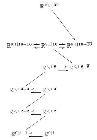
The following is an evident variant of the extensions considered in (CAIB 99, FSS 13).

Proposition

We have

1. The 11d $N = 1$ super-Minkowski spacetime $\mathbb{R}^{10,1\vert \mathbf{32}}$ (def. ) is the central super Lie algebra extension of the 10d type IIA super-Minkowski spacetime $\mathbb{R}^{9,1\vert \mathbf{16}+ \overline{\mathbf{16}}}$ by the 2-cocycle

   $$c_2 \coloneqq \overline{\psi} \wedge \Gamma_{10} \psi \;\;\; \in CE(\mathbb{R}^{9,1\vert \mathbf{16} + \overline{\mathbf{16}}})$$

   (from def. ).

2. The 10d type IIA super-Minkowski spacetime $\mathbb{R}^{9,1\vert \mathbf{16}+ \overline{\mathbf{16}}}$ is central super Lie algebra extension of th 9d $N = 2$ super-Minkowski spacetime by the 2-cocycle given by the type IIA spinor-to-vector pairing

   $$c_2^{IIA} \;\coloneqq\; \overline{\left(\array{\psi_1 \\ \psi_2}\right)} \wedge \Gamma_9^{IIA} \left( \array{\psi_1 \\ \psi_2} \right) \;\;\;\in CE(\mathbb{R}^{8,1\vert \mathbf{16}+ \mathbf{16}})$$

   (from prop. ).

3. The 10d type IIB super-Minkowski spacetime $\mathbb{R}^{9,1\vert \mathbf{16}+ \mathbf{16}}$ is central super Lie algebra extension of th 9d $N = 2$ super-Minkowski spacetime by the 2-cocycle given by the type IIB spinor-to-vector pairing

   $$c_2^{IIB} \;\coloneqq\; \overline{\left(\array{\psi_1 \\ \psi_2}\right)} \wedge \Gamma_9^{IIB} \left( \array{\psi_1 \\ \psi_2} \right) \;\;\; \in CE(\mathbb{R}^{8,1\vert \mathbf{16} + \mathbf{16}})$$

   (from prop. ).

In summary, we have the following diagram in the category of super L-infinity algebras

$$\array{ && && \mathbb{R}^{10,1\vert \mathbf{32}} \\ && && \downarrow \\ \mathbb{R}^{9,1\vert \mathbf{16} + \mathbf{16}} && && \mathbb{R}^{9,1\vert \mathbf{16} + \overline{\mathbf{16}}} &\overset{c_2}{\longrightarrow}& B \mathbb{R} \\ & \searrow && \swarrow \\ && \mathbb{R}^{8,1\vert \mathbf{16} + \mathbf{16}} \\ & {}^{\mathllap{c_2^{IIB}}}\swarrow && \searrow^{\mathrlap{c_2^{IIA}}} \\ B \mathbb{R} && && B \mathbb{R} } \,,$$

where $B\mathbb{R}$ denotes the line Lie 2-algebra, and where each “hook”

$$\array{ \widehat{\mathfrak{g}} \\ \downarrow \\ \mathfrak{g} &\overset{\omega_2}{\longrightarrow}& B\mathbb{R} }$$

is a homotopy fiber sequence (because homotopy fibers of super $L_\infty$-algebra cocycles are the corresponding extension that they classify, see at L-infinity algebra cohomology).

Proof

To see that the given 2-forms are indeed cocycles: they are trivially closed (by def. ), and so all that matters is that we have a well defined super-2-form in the first place. Since the $\psi^\alpha$ are in bidegree $(1,odd)$, they all commutes with each other (see at signs in supergeometry) and hece the condition is that the pairing is symmetric. This is the case by prop. .

Now to see the extensions. Notice that for $\mathfrak{g}$ any (super) Lie algebra (of finite dimension, for convenience), and for $\omega \in \wedge^2\mathfrak{g}^\ast$ a Lie algebra 2-cocycle on it, then the Lie algebra extension $\widehat{\mathfrak{g}}$ that this classifies is neatly characterized in terms of its dual Chevalley-Eilenberg algebra: that is simply the original CE algebra with one new generator $e$ (in degree $(1,even)$) adjoined, and with the differential of $e$ taking to be $\omega$:

$$CE(\widehat{\mathfrak{g}}) = (CE(\mathfrak{g}) \otimes \langle e\rangle), d e = \omega) \,.$$

Hence in the case of $\omega = c_2^{IIA}$ we identify the new generator with $e^9$ and see that the equation $d e^9 = c_2^{IIA}$ is precisely what distinguishes the CE-algebra of $\mathbb{R}^{8,1\vert \mathbf{16}+ \mathbf{16}}$ from that of $\mathbb{R}^{9,1\vert \mathbf{16} + \overline{\mathbf{16}}}$, by prop. and the fact that both spin representation have the same underlying space, by remark .

The other two cases are directly analogous.

Recall the following (e.g. from FSS 16 and references given there):

Definition

The cocycle for the higher WZW term of the Green-Schwarz sigma-model for the M2-brane is

$$\mu_{M2} \coloneqq i\,\overline{\vartheta} \wedge \Gamma_a \Gamma_b \vartheta \wedge e^a \wedge e^b \;\;\; \in CE(\mathbb{R}^{10,1\vert \mathbf{32}})$$

obtained from the spinor-to-bivector pairing of def. . (Here and in the following we are using the nation from remark .)

The cocycle for the WZW term of the Green-Schwarz sigma-model for the type IIA superstring is

$$\mu_{IIA} \coloneqq i\,\overline{\vartheta} \wedge \Gamma_a \Gamma_{10} \vartheta \wedge e^a = i\, \overline{\left( \array{\psi_1 \\ \psi_2} \right)} \Gamma_a \Gamma_{10} \left( \array{\psi_1 \\ \psi_2} \right) \;\;\; \in CE(\mathbb{R}^{9,1\vert \mathbf{16} + \overline{\mathbf{16}}}) \,,$$

i.e. this is the the $e^{10}$-component of $\mu_{M2}$ (“double dimensional reduction” FSS 16):

$$\mu_{IIA} = (\pi_{10})_\ast \mu_{M2} \,.$$

Proposition

The $e^9$-component of the cocycle for the IIA-superstring (def. ), regarded as an element in $CE(\mathbb{R}^{8,1}\vert \mathbf{16} + \mathbf{16})$, equals the 2-cocycle that defines the type IIB extension, according to prop. :

$$(\pi_9)_\ast \mu_{IIA} = c_2^{IIB} \,.$$

Proof

We have

$$\begin{aligned} (\pi_9)_\ast \mu_{IIA} & = i\, \overline{\left( \array{\psi_1 \\ \psi_2} \right)} \Gamma_9 \Gamma_{10} \left( \array{\psi_1 \\ \psi_2} \right) \\ & = \overline{\left(\array{\psi_1 \\ \psi_2}\right)} \Gamma_9^{IIB} \left(\array{\psi_1 \\ \psi_2}\right) \\ & = c_2^{IIB} \end{aligned}$$

where the first equality is by def. , the second is the statement of prop. , while the third is from prop. .

Real spinor representations via Real alternative division algebras

We discuss a close relation between real spin representations and division algebras, due to Kugo-Townsend 82, Sudbery 84 and others: The real spinor representations in dimensions $3,4,6, 10$ happen to have a particularly simple expression in terms of 2-by-2 Hermitian matrices (generalized Pauli matrices) over the four real normed division algebras: the real numbers $\mathbb{R}$ themselves, the complex numbers $\mathbb{C}$, the quaternions $\mathbb{H}$ and the octonions $\mathbb{O}$. Derived from this also the real spinor representations in dimensions $4,5,7,11$ have a fairly simple corresponding expression. We follow the streamlined discussion in Baez-Huerta 09 and Baez-Huerta 10.

Real alternative division algebras

To amplify the following pattern and to fix our notation for algebra generators, recall these definitions:

Definition

(complex numbers)

The complex numbers $\mathbb{C}$ is the commutative algebra over the real numbers $\mathbb{R}$ which is generated from one generators $\{e_1\}$ subject to the relation

• $(e_1)^2 = -1$.

Definition

(quaternions)

The quaternions $\mathbb{H}$ is the associative algebra over the real numbers which is generated from three generators $\{e_1, e_2, e_3\}$ subject to the relations

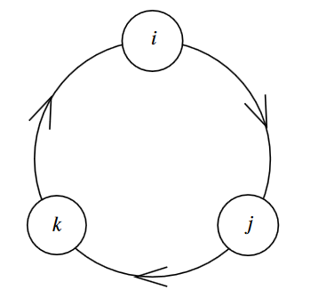
1. for all $i$

   $(e_i)^2 = -1$

2. for $(i,j,k)$ a cyclic permutation of $(1,2,3)$ then

   1. $e_i e_j = e_k$

   2. $e_j e_i = -e_k$

(graphics grabbed from Baez 02)

Definition

(octonions)

The octonions $\mathbb{O}$ is the nonassociative algebra over the real numbers which is generated from seven generators $\{e_1, \cdots, e_7\}$ subject to the relations

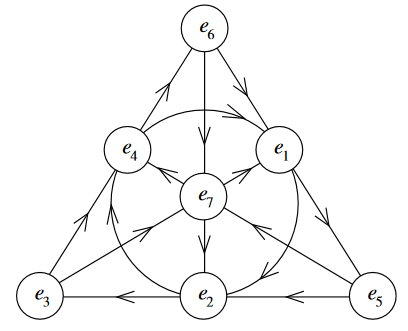
1. for all $i$

   $(e_i)^2 = -1$

2. for $e_i \to e_j \to e_k$ an edge or circle in the diagram shown (a labeled version of the Fano plane) then

   1. $e_i e_j = e_k$

   2. $e_j e_i = -e_k$

   and all relations obtained by cyclic permutation of the indices in these equations.

(graphics grabbed from Baez 02)

One defines the following operations on these real algebras:

Definition

For $\mathbb{K} \in \{\mathbb{R}, \mathbb{C}, \mathbb{H}, \mathbb{O}\}$, let

$$(-)^\ast \;\colon\; \mathbb{K} \longrightarrow \mathbb{K}$$

be the antihomomorphism of real algebras

$$\begin{aligned} (r a)^\ast = r a^\ast &, \text{for}\;\; r \in \mathbb{R}, a \in \mathbb{K} \\ (a b)^\ast = b^\ast a^\ast &,\text{for}\;\; a,b \in \mathbb{K} \end{aligned}$$

given on the generators of def. , def. and def. by

$$(e_i)^\ast = - e_i \,.$$

This operation makes $\mathbb{K}$ into a star algebra. For the complex numbers $\mathbb{C}$ this is called complex conjugation, and in general we call it conjugation.

Let then

$$Re \;\colon\; \mathbb{K} \longrightarrow \mathbb{R}$$

be the function

$$Re(a) \;\coloneqq\; \tfrac{1}{2}(a + a^\ast)$$

(“real part”) and

$$Im \;\colon\; \mathbb{K} \longrightarrow \mathbb{R}$$

be the function

$$Im(a) \;\coloneqq \; \tfrac{1}{2}(a - a^\ast)$$

(“imaginary part”).

It follows that for all $a \in \mathbb{K}$ then the product of a with its conjugate is in the real center of $\mathbb{K}$

$$a a^\ast = a^\ast a \;\in \mathbb{R} \hookrightarrow \mathbb{K}$$

and we write the square root of this expression as

$${\vert a\vert} \;\coloneqq\; \sqrt{a a^\ast}$$

called the norm or absolute value function

$${\vert -\vert} \;\colon\; \mathbb{K} \longrightarrow \mathbb{R} \,.$$

This norm operation clearly satisfies the following properties (for all $a,b \in \mathbb{K}$)

1. $\vert a \vert \geq 0$;

2. ${\vert a \vert } = 0 \;\;\;\;\; \Leftrightarrow\;\;\;\;\;\; a = 0$;

3. ${\vert a b \vert } = {\vert a \vert} {\vert b \vert}$

and hence makes $\mathbb{K}$ a normed algebra.

Since $\mathbb{R}$ is a division algebra, these relations immediately imply that each $\mathbb{K}$ is a division algebra, in that

$$a b = 0 \;\;\;\;\;\; \Rightarrow \;\;\;\;\;\; a = 0 \;\; \text{or} \;\; b = 0 \,.$$

Hence the conjugation operation makes $\mathbb{K}$ a real normed division algebra.

Remark

Sending each generator in def. , def. and def. to the generator of the same name in the next larger algebra constitutes a sequence of real star-algebra homomorphisms

$$\mathbb{R} \hookrightarrow \mathbb{C} \hookrightarrow \mathbb{H} \hookrightarrow \mathbb{O} \,.$$

Proposition

(Hurwitz theorem: $\mathbb{R}$, $\mathbb{C}$, $\mathbb{H}$ and $\mathbb{O}$ are the normed real division algebras)

The four algebras of real numbers $\mathbb{R}$, complex numbers $\mathbb{C}$, quaternions $\mathbb{H}$ and octonions $\mathbb{O}$ from def. , def. and def. respectively, which are real normed division algebras via def. , are, up to isomorphism, the only real normed division algebras that exist.

Remark

While hence the sequence from remark

$$\mathbb{R} \hookrightarrow \mathbb{C} \hookrightarrow \mathbb{H} \hookrightarrow \mathbb{O}$$

is maximal in the category of real normed non-associative division algebras, there is a pattern that does continue if one disregards the division algebra property. Namely each step in this sequence is given by a construction called forming the Cayley-Dickson double algebra. This continues to an unbounded sequence of real nonassociative star-algebras

$$\mathbb{R} \hookrightarrow \mathbb{C} \hookrightarrow \mathbb{H} \hookrightarrow \mathbb{O} \hookrightarrow \mathbb{S} \hookrightarrow \cdots$$

where the next algebra $\mathbb{S}$ is called the sedenions.

What actually matters for the following relation of the real normed division algebras to real spin representations is that they are also alternative algebras:

Definition

(alternative algebra)

Given any non-associative algebra $A$, then the trilinear map

$$[-,-,-] \;-\; A \otimes A \otimes A \longrightarrow A$$

given on any elements $a,b,c \in A$ by

$$[a,b,c] \coloneqq (a b) c - a (b c)$$

is called the associator (in analogy with the commutator $[a,b] \coloneqq a b - b a$ ).

If the associator is completely antisymmetric (in that for any permutation $\sigma$ of three elements then $[a_{\sigma_1}, a_{\sigma_2}, a_{\sigma_3}] = (-1)^{\vert \sigma\vert} [a_1, a_2, a_3]$ for $\vert \sigma \vert$ the signature of the permutation) then $A$ is called an alternative algebra.

If the characteristic of the ground field is different from 2, then alternativity is readily seen to be equivalent to the conditions that for all $a,b \in A$ then

$$(a a)b = a (a b) \;\;\;\;\; \text{and} \;\;\;\;\; (a b) b = a (b b) \,.$$

We record some basic properties of associators in alternative star-algebras that we need below:

Proposition

(properties of alternative star algebras)

Let $A$ be an alternative algebra (def. ) which is also a star algebra. Then

1. the associator vanishes when at least one argument is real

   $$[Re(a),b,c]$$

2. the associator changes sign when one of its arguments is conjugated

   $$[a,b,c] = -[a^\ast,b,c] \,;$$

3. the associator vanishes when one of its arguments is the conjugate of another:

   $$[a,a^\ast, b] = 0 \,;$$

4. the associator is purely imaginary

   $$Re([a,b,c]) = 0 \,.$$

Proof

That the associator vanishes as soon as one argument is real is just the linearity of an algebra product over the ground ring.

Hence in fact

$$[a,b,c] = [Im(a), Im(b), Im(c)] \,.$$

This implies the second statement by linearity. And so follows the third statement by skew-symmetry:

$$[a,a^\ast,b] = -[a,a,b] = 0 \,.$$

The fourth statement finally follows by this computation:

$$\begin{aligned} [a,b,c]^\ast & = -[c^\ast, b^\ast, a^\ast] \\ & = -[c,b,a] \\ & = -[a,b,c] \end{aligned} \,.$$

Here the first equation follows by inspection and using that $(a b)^\ast = b^\ast a^\ast$, the second follows from the first statement above, and the third is the ant-symmetry of the associator.

It is immediate to check that:

Proposition

($\mathbb{R}$, $\mathbb{C}$, $\mathbb{H}$ and $\mathbb{O}$ are real alternative algebras)

The real algebras of real numbers, complex numbers, def. ,quaternions def. and octonions def. are alternative algebras (def. ).

Proof

Since the real numbers, complex numbers and quaternions are associative algebras, their associator vanishes identically. It only remains to see that the associator of the octonions is skew-symmetric. By linearity it is sufficient to check this on generators. So let $e_i \to e_j \to e_k$ be a circle or a cyclic permutation of an edge in the Fano plane. Then by definition of the octonion multiplication we have

$$\begin{aligned} (e_i e_j) e_j &= e_k e_j \\ &= - e_j e_k \\ & = -e_i \\ & = e_i (e_j e_j) \end{aligned}$$

and similarly

$$\begin{aligned} (e_i e_i ) e_j &= - e_j \\ &= - e_k e_i \\ &= e_i e_k \\ &= e_i (e_i e_j) \end{aligned} \,.$$

The analog of the Hurwitz theorem (prop. ) is now this:

Proposition

($\mathbb{R}$, $\mathbb{C}$, $\mathbb{H}$ and $\mathbb{O}$ are precisely the alternative real division algebras)

The only division algebras over the real numbers which are also alternative algebras (def. ) are the real numbers themselves, the complex numbers, the quaternions and the octonions from prop. .

This is due to (Zorn 30).

For the following, the key point of alternative algebras is this equivalent characterization:

Proposition

(alternative algebra detected on subalgebras spanned by any two elements)

A nonassociative algebra is alternative, def. , precisely if the subalgebra? generated by any two elements is an associative algebra.

This is due to Emil Artin, see for instance (Schafer 95, p. 18).

Proposition is what allows to carry over a minimum of linear algebra also to the octonions such as to yield a representation of the Clifford algebra on $\mathbb{R}^{9,1}$. This happens in the proof of prop. below.

So we will be looking at a fragment of linear algebra over these four normed division algebras. To that end, fix the following notation and terminology:

Definition

(hermitian matrices with vaues in real normed division algebras)

Let $\mathbb{K}$ be one of the four real normed division algebras from prop. , hence equivalently one of the four real alternative division algebras from prop. .

Say that an $n \times n$ matrix with coefficients in $\mathbb{K}$, $A\in Mat_{n\times n}(\mathbb{K})$ is a hermitian matrix if the transpose matrix $(A^t)_{i j} \coloneqq A_{j i}$ equals the componentwise conjugated matrix (def. ):

$$A^t = A^\ast \,.$$

Hence with the notation

$$(-)^\dagger \coloneqq ((-)^t)^\ast$$

then $A$ is a hermitian matrix precisely if

$$A = A^\dagger \,.$$

We write $Mat_{2 \times 2}^{her}(\mathbb{K})$ for the real vector space of hermitian matrices.

Definition

(trace reversal)

Let $A \in Mat_{2 \times 2}^{her}(\mathbb{K})$ be a hermitian $2 \times 2$ matrix as in def. . Its trace reversal is the result of subtracting its trace times the identity matrix:

$$\tilde A \;\coloneqq\; A - (tr A) 1_{n\times n} \,.$$

Spacetime in dimensions 3,4,6 and 10

We discuss how Minkowski spacetime of dimension 3,4,6 and 10 is naturally expressed in terms of the real normed division algebras $\mathbb{K}$ from prop. , equivalently the real alternative division algebras from prop. .

Proposition

(Minkowski spacetime via hermitian matrices in real normed division algebras)

Let $\mathbb{K}$ be one of the four real normed division algebras from prop. , hence one of the four real alternative division algebras from prop. .

There is a isomorphism (of real inner product spaces) between Minkowski spacetime (def. ) of dimension

$$d = 2 + dim_{\mathbb{R}}(\mathbb{K})$$

hence

1. $\mathbb{R}^{2,1}$ for $\mathbb{K} = \mathbb{R}$;

2. $\mathbb{R}^{3,1}$ for $\mathbb{K} = \mathbb{C}$;

3. $\mathbb{R}^{5,1}$ for $\mathbb{K} = \mathbb{H}$;

4. $\mathbb{R}^{9,1}$ for $\mathbb{K} = \mathbb{O}$.

and the real vector space of $2 \times 2$ hermitian matrices over $\mathbb{K}$ (def. ) equipped with the inner product whose norm-square is the negative of the determinant operation on matrices:

$$\mathbb{R}^{dim_{\mathbb{R}}(\mathbb{K})+1,1} \;\simeq\; \left(Mat_{2 \times 2}^{her}(\mathbb{K}), -det \right) \,.$$

As a linear map this is given by

$$(x_0, x_1, \cdots, x_{d-1}) \;\mapsto\; \left( \array{ x_0 + x_1 & y \\ y^\ast & x_0 - x_1 } \right) \;\;\; \text{with}\; y \coloneqq x_2 1 + x_3 e_1 + x_4 e_2 + \cdots + x_{2 + dim_{\mathbb{R}(\mathbb{K})}} \,e_{dim_{\mathbb{R}}(\mathbb{K})-1} \,.$$

Under this identification the operation of trace reversal from def. corresponds to time reversal in that

$$\widetilde{ \left( \array{ x_0 + x_1 & y \\ y^\ast & x_0 - x_1 } \right) } \;=\; \left( \array{ -x_0 + x_1 & y \\ y^\ast & -x_0 - x_1 } \right) \,.$$

Proof

This is immediate from the nature of the conjugation operation $(-)^\ast$ from def. :

$$\begin{aligned} - det \left( \array{ x_0 + x_1 & y \\ y^\ast & x_0 - x_1 } \right) & = -(x_0 + x_1)(x_0 - x_1) + y y^\ast \\ & = -(x_0)^2 + \underoverset{a = 1}{d-1}{\sum} (x_a)^2 \end{aligned} \,.$$

By direct computation one finds:

Proposition

In terms of the trace reversal operation $\widetilde{(-)}$ from def. , the determinant operation on hermitian matrices (def. ) has the following alternative expression

$$\begin{aligned} -det(A) & = A \tilde A \\ & = \tilde A A \end{aligned} \,.$$

and the Minkowski inner product has the alternative expression

$$\eta(A,B) = \tfrac{1}{2}Re(tr(A \tilde B)) = \tfrac{1}{2} Re(tr(\tilde A B)) \,.$$

(Baez-Huerta 09, prop. 5)

Real spinors in dimensions 3, 4, 6 and 10

We now discuss how real spin representations in dimensions 3,4, 6 and 10 are naturally induced from linear algebra over the four real alternative division algebras.

In particular we establish the following table of exceptional isomorphisms of spin groups:

exceptional spinors and real normed division algebras

Lorentzian spacetime dimension	$\phantom{AA}$spin group	normed division algebra	$\,\,$ brane scan entry
$3 = 2+1$	$Spin(2,1) \simeq SL(2,\mathbb{R})$	$\phantom{A}$ $\mathbb{R}$ the real numbers	super 1-brane in 3d
$4 = 3+1$	$Spin(3,1) \simeq SL(2, \mathbb{C})$	$\phantom{A}$ $\mathbb{C}$ the complex numbers	super 2-brane in 4d
$6 = 5+1$	$Spin(5,1) \simeq$ SL(2,H)	$\phantom{A}$ $\mathbb{H}$ the quaternions	little string
$10 = 9+1$	Spin(9,1) ${\simeq}$ “SL(2,O)”	$\phantom{A}$ $\mathbb{O}$ the octonions	heterotic/type II string

Remark

Prop. immediately implies that for $\mathbb{K} \in \{\mathbb{R}, \mathbb{C}, \mathbb{H}\}$ then there is a monomorphism from the special linear group $SL(2,\mathbb{K})$ (see at SL(2,H) for the definition in the quaternionic case) to the spin group in the given dimension:

$$SL(2,\mathbb{K}) \hookrightarrow Spin(dim_{\mathbb{R}(\mathbb{K} )} +1 ,1)$$

given by

$$A \mapsto A(-)A^\dagger \,.$$

This preserves the determinant, and hence the Lorentz form, by the multiplicative property of the determinant:

$$det(A(-)A^\dagger) = \underset{=1}{\underbrace{det(A)}} det(-) \underset{= 1}{\underbrace{det(A)}}^\ast = det(-) \,.$$

Hence it remains to show that this is surjective, and to define this action also for $\mathbb{K}$ being the octonions, where general matrix calculus does not apply, due to non-associativity.

Definition

(Clifford algebra via normed division algebra)

Let $\mathbb{K}$ be one of the four real normed division algebras from prop. , hence one of the four real alternative division algebras from prop. .

Define a real linear map

$$\Gamma \;\colon\; \mathbb{R}^{dim_{\mathbb{R}}(\mathbb{K})+1,1} \simeq End_{\mathbb{R}}(\mathbb{K}^4)$$

from (the real vector space underlying) Minkowski spacetime to real linear maps on $\mathbb{K}^4$

$$\Gamma(A) \left( \array{ \psi \\ \phi } \right) \;\coloneqq\; \left( \array{ \tilde A \phi \\ A \psi } \right) \,.$$

Here on the right we are using the isomorphism from prop. for identifying a spacetime vector with a $2 \times 2$-matrix, and we are using the trace reversal $\widetilde(-)$ from def. .

Remark

Each operation of $\Gamma(A)$ in def. is clearly a linear map, even for $\mathbb{K}$ being the non-associative octonions. The only point to beware of is that for $\mathbb{K}$ the octonions, then the composition of two such linear maps is not in general given by the usual matrix product.

Proposition

(real spin representations via normed division algebras)

The map $\Gamma$ in def. gives a representation of the Clifford algebra $Cl(\mathbb{R}^{dim_{\mathbb{R}}}(\mathbb{K}+1,1) )$ (def. ), i.e of

1. $Cl(\mathbb{R}^{2,1})$ for $\mathbb{K} = \mathbb{R}$;

2. $Cl(\mathbb{R}^{3,1})$ for $\mathbb{K} = \mathbb{C}$;

3. $Cl(\mathbb{R}^{5,1})$ for $\mathbb{K} = \mathbb{H}$;

4. $Cl(\mathbb{R}^{9,1})$ for $\mathbb{K} = \mathbb{O}$.

Hence this Clifford representation induces representations of the spin group $Spin(dim_{\mathbb{R}}(\mathbb{K})+1,1)$ on the real vector spaces

$$S_{\pm } \coloneqq \mathbb{K}^2 \,.$$

(Baez-Huerta 09, p. 6)

Proof

We need to check that the Clifford relation

$$(\Gamma(A))^2 = -\eta(A,A)1$$

is satisfied. Now by definition, for any $(\phi,\psi) \in \mathbb{K}^4$ then

$$(\Gamma(A))^2 \left( \array{ \phi \\ \psi } \right) \;=\; \left( \array{ \tilde A(A \phi) \\ A(\tilde A \psi) } \right) \,,$$

where on the right we have in each component ordinary matrix product expressions.

Now observe that both expressions on the right are sums of triple products that involve either one real factor or two factors that are conjugate to each other:

$$\begin{aligned} A (\tilde A \psi) & = \left( \array{ x_0 + x_1 & y \\ y^\ast & x_0 - x_1 } \right) \cdot \left( \array{ (-x_0 + x_1) \phi_1 + y \phi_2 \\ y^\ast \phi_1 - (x_0 + x_1)\phi_2 } \right) \\ & = \left( \array{ (-x_0^2 + x_1^2) \phi_1 + (x_0 + x_1)(y \phi_2) + y (y^\ast \phi_1) - y( (x_0 + x_1) \phi_2 ) \\ \cdots } \right) \end{aligned} \,.$$

Since the associators of triple products that involve a real factor and those involving both an element and its conjugate vanish by prop. (hence ultimately by Artin’s theorem, prop. ). In conclusion all associators involved vanish, so that we may rebracket to obtain

$$(\Gamma(A))^2 \left( \array{ \phi \\ \psi } \right) \;=\; \left( \array{ (\tilde A A) \phi \\ (A \tilde A) \psi } \right) \,.$$

This implies the statement via the equality $A \tilde A = \tilde A A = -det(A)$ (prop. ).

Remark

(index notation for generalized Pauli matrices)

Prop. says that the isomorphism of prop. is that given by forming generalized Pauli matrices. In standard physics notation these matrices are written as

$$\Gamma(x^a) = (\gamma^a_{\alpha \dot \alpha}) \,.$$

Proposition

The spin representations given via prop. by the Clifford representation of def. are the following:

1. for $\mathbb{K} = \mathbb{R}$ the Majorana representation of $Spin(2,1)$ on $S_+ \simeq S_-$;

2. for $\mathbb{K} = \mathbb{C}$ the Majorana representation of $Spin(3,1)$ on $S_+ \simeq S_-$;

3. for $\mathbb{K} = \mathbb{H}$ the Weyl representation of $Spin(5,1)$ on $S_+$ and on $S_-$;

4. for $\mathbb{K} = \mathbb{O}$ the Majorana-Weyl representation of $Spin(9,1)$ on $S_+$ and on $S_-$.

Proposition

(spinor bilinear pairings)

Under the identification of prop. the bilinear pairings

$$\overline{(-)}(-) \;\colon\; S_+ \otimes S_-\longrightarrow \mathbb{R}$$

and

$$\overline{(-)}\Gamma (-) \;\colon\; S_\pm \otimes S_{\pm}\longrightarrow V$$

from above are given, respectively, by forming the real part of the canonical $\mathbb{K}$-inner product

$$\overline{(-)}(-) \colon S_+\otimes S_- \longrightarrow \mathbb{R}$$

$$(\psi,\phi)\mapsto \overline{\psi} \phi \coloneqq Re(\psi^\dagger \cdot \phi)$$

and by forming the product of a column vector with a row vector to produce a matrix, possibly up to trace reversal (def. ):

$$S_+ \otimes S_+ \longrightarrow V$$

$$(\psi , \phi) \mapsto \overline{\psi}\Gamma \phi \coloneqq \widetilde{\psi \phi^\dagger + \phi \psi^\dagger}$$

and

$$S_- \otimes S_- \longrightarrow V$$

$$(\psi , \phi) \mapsto {\psi \phi^\dagger + \phi \psi^\dagger}$$

For $A \in V$ the $A$-component of this map is

$$\eta(\overline{\psi}\Gamma \phi, A) = Re (\psi^\dagger (A\phi)) \,.$$

(Baez-Huerta 09, prop. 8, prop. 9).

Example

(real spin representation in $d = 2+1$)

Consider the case $\mathbb{K} = \mathbb{R}$ of real numbers.

Now $V= Mat^{symm}_{2\times 2}(\mathbb{R})$ is the space of symmetric 2x2-matrices with real numbers.

$$V = \left\{ \left. \left( \array{ t + x & y \\ y & t - x } \right) \right\vert t,x,y\in \mathbb{R} \right\}$$

The “light-cone”-basis for this space would be

$$\left\{ v^+ \coloneqq \left( \array{ 1 & 0 \\ 0 & 0 } \right) \,, \; v^- \coloneqq \left( \array{ 0 & 0 \\ 0 & 1 } \right) \,, \; v^y \coloneqq \left( \array{ 0 & 1 \\ 1 & 0 } \right) \right\}$$

Its trace reversal (def. ) is

$$\left\{ \tilde{v}^+ \coloneqq \left( \array{ 0 & 0 \\ 0 & -1 } \right) \,, \; \tilde v^- \coloneqq \left( \array{ -1 & 0 \\ 0 & 0 } \right) \,, \; \tilde v^y \coloneqq \left( \array{ 0 & 1 \\ 1 & 0 } \right) \right\}$$

Hence the Minkowski metric of prop. in this basis has the components

$$\eta = \left( \array{ 0 & -1 & 0 \\ -1 & 0 & 0 \\ 0 & 0 & 2 } \right) \,.$$

As vector spaces $S_{\pm} = \mathbb{R}^2$.

The bilinear spinor pairing $\overline{(-)}(-) \colon S_+ \otimes S_- \to \mathbb{R}$ is given by

$$\begin{aligned} \overline{\psi}\phi &= \psi^t \cdot \phi \\ & = \psi_1 \phi_1 + \psi_2 \phi_2 \end{aligned} \,.$$

The spinor pairing $S_+ \otimes S_+ \otimes V^\ast \to \mathbb{R}$ from prop. is given on an $A = A_+ v^+ + A_- v^- + A_y v^y$ ($A_+, A_-, A_y \in \mathbb{R}$) by the components

$$\begin{aligned} \eta(\overline{\psi}\Gamma\phi,A) &= \psi^t \cdot A \cdot \phi \\ & = \psi_1 \phi_1 A_+ + \psi_2 \phi_2 A_- + (\psi_1 \phi_2 + \psi_2 \phi_1) A_y \end{aligned}$$

and $S_- \otimes S_- \otimes V^\ast \to \mathbb{R}$ is given by the components

$$\begin{aligned} \eta(\overline{\psi}\Gamma\phi,A) &= \psi^t \cdot \tilde A \cdot \phi \\ &= -\psi_1 \phi_1 A_+ - \psi_2 \phi_2 A_- + (\psi_1 \phi_2 + \psi_2 \phi_1) A_y \end{aligned} \,.$$

and so, in view of the above metric components, in terms of dual bases $\{\psi^i\}$ this is

$$\mu = - \psi^1 \otimes \psi^1 \otimes A_- - \psi^2 \otimes \psi^2 \otimes A_+ + \frac{1}{2} (\psi^1 \otimes \psi^2 \oplus \psi^2 \otimes\psi^1) \otimes A_y$$

So there is in particular the 2-dimensional space of isomorphisms of super Minkowski spacetime super translation Lie algebras

$$\mathbb{R}^{2,1|\mathbf{2}} \stackrel{\simeq}{\longrightarrow} \mathbb{R}^{2,1|\bar\mathbf{2}}$$

(not though of the corresponding super Poincaré Lie algebras, because for them the difference in the Spin-representation does matter) spanned by

$$(\theta_1,\theta_2, \vec e) \mapsto (\theta_1, -\theta_2, -\vec e)$$

and by

$$(\theta_1,\theta_2, \vec e) \mapsto (-\theta_1, \theta_2, -\vec e) \,.$$

Hence there is a 1-dimensional space of non-trivial automorphism

$$\mathbb{R}^{2,1|\mathbf{2}} \stackrel{\simeq}{\longrightarrow} \mathbb{R}^{2,1|\mathbf{2}}$$

spanned by

$$(\theta_1,\theta_2, \vec e) \mapsto (-\theta_1, -\theta_2, \vec e) \,.$$

Real spinors in dimensions 4,5,7 and 11

Definition

Write $V \coloneqq Mat^{hermitian}_{2\times 2}(\mathbb{K}) \oplus \mathbb{R}$.

Write $S \coloneqq \mathbb{K}^4$. Define a real linear map

$$\Gamma \;\colon\; V\longrightarrow End(S)$$

given by left matrix multiplication

$$\Gamma(A,a) \coloneqq \left( \array{ a \cdot 1_{2\times 2} & \tilde A \\ A & -a \cdot 1_{2\times 2} } \right) \,.$$

Remark

The real vector space $V$ in def. equipped with the inner product $\eta(-,-)$ given by

$$\eta((A,a), (A,a)) = det(A) + a^2$$

is Minkowski spacetime

1. $\mathbb{R}^{3,1}$ for $\mathbb{K} = \mathbb{R}$;

2. $\mathbb{R}^{4,1}$ for $\mathbb{K} = \mathbb{C}$;

3. $\mathbb{R}^{6,1}$ for $\mathbb{K} = \mathbb{H}$;

4. $\mathbb{R}^{10,1}$ for $\mathbb{K} = \mathbb{O}$.

Proposition

The map $\Gamma$ in def. gives a representation of the Clifford algebra of

1. $\mathbb{R}^{3,1}$ for $\mathbb{K} = \mathbb{R}$;

2. $\mathbb{R}^{4,1}$ for $\mathbb{K} = \mathbb{C}$;

3. $\mathbb{R}^{6,1}$ for $\mathbb{K} = \mathbb{H}$;

4. $\mathbb{R}^{10,1}$ for $\mathbb{K} = \mathbb{O}$.

Under restriction along $Spin(n+2,1) \hookrightarrow Cl(n+2,1)$ this is isomorphic to

1. for $\mathbb{K} = \mathbb{R}$ the Majorana representation of $Spin(3,1)$ on $S$;

2. for $\mathbb{K} = \mathbb{C}$ the Dirac representation of $Spin(4,1)$ on $S$;

3. for $\mathbb{K} = \mathbb{H}$ the Dirac representation of $Spin(6,1)$ on $S$;

4. for $\mathbb{K} = \mathbb{O}$ the Majorana representation of $Spin(10,1)$ on $S$.

(Baez-Huerta 10, p. 10, prop. 8, prop. 9)

Write

$$\Gamma^0 \coloneqq \left( \array{ 0 & - 1_{2x2} \\ 1_{2\times 2} & 0 } \right) \,.$$

Proposition

Under the identification of prop. of the bilinear pairings

$$\overline{(-)}(-) \;\colon\; S \otimes S \longrightarrow \mathbb{R}$$

and

$$\overline{(-)}\Gamma (-) \;\colon\; S \otimes S \longrightarrow V$$

of remark , the first is given by

$$(\psi,\phi) \mapsto \overline\psi\phi \coloneqq Re(\psi^\dagger \Gamma^0 \phi)$$

and the second is characterized by

$$\begin{aligned} \eta \left( \overline{\psi}\Gamma\phi, A \right) &= \overline{\psi}(\Gamma(A)\phi) \\ & = Re( \psi^\dagger \Gamma^0 \Gamma(A)\phi) \end{aligned} \,.$$

(Baez-Huerta 10, prop. 10, prop. 11).

Real pinor representations (including spacetime reflection)

We discuss Pin(10,1)-representations when using the spinor conventions from CDF, II.7.1, as in Prop. above.

The statement is Prop. below. We need the following facts from the above discussion:

Dirac representation. From Prop. 2.18 we have

(1)$$\Gamma_0^\dagger = + \Gamma_0 \phantom{AAAA} \Gamma_{a}^\dagger = - \Gamma_{a} \phantom{AAA} \text{for} \; a \; \text{spatial}$$

Charge conjugation matrix. From Prop. 2.22 and Remark 2.23 we get for $d = 11$ (see the table there) that the charge conjugation matrix satisfies

(2)$$\Gamma_a^T C = - C \Gamma_a$$

Majorana condition. From Prop. 2.29 we have that the Majorana condition on $\psi$ is equivalent to

(3)$$\psi^\dagger \Gamma_0 = \psi^t C$$

Proposition

(Pin group-representation on Majorana spinors)

For $p+1 = 10+1$ and with choice of Dirac representation from Prop. , multiplication by $\Gamma_{a}$ does not preserves the Majorana spinor condition (3). But multiplication by $\pm i \Gamma_{a}$ does.

Hence to get on Majorana spinors not just a Spin group-representation, but even a Pin group-representation (incluing spacetime reflections on top of rotations) in the spinor convention of Prop. , one needs to use the Cliffor algebra generated from $\{i \Gamma_a\}_{a - 0}^p$

Proof

First assume that the index is spatial. Suppose $\psi$ is Majorana, then we compute as follows:

$$\begin{aligned} (\Gamma_a \psi)^T C & = \psi^T \Gamma_a^T C \\ & = - \psi^T C \Gamma_a \\ & = - \psi^\dagger \Gamma_0 \Gamma_a \\ & = + \psi^\dagger \Gamma_a \Gamma_0 \\ & = - \psi^\dagger \Gamma_a^\dagger \Gamma_0 \\ & = - (\Gamma_a \psi)^\dagger \Gamma_0 \end{aligned}$$

Here

• the first equality is that transposition is an algbra anti-homomorphism,

• the second equality is the charge conjugation relation (2),

• the third equality is the Majorana condition (3) on $\psi$,

• the fourth equality is the Clifford relation $\{\Gamma_0,\Gamma_{a}\} = 0$,

• the fifth equality is the anti-hermiticity (1),

• the sixth equality is that $\dagger$ is algebra anti-homomorphism.

In conclusion, the overall minus sign between the first and the last term means that $\Gamma_{a} \psi$ fails the Majorana condition (3).

But with $i \Gamma_{a}$ instead of $\Gamma_{a}$, the same computation applies, except that there is one extra sign when $\dagger$ is applied, from $i^\dagger = i^\ast = -i$. Hence this fixes the sign.

Finally, in the case that $a = 0$ the same computation goes through once more, except for two extra signs: One from the difference of sign under $\dagger$ from (1), the other due to the difference of sign in commuting through $\Gamma_0$. Hence the conclusion remains the same.

Spacetime supersymmetry

We have seen in example that super-extensions of the symmetries of Minkowski spacetime are given by real spin representations, and then we constructed and classified these (above).

Hence every real spin representation of $Spin(d-1,1)$ induces a super Lie algebra extension of the Poincaré Lie algebra $\mathfrak{Iso}(\mathbb{R}^{d-1,1})$ in that dimension, i.e. of the Lie algebra of the isometry group of the Minkowski spacetime (def. ) in that dimension. These are the supersymmetry algebras in physics.

Since we may recover a Minkowski spacetime from its Poincaré Lie algebra as the (vector space underlying the) coset of the Poincaré Lie algebra by the Lie algebra $\mathfrak{so}(d-1,1)$ of the spin group (the orthogonal Lie algebra in Lorentzian signature)

$$\mathbb{R}^{d-1,1} \simeq \mathfrak{Iso}(\mathbb{R}^{d-1,1})/\mathfrak{so}(d-1,1)$$

(namely as the Lie algebra of translations along itself), every super Lie algebra extension of the Poincaré Lie algebra defines a super Lie algebra extension of Minkowski spacetime. These extensions are the super Minkowski spacetimes $\mathbb{R}^{d-1,1\vert N}$ which in the physics literature are often just called “superspace”.

To set the scene, we recall some basics of ordinary spacetime symmetry in

• Spacetime symmetry

Then in

• Super Poincaré and super Minkowski symmetry

we specialize to the particular such extensions commonly known as supersymmetries.

Finally we discuss the question of how god-given this common choice is, in

• Supersymmetry from the superpoint

Spacetime symmetry

Definition

For $d \in \mathbb{N}$, write $\mathbb{R}^{d-1,1}$ for Minkowski spacetime (def. ), regarded as the inner product space whose underlying vector space is $\mathbb{R}^d$ and equipped with the bilinear form given in the canonical linear basis of $\mathbb{R}^d$ by

$$\eta \coloneqq diag(-1,+1,+1, \cdots, +1) \,.$$

The Poincaré group $Iso(\mathbb{R}^{d-1,1})$ is the isometry group of this inner product space. The Poincaré Lie algebra $\mathfrak{iso}(\mathbb{R}^{d-1,1})$ is the Lie algebra of this Lie group (its Lie differentiation)

$$\mathfrak{iso}(\mathbb{R}^{d-1,1}) \coloneqq Lie(Iso(\mathbb{R}^{d-1,1})) \,.$$

Remark

The Poincaré group is the semidirect product group

$$Iso(\mathbb{R}^{d-1,1}) \simeq \mathbb{R}^{d-1,1} \rtimes O(d-1,1)$$

of the Lorentz group $O(d-1,1)$ (the group of linear isometries of Minkowski spacetime) with the $\mathbb{R}^d$ regarded as the translation group along itself, via the defining action.

Accordingly, the Poincaré Lie algebra is the semidirect product Lie algebra

$$\mathfrak{iso}(\mathbb{R}^{d-1,1}) \simeq \mathbb{R}^{d-1,1} \rtimes \mathfrak{so}^+(d-1,1)$$

of the abelian Lie algebra on $\mathbb{R}^d$ with the (orthochronous) special orthogonal Lie algebra $\mathfrak{so}(d-1,1)$.

Proposition

For $\{P_a\}$ the canonical linear basis of $\mathbb{R}^d$, and for $\{L_{a b} = - L_{b a}\}$ the corresponding canonical basis of $\mathfrak{so}(d-1,1)$, then the Lie bracket in $\mathfrak{iso}(\mathbb{R}^{d-1,1})$ is given as follows:

$$\begin{aligned} [P_a, P_b] & = 0 \\ [L_{a b}, L_{c d}] & = \eta_{d a} L_{b c} -\eta_{b c} L_{a d} +\eta_{a c} L_{b d} -\eta_{d b} L_{a c} \\ [L_{a b}, P_c] & = \eta_{a c} P_b -\eta_{bc} P_a \end{aligned}$$

Proof

Since Lie differentiation sees only the connected component of a Lie group, and does not distinguish betwee a Lie group and any of its discrete covering spaces, we may equivalently consider the Lie algebra of the spin group $Spin(d-1,1) \to SO^+(d-1,1)$ (the double cover of the proper orthochronous Lorentz group) and its action on $\mathbb{R}^{d-1,1}$.

By the discussion at spin group, the Lie algebra of $Spin(d-1,1)$ is the Lie algebra spanned by the Clifford algebra bivectors

$$L_{a b} \leftrightarrow \Gamma_a \Gamma_b$$

and its action on itself as well as on the vectors, identified with single Clifford generators

$$P_a \leftrightarrow \Gamma_a$$

is given by forming commutators in the Clifford algebra:

$$[L_{a b}, P_c] \leftrightarrow \tfrac{1}{2}[\Gamma_{a b}, \Gamma_c ]$$

$$[L_{a b}, L_{c d}] \leftrightarrow \tfrac{1}{2}[\Gamma_{a b}, \Gamma_{c d} ] \,.$$

Via the Clifford relation

$$\Gamma_a \Gamma_b + \Gamma_b \Gamma_a = -2 \eta_{a b}$$

this yields the claim.

Remark

Dually, the Chevalley-Eilenberg algebra $CE(\mathfrak{iso}(\mathbb{R}^{d-1})$ is generated from $\mathbb{R}^{d,1}$ and $\wedge^2 \mathbb{R}^{d,1}$. For $\{t_a\}$ the standard basis of $\mathbb{R}^{d-1,1}$ we write $\{\omega^{a b}\}$ and $\{e^a\}$ for these generators. With $(\eta_{a b})$ the components of the Minkowski metric we write

$$\omega^{a}{}_b \coloneqq \omega^{a c}\eta_{c b} \,.$$

In terms of this the CE-differential that defines the Lie algebra structure is

$$d_{CE} \colon \omega^{a b} = \omega^a{}_c \wedge \omega^{c b}$$

$$d_{CE} \colon e^a \mapsto \omega^{a}{}_b \wedge t^b$$

Super Poincaré and super Minkowski symmetry

We may now finally make explicit the super-extension of spacetime symmetry according to example :

In all of the following it is most convenient to regard super Lie algebras dually via their Chevalley-Eilenberg algebras:

Definition

For $\mathfrak{g}$ a super Lie algebra of finite dimension, then its Chevalley-Eilenberg algebra $CE(\mathfrak{g})$ is the super-Grassmann algebra on the dual super vector space

$$\wedge^\bullet \mathfrak{g}^\ast$$

equipped with a differential $d_{\mathfrak{g}}$ that on generators is the linear dual of the super Lie bracket

$$d_{\mathfrak{g}} \;\coloneqq\; [-,-]^\ast \;\colon\; \mathfrak{g}^\ast \to \mathfrak{g}^\ast \wedge \mathfrak{g}^\ast$$

and which is extended to $\wedge^\bullet \mathfrak{g}^\ast$ by the graded Leibniz rule (i.e. as a graded derivation).

$\,$

Here all elements are $(\mathbb{Z} \times \mathbb{Z}/2)$-bigraded, the first being the cohomological grading $n$ in $\wedge^\n \mathfrak{g}^\ast$, the second being the super-grading $\sigma$ (even/odd).

For $\alpha_i \in CE(\mathfrak{g})$ two elements of homogeneous bi-degree $(n_i, \sigma_i)$, respectively, the sign rule is

$$\alpha_1 \wedge \alpha_2 = (-1)^{n_1 n_2} (-1)^{\sigma_1 \sigma_2}\; \alpha_2 \wedge \alpha_1 \,.$$

(See at signs in supergeometry for discussion of this sign rule and of an alternative sign rule that is also in use. )

We may think of $CE(\mathfrak{g})$ equivalently as the dg-algebra of left-invariant super differential forms on the corresponding simply connected super Lie group .

The concept of Chevalley-Eilenberg algebras is traditionally introduced as a means to define Lie algebra cohomology:

Definition

Given a super Lie algebra $\mathfrak{g}$, then

1. an $n$-cocycle on $\mathfrak{g}$ (with coefficients in $\mathbb{R}$) is an element of degree $(n,even)$ in its Chevalley-Eilenberg algebra $CE(\mathfrak{g})$ (def. ) which is $d_{\mathbb{g}}$ closed.

2. the cocycle is non-trivial if it is not $d_{\mathfrak{g}}$-exact

3. hene the super-Lie algebra cohomology of $\mathfrak{g}$ (with coefficients in $\mathbb{R}$) is the cochain cohomology of its Chevalley-Eilenberg algebra

   $$H^\bullet(\mathfrak{g}, \mathbb{R}) = H^\bullet(CE(\mathfrak{g})) \,.$$

The following says that the Chevalley-Eilenberg algebra is an equivalent incarnation of the super Lie algebra:

Proposition

The functor

$$CE \;\colon\; sLieAlg^{fin} \hookrightarrow dgAlg^{op}$$

that sends a finite dimensional super Lie algebra $\mathfrak{g}$ to its Chevalley-Eilenberg algebra $CE(\mathfrak{g})$ (def. ) is a fully faithful functor which hence exibits super Lie algebras as a full subcategory of the opposite category of differential-graded algebras.

Definition

Let

$$d \in \mathbb{N}$$

be a spacetime dimension and let

$$N \in Rep_{\mathbb{R}}(Spin(d-1,1))$$

be a real spin representation of the spin group cover $Spin(d-1,1)$ of the Lorentz group $O(d-1,1)$ in this dimension. Then the $d$-dimensional $N$-supersymmetric super-Minkowski spacetime $\mathbb{R}^{d-1,1|N}$ is the super Lie algebra that is characterized by the fact that its Chevalley-Eilenberg algebra $CE(\mathbb{R}^{d-1,1})$ is as follows:

The algebra has generators (as an associative algebra over $\mathbb{R}$)

$$\underset{deg = (1,even)}{\underbrace{e^a}} \;\;\;\; \text{and} \;\;\;\; \underset{deg = (1,odd)}{\underbrace{\psi^\alpha}}$$

for $a \in \{0,1,2, \cdots, 9\}$ and $\alpha \in \{1, 2, \cdots dim_{\mathbb{R}}(N)\}$ subjects to the relations

$$\begin{aligned} e^a \wedge e^b = - e^b \wedge e^a \\ \psi^\alpha \wedge \psi^\beta = + \psi^\beta \wedge \psi^\alpha \\ e^a \wedge \psi^\alpha = - \psi^\alpha \wedge e^a \end{aligned}$$

(see at signs in supergeometry), and the differential $d_{CE}$ acts on the generators as follows:

$$\begin{aligned} d_{\mathbb{R}^{d-1,1\vert N}} \; \psi^\alpha & \coloneqq 0 \\ d_{\mathbb{R}^{d-1,1\vert N}} \; e^a & \coloneqq \overline{\psi} \wedge \Gamma^a \psi \\ & \coloneqq \left(C_{\alpha \alpha'} {\Gamma^a}^{\alpha'}{}_\beta\right) \psi^\alpha \wedge \psi^\beta \end{aligned} \,,$$

where

1. $\overline{\psi} \wedge \Gamma^a \psi$ denotes the $a$-component of the $Spin(d-1,1)$-invariant spinor bilinear pairing $N \otime N \to \mathbb{R}^d$ that comes with every real spin representation applied to $\psi \wedge \psi$ regarded as an $N \otimes N$-valued form;

2. hence in components (if $N$ is a Majorana spinor representation, by prop. :

   1. $C = (C_{\alpha \alpha'})$ is the charge conjugation matrix (as discussed at Majorana spinor);

   2. $\Gamma^a = ((\Gamma^a)^{\alpha}{}_\beta)$ are the matrices representing the Clifford algebra action on $N$ in the linear basis $\{\psi^\alpha\}_{\alpha = 1}^{dim_{\mathbb{R}}(N)}$

3. summation over paired indices is understood.

That this indeed yields a super Lie algebra follows by the symmetry and equivariance of the bilinear spinor pairing (via prop. .

There is a canonical Lie algebra action of the special orthogonal Lie algebra

$$Lie(Spin(d-1,1)) \simeq \mathfrak{so}(d-1,1)$$

on $\mathbb{R}^{d-1,1\vert 1}$. The $N$-supersymmetric super Poincaré Lie algebra $\mathfrak{iso}(\mathbb{R}^{d-1,1\vert N})$ in dimension $d$ is the super Lie algebra which is the semidirect product Lie algebra of this Lie algebra action

$$\mathfrak{iso}(\mathbb{R}^{d-1,1\vert N}) = \mathbb{R}^{d-1,1\vert N} \rtimes \mathfrak{so}(d-1,1) \,.$$

This is characterized by the fact that its Chevalley-Eilenberg algebra $CE(\mathfrak{iso}(\mathbb{R}^{d-1,1\vert N}))$ is as follows:

it is generated from elements

$$\underset{deg = (1,even)}{\underbrace{e^a}} \;\;\;\; and \;\;\;\; \underset{deg = (1,odd)}{\underbrace{\psi^\alpha}} \;\;\;\; and \;\;\;\; \underset{deg = (1,even)}{\underbrace{\omega^{a b} = - \omega^{b a}}}$$

with the super vielbein $(e^a, \psi^\alpha)$ as before, and with $\omega^{a b}$ the dual basis of the induced linear basis for the vector space of skew-symmetric matrices underlying the special orthogonal Lie algebra. The commutation relations are as before, together with the relation that the generators $\omega^{a b}$ anti-commute with every generator. Finally the differential $d_{\mathfrak{iso}(\mathbb{R}^{d-1,1\vert N})}$ acts on these generators as follows:

$$\begin{aligned} d_{\mathfrak{iso}(\mathbb{R}^{d-1,1\vert N})} \; \psi^\alpha & \coloneqq \left(\tfrac{1}{4}\omega^{a b} \Gamma_{a b} \psi \right)^\alpha \\ & \coloneqq \left(\tfrac{1}{4} (\Gamma_{a b})^\alpha{}_{\beta} \right) \omega^{a b} \wedge \psi^\beta \\ d_{\mathfrak{iso}(\mathbb{R}^{d-1,1\vert N})} \; e^a & \coloneqq \overline{\psi} \wedge \Gamma^a \psi - \omega^a{}_b \wedge e^b \\ & \coloneqq \left( C_{\alpha \alpha'} {\Gamma^a}^{\alpha'}{}_\beta \right) \psi^\alpha \wedge \psi^\beta - \omega^a{}_b \wedge e^b \\ \end{aligned} \,,$$

where we are shifting spacetime indicices with the Lorentz metric

$$(\eta_{a b}) \coloneqq diag(-1,1,1,\cdots, 1) \,.$$

The canonical maps between these super Lie algebras, dually between their Chevalley-Eilenberg algebras, that send each generator to itself, if present, or to zero if not, constitute the diagram

$$\array{ \mathbb{R}^{d-1,1\vert N} &\hookrightarrow& \mathfrak{iso}(\mathbb{R}^{d-1,1\vert N}) \\ && \downarrow \\ && \mathfrak{so}(d-1,1) } \,.$$

Poincaré connections: Graviton and gravitino field

We may now apply the general discussion of super Lie algebra valued super differential forms, def. , to the case of the super Poincare Lie algebra, def. .

its Chevalley-Eilenberg algebra $CE(\mathfrak{Iso}(\mathbb{R}^{d-1,1|N}))$ is generated on

• elements $\{e^a\}$ and $\{\omega^{ a b}\}$ of degree $(1,even)$

• and elements $\{\psi^\alpha\}$ of degree $(1,odd)$

with the differential defined by

$$d_{CE} \, \omega^{a b} = \omega^a{}_b \wedge \omega^{b c}$$

$$d_{CE} \, e^{a } = \omega^a{}_b \wedge e^b + \frac{i}{2}\overline{\psi} \Gamma^a \psi$$

$$d_{CE} \, \psi = \frac{1}{4} \omega^{ a b} \Gamma_{a b} \psi \,.$$

Accordingly its Weil algebra $W(\mathfrak{Iso}(\mathbb{R}^{d-1,1|N}))$ has these generators together with a further degree-shifted copy of each $\{t^a\}$, $\{r^{a b}\}$ and $\{\rho^{\alpha}\}$ with differential given by

$$d_{W} \, \omega^{a b} = \omega^a{}_b \wedge \omega^{b c} + r^{a b}$$

$$d_{W} \, e^{a } = \omega^a{}_b \wedge e^b + \frac{i}{2} \overline{\psi} \Gamma^a \psi + t^a$$

$$d_{W} \, \psi = \frac{1}{4} \omega^{ a b} \Gamma_{a b} \psi + \rho \,.$$

Differential form data with values in this is a morphism of dg-algebras from the Weil algebra $W(\mathfrak{Iso}(\mathbb{R}^{d-1,1|N}))$ to the deRham dg-algebra $\Omega^\bullet(\mathbb{R}^{p|q})$, def.

$$\Omega^\bullet(X) \leftarrow W(\mathfrak{Iso}(\mathbb{R}^{d-1,1|N})) : (A,F_A) \,.$$

This is ∞-Lie algebroid valued differential form data with ∞-Lie algebroid valued curvature that is explicitly given by:

• connection forms / field configuration

  • $E \in \Omega^1(X,\mathbb{R}^{d-1,1|N})$ – the vielbein (part of the graviton field)

  • $\Omega \in \Omega^1(X, \mathfrak{so}(\mathbb{R}^{d-1,1}))$ – the spin connection (part of the graviton field)

  • $\Psi \in \Omega^ 1(X,S)$ – the spinor (the gravitino field)

• curvature forms / field strengths

  • $T = d E + \Omega \cdot E + \Gamma(\overline{\Psi} \wedge \Psi) \in \Omega^2(X,\mathbb{R}^{d-1,1})$ - the torsion

  • $R = d \Omega + [\Omega \wedge \Omega] \in \Omega^2(X, \mathfrak{so}(10,1))$ - the Riemann curvature

  • $\rho = d \Psi + (\Omega \wedge \Psi) \in \Omega^2(X, S)$ – the covariant derivative of the gravitino

Definition

The Chevalley-Eilenberg algebra $CE(\mathfrak{iso}(\mathbb{R}^{d-1,1|N}))$ is generated by

• elements $\{e^a\}$ and $\{\omega^{ a b}\}$ of degree $(1,even)$

• and elements $\{\psi^\alpha\}$ of degree $(1,odd)$

with the differential defined by

$$d_{CE} \, \omega^{a b} = \omega^a{}_b \wedge \omega^{b c}$$

$$d_{CE} \, e^{a } = \omega^a{}_b \wedge e^b + \overline{\psi} \Gamma^a \psi$$

$$d_{CE} \, \psi = \frac{1}{4} \omega^{ a b} \Gamma_{a b} \psi \,.$$

Discarding the terms involving $\omega$ here this is the CE algebra of the super translation algebra underlying super Minkowski spacetime.

In this way the super-Poincaré Lie algebra and its extensions is usefully discussed for instance in (D’Auria-Fré 82) and in (Azcárraga-Townsend 89, CAIB 99). In much of the literature instead the following equivalent notation is popular, which more explicitly involves the coordinates on super Minkowski space.

Remark

The abstract generators in def. are identified with left invariant 1-forms on the super-translation group (= super Minkowski space) as follows.

Let $(x^a, \theta^\alpha)$ be the canonical coordinates on the supermanifold $\mathbb{R}^{d|N}$ underlying the super translation group. Then the identification is

• $\psi^\alpha = d \theta^\alpha$.

• $e^a = d x^a + \overline{\theta} \Gamma^a d \theta$.

Notice that this then gives the above formula for the differential of the super-vielbein in def. as

$$\begin{aligned} d e^a & = d (d x^a + \overline{\theta} \Gamma^a d \theta) \\ & = d \overline{\theta}\Gamma^a d \theta \\ & = \overline{\psi}\Gamma^a \psi \end{aligned} \,.$$

Remark

The term $\overline{\psi} \Gamma^a \psi$ is sometimes called the supertorsion of the super-vielbein $e$, because the defining equation

$$d_{CE} e^{a } -\omega^a{}_b \wedge e^b = \overline{\psi} \Gamma^a \psi$$

may be read as saying that $e$ is torsion-free except for that term. Notice that this term is the only one that appears when the differential is applied to “Lorentz scalars”, hence to object in $CE(\mathfrak{iso}(\mathbb{R}^{d-1,1\vert N}))$ which have “all indices contracted”. See also at torsion constraints in supergravity.

Notably we have

$$d \left( \overline{\psi} \wedge \Gamma^{a_1 \cdots a_p} \psi \wedge e_{a_1} \wedge \cdots \wedge e_{a_p} \right) \propto \left( \overline{\psi} \wedge \Gamma^{a_1 \cdots a_p} \psi \wedge e_{a_1} \wedge \cdots \wedge e_{a_{p-1}} \right) \wedge \left( \overline{\Psi} \wedge \Gamma_{a_p} \Psi \right) \,.$$

This remaining operation “$e \mapsto \Psi^2$” of the differential acting on Lorentz scalars is sometimes denoted “$t_0$”, e.g. in (Bossard-Howe-Stelle 09, equation (8)).

This relation is what governs all of the exceptional super Lie algebra cocycles that appear below: for some combinations of $(d,p,N)$ a Fierz identity implies that the term

$$\left( \overline{\psi} \wedge \Gamma^{a_1 \cdots a_p} \psi \wedge e_{a_1} \wedge \cdots \wedge e_{a_{p-1}} \right) \wedge \left( \overline{\Psi} \wedge \Gamma_{a_p} \Psi \right)$$

vanishes identically, and hence in these dimensions the term

$$\overline{\psi} \wedge \Gamma^{a_1 \cdots a_p} \psi \wedge e_{a_1} \wedge \cdots \wedge e_{a_p}$$

is a cocycle in super Lie algebra cohomology.

Superconformal symmetry

We discuss super Lie algebra extensions of the conformal Lie algebra of $\mathbb{R}^{d-1,1}$ (equivalently the isometry Lie algebra of anti de Sitter space of dimension $d+1$, see also at AdS-CFT.)

Proposition

There exist superconformal extensions of the super Poincaré Lie algebra, (besides dimension $\leq 2$) in dimensions 3,4,5,6 as follows (with notation as at super Lie algebra – classification):

$d$	$N$	superconformal super Lie algebra	R-symmetry	brane worldvolume theory
3	$2k+1$	$B(k,2) \simeq$ osp$(2k+1/4)$	$SO(2k+1)$
3	$2k$	$D(k,2)\simeq$ osp$(2k/4)$	$SO(2k)$	M2-brane
4	$k+1$	$A(3,k)\simeq \mathfrak{sl}(4/k+1)$	$U(k+1)$	D3-brane
5	1	$F(4)$	$SO(3)$
6	$k$	$D(4,k) \simeq$ osp$(8/2k)$	$Sp(k)$	M5-brane

There exists no superconformal extension of the super Poincaré Lie algebra in dimension $d \gt 6$.

This is due to (Shnider 88), see also (Nahm 78). Review is in (Minwalla 98, section 4.2). See also the references at super p-brane – As part of the AdS-CFT correspondence.

Proof (sketch)

By realizing the conformal real Lie algebra $\mathfrak{so}(\mathbb{R}^{d,2})$ as a real section of the complexified $\mathfrak{so}(\mathbb{C}^{d+2})$ one is reduced to finding those (finite dimensional) simple super Lie algebras over the complex numbers whose even-graded part extends $\mathfrak{so}(\mathbb{C}^{d+2})$ and such that the implied representation of that on the odd-graded part contains the spin representation.

The complex finite dimensional simple super Lie algebras have been classified, see at super Lie algebra – Classification. By the tables shown there

$\mathfrak{g}$	$\mathfrak{g}_{even}$	$\mathfrak{g}_{even}$ rep on $\mathfrak{g}_{odd}$
$B(m,n)$	$B_m \oplus C_n$	vector $\otimes$ vector
$D(m,n)$	$D_m \oplus C_n$	vector $\otimes$ vector
$D(2,1,\alpha)$	$A_1 \oplus A_1 \oplus A_1$	vector $\otimes$ vector $\otimes$ vector
$F(4)$	$B_3\otimes A_1$	spinor $\otimes$ vector
$G(3)$	$G_2\oplus A_1$	spinor $\otimes$ vector
$Q(n)$	$A_n$	adjoint

$\mathfrak{g}$	$\mathfrak{g}_{even}$	$\mathfrak{g}_{even}$ rep on $\mathfrak{g}_{{-1}}$
$A(m,n)$	$A_m \oplus A_n \oplus C$	vector $\otimes$ vector $\otimes$ $\mathbb{C}$
$A(m,m)$	$A_m \oplus A_n$	vector $\otimes$ vector
$C(n)$	$\mathbb{C}_{-1} \oplus \mathbb{C}$	vector $\otimes$ $\mathbb{C}$

the only manifest spinor representation of $\mathfrak{so}(2k+1) = B_k$ or of $\mathfrak{so}(2k) = D_k$ appears in the exceptional super Lie algebra $F(4)$, which contains $B_3 = \mathfrak{so}(7)$ in its even parts acting spinorially on its odd part. This hence gives a superconformal super Lie algebra in dimension $7-2 = 5$, as shown in the proposition.

But other spinor representations may still disguise as vector representations of other Lie algebras under one of the exceptional isomorphisms. These exist only in low dimensions, and hence to conclude the proof it is sufficient to just list all candidates.

First there is the exceptional isomorphism

$$\mathfrak{so}(5) \simeq \mathfrak{sp}(2) = C_2$$

with the spinor representation of $\mathfrak{so}(5)$ being the vector representation of $\mathfrak{sp}(2) = C_2$. This we find in the above tables as a summand in the even-graded subalgebra of $B(m,2)$ and of $D(m,2)$. Hence these are superconformal super Lie algebras in dimension $5-2 = 3$, as shown in the statement.

The other exceptional isomorphism of relevance is

$$\mathfrak{so}(6)\simeq \mathfrak{su}(4) = A_3$$

with the spinor representation of $\mathfrak{so}(6)$ being the vector representation of $\mathfrak{su}(4) = A_3$. By the above tables this appears as a summand in the even-graded subalgebra of the super Lie algebra $A(3,k)$, and so this is the superconformal algebra in dimension $6-2 = 4$.

Finally by triality the vector representation of $\mathfrak{so}(8) = D_4$ is isomorphic to its spinor representation. By the above tables this means that $D(4,k)$ is a superconformal algebra in dimension $8-2 = 6$. For details on this see (Shnider 88, last paragraphs)

Remark

Further constraints follow from requiring super-unitary representations (Minwalla 98, section 4.3). This restricts for instance the 6d superconformal algebra to $D(4,1) = \mathfrak{osp}(8|2)$ and $D(4,1) = \mathfrak{osp}(8,4)$, the latter being (over the reals as $\mathfrak{so}(8^\ast|4) = \mathfrak{osp}(6,2|4)$) the symmetry algebra of the 6d (2,0)-superconformal QFT on the worldvolume of the M5-brane.

Supersymmetry from the superpoint

Above we have discussed the definition and classification of supersymmetry in the strict sense of “spacetime supersymmetry” and specifically in the strict sense of super-extensions (def. ) of the Poincaré Lie algebra by real spin representations. However, example showed that there are other exotic super-extensions of the Poincaré Lie algebra which are not of this form.

While there are further conditions, motivated from physics, which one may impose to single out the “ordinary” super-extensions from the exotic ones (remark ) this raises the question which fundamental mathematical principle, if any, singles out the “ordinary” super-extensions.

Here we discuss one such principle. Supersymmetry and spin representations emerge from forming consecutive maximal invariant central extensions starting from the superpoint (Huerta-Schreiber 17).

Before giving the general definition and discussion, we consider the simplest case right away:

Proposition

Consider the superpoint

$$\mathbb{R}^{0\vert 1}$$

regarded as an abelian super Lie algebra, via example .

Its maximal central extension is the $N = 1$ super-worldline of the superparticle:

$$\array{ \mathbb{R}^{0,1\vert \mathbf{1}} \\ \downarrow \\ \mathbb{R}^{0\vert 1} } \,.$$

• whose even part is spanned by one generator $H$

• whose odd part is spanned by one generator $Q$

• the only non-trivial bracket is

  $$\{Q, Q\} = H$$

Then consider the superpoint

$$\mathbb{R}^{0\vert 2} \,.$$

Its maximal central extension is

the $d = 3$, $N = 1$ super Minkowski spacetime

$$\array{ \mathbb{R}^{2,1\vert \mathbf{2}} \\ \downarrow \\ \mathbb{R}^{0\vert 2} } \,.$$

• whose even part is $\mathbb{R}^3$, spanned by generators $P_0, P_1, P_2$

• whose odd part is $\mathbb{R}^2$, regarded as

  the Majorana spinor representation $\mathbf{2}$

  of $Spin(2,1) \simeq SL(2,\mathbb{R})$

• the only non-trivial bracket is the spinor bilinear pairing

  $$\{Q_\alpha, Q'_\beta\} = C_{\alpha \alpha'} \Gamma_a{}^{\alpha'}{}_\beta \,P^a$$

where $C_{\alpha \beta}$ is the charge conjugation matrix.

Proof

Recall that $d$-dimensional central extensions of super Lie algebras $\mathfrak{g}$ are classified by 2-cocycles. These are super-skew symmetric bilinear maps

$$\mu_2 \;\colon\; \mathfrak{g} \wedge\mathfrak{g} \longrightarrow \mathbb{R}^d$$

satisfying a cocycle condition. The extension $\widehat{\mathfrak{g}}$ that this classifies has underlying super vector space the direct sum

$$\widehat{\mathfrak{g}} \coloneqq \mathfrak{g} \oplus \mathbb{R}^d$$

an the new super Lie bracket is given on pairs $(x,c) \in \mathfrak{g} \oplus \mathbb{R}^d$

by

$$[\; (x_1,c_1), (x_2,c_2)\;]_{\mu_2} \;=\; (\, [x_1,x_2]\,,\, \mu_2(c_1,c_2) \,) \,.$$

The condition that the new bracket $[-,-]_{\mu_2}$ satisfies the super Jacobi identity is equivalent to the cocycle condition on $\mu_2$.

Now in the case that $\mathfrak{g} = \mathbb{R}^{0\vert q}$, the cocycle condition is trivial and a 2-cocycle is just a symmetric bilinear form on the $q$ fermionic dimensions.

So in the case $\mathfrak{g} = \mathbb{R}^{0\vert 1}$ there is a unique such, up to scale, namely

$$\mu_2(a Q,b Q) = a b P \,.$$

But in the case $\mathfrak{g} = \mathbb{R}^{0\vert 2}$ there is a 3-dimensional space of 2-cocycles, namely

$$\mu_2 \left( \left( \array{ Q_1 \\ Q_2 }\right), \left( \array{ Q'_1 \\ Q'_2 } \right) \right) = \left\{ \array{ Q_1 Q'_1, & \tfrac{1}{2}\left( Q_1 Q'_2 + Q_2 Q'_1 \right), \\ & Q_2 Q'_2 } \right.$$

If this is identified with the three coordinates of 3d Minkowski spacetime

$$\mathbb{R}^{2,1} \;\simeq\; \left( \array{ t + x & y \\ & t - x } \right)$$

then the pairing is the claimed one (see at supersymmetry – in dimensions 3,4,6,10).

On the face of it prop. only produces the super-translation super Lie algebra in 3d, without identifying the fact that its odd components transform as spinors under the spin group (def. ) double cover (prop. ) of the proper orthochronous Lorentz group (def. ). But in fact this information is contained. To see this, consider the following

Definition

(external and internal symmetries)

Let $\mathfrak{g}$ be a super Lie algebra (def. , prop. ). Its Lie algebra of infinitesimal internal symmetries is the stabilizer of $\mathfrak{g}_{\mathrm{even}}$ inside the automorphism Lie algebra

$$\mathfrak{int}(\mathfrak{g}) \coloneqq \mathrm{Stab}_{\mathfrak{aut}(\mathfrak{g})_{\mathrm{even}}}(\mathfrak{g}_{\mathrm{even}}) \,,$$

hence is the sub-Lie algebra of derivations $\Delta$ on those which vanish on $\mathfrak{g}_{\mathrm{even}} \hookrightarrow \mathfrak{g}$. This is clearly a normal sub-Lie algebra, so that the quotient

$$\mathfrak{ext}(\mathfrak{g}) \coloneqq \mathrm{aut}(\mathfrak{g})_{\mathrm{even}}/\mathfrak{int}(\mathfrak{g})$$

of all automorphisms by internal ones is again a Lie algebra, the Lie algebra of external symmetries of $\mathfrak{g}$, sitting in a short exact sequence

$$0 \to \mathfrak{int}(\mathfrak{g}) \hookrightarrow \mathfrak{aut}(\mathfrak{g})_{\mathrm{even}} \to \mathfrak{ext}(\mathfrak{g}) \to 0 \,.$$

Finally, the Lie algebra of simple external automorphisms

$$\mathfrak{ext}_{\mathrm{simp}}(\mathfrak{g}) \hookrightarrow \mathfrak{ext}(\mathfrak{g}) \hookrightarrow \mathfrak{aut}(\mathfrak{g})$$

is the maximal semi-simple sub-Lie algebra of the external automorphism Lie algebra.

Example

(R-symmetry)

The internal automorphisms according to def. ) of the super-Minkowski Lie algebra $\mathbb{R}^{d-1,1\vert N}$ (def. ) are called the R-symmetries in the physics literature (e.g. Freed 99, p. 56).

Definition

(maximal invariant central extensions)

Let $\mathfrak{g}$ be a super Lie algebra (def. , prop. ). Let $\mathfrak{h} \hookrightarrow \mathfrak{aut}(\mathfrak{g})_{\mathrm{even}}$ be a sub-Lie algebra of its automorphism Lie algebra and let

$$\array{ V &\longrightarrow& \widehat{\mathfrak{g}} \\ && \downarrow \\ && \mathfrak{g} }$$

be a central extension of $\mathfrak{g}$ by a vector space $V$ in even degree. Then we say that: $\widehat{\mathfrak{g}}$ is

1. an $\mathfrak{h}$-invariant central extension if the 2-cocycles that classify the extension are $\mathfrak{h}$-invariant 2-cocycles,

2. an invariant central extension if it is $\mathfrak{h}$-invariant and $\mathfrak{h} = \mathfrak{ext}_{\mathrm{simp}}(\mathfrak{g})$ is the semisimple part of its external automorphism Lie algebra (def. );

1.a maximal $\mathfrak{h}$-invariant central extension if it is an $\mathfrak{h}$-invariant central extension such that the $n$-tuple of $\mathfrak{h}$-invariant 2-cocycles that classifies it is a linear basis for the $\mathfrak{h}$-invariant cohomology $H^2(\mathfrak{g},\mathbb{R})^{ \mathfrak{h} }$

Theorem

(Huerta-Schreiber 17)

The diagram of super Lie algebras shown on the right

is obtained by consecutively forming maximal invariant central extensions according to def. .

Here $\mathbb{R}^{d-1,1\vert \mathbf{N}}$ is the $d$, $\mathbf{N}$ super-translation supersymmetry algebra from def. .

Moreover, in each case the semisimple part of the external automorphism is the Lie algebra of the corresponding spin group.

Remark

That every super Minkowski spacetime is some central extension of some superpoint is elementary. This was highlighted in (Chryssomalakos-Azcárraga-Izquierdo-Bueno 99, 2.1). But most central extensions of superpoints are nothing like super-Minkowksi spacetimes. The point of the above proposition is to restrict attention to iterated invariant central extensions and to find that these single out the super-Minkowski spacetimes.

Conclusion.

Hence just from studying iterated invariant central extensions of super Lie algebras, starting with the superpoint, we (re-)discover

1. Lorentzian geometry,

2. spin geometry.

3. super spacetimes.

In the next chapter geometry of physics – fundamental super p-branes we discuss that this process continues through higher central extensions to yield not only super-spacetime, but also the super p-branes propagating on it.

Perhaps we need to understand the nature of time itself better. $[...]$ One natural way to approach that question would be to understand in what sense time itself is an emergent concept, and one natural way to make sense of such a notion is to understand how pseudo-Riemannian geometry can emerge from more fundamental and abstract notions such as categories of branes. (G. Moore, p.41 of “Physical Mathematics and the Future”, talk at Strings 2014)

References

Mathematical discussion of supersymmetry includes

• Daniel Freed, Five lectures on supersymmetry 1999

• Veeravalli Varadarajan, Supersymmetry for mathematicians: An introduction, Courant lecture notes in mathematics, American Mathematical Society, Providence, R.I (2004)

Discussion in the style standard in physics includes

• Antoine Van Proeyen, section 3 of Tools for supersymmetry (arXiv:hep-th/9910030)

Discussion specifically of (real, Majorana) spin representations includes

• H. Blaine Lawson, Marie-Louise Michelsohn, Chapter I.5 of Spin geometry, Princeton University Press (1989)

• Leonardo Castellani, Riccardo D'Auria, Pietro Fré, section II.7.3 of Supergravity and Superstrings - A Geometric Perspective, World Scientific (1991)

• José Figueroa-O'Farrill, Majorana spinors (pdf)

The relation between supersymmetry and division algebras was gradually established by a variety of authors, including

• Taichiro Kugo, Paul Townsend, Supersymmetry and the division algebras, Nuclear Physics B, Volume 221, Issue 2 (1982) p. 357-380. (spires, pdf)

• A. Sudbery, Division algebras, (pseudo)orthogonal groups and spinors, Jour. Phys. A17 (1984), 939–955.

• Jonathan Evans, Supersymmetric Yang–Mills theories and division algebras, Nucl. Phys. B298

  (1988), 92–108. Also available as hhttp://www-lib.kek.jp/cgi-bin/img index?198801412i

• K.-W. Chung, A. Sudbery, Octonions and the Lorentz and conformal groups of ten-dimensional space-time, Phys. Lett. B 198 (1987), 161–164.

• Corinne Manogue, A. Sudbery, General solutions of covariant superstring equations of motion, Phys. Rev. D 12 (1989), 4073–4077

• Jörg Schray, The general classical solution of the superparticle, Class. Quant. Grav. 13 (1996), 27–38. (arXiv:hep-th/9407045)

• Tevian Dray, J. Janesky, Corinne Manogue, Octonionic hermitian matrices with non-real eigenvalues,

  Adv. Appl. Clifford Algebras 10 (2000), 193–216 (arXiv:math/0006069)

Streamlined proof and exposition regarding supersymmetry and division algebras is in

• John Baez, John Huerta, Division algebras and supersymmetry I, in R. Doran, G. Friedman and Jonathan Rosenberg (eds.), Superstrings, Geometry, Topology, and $C*$-algebras, Proc. Symp. Pure Math. 81, AMS, Providence, 2010, pp. 65-80 (arXiv:0909.0551)

• John Baez, John Huerta, Division algebras and supersymmetry II, Adv. Math. Theor. Phys. 15 (2011), 1373-1410 (arXiv:1003.34360)

A neat collection of background on the real normed division algebras themselves is in

• John Baez, The Octonions, Bull. Amer. Math. Soc. 39 (2002), 145-205. (web)

The derivation of the process of higher invariant extensions that leads from the superpoint to 11-dimensional supergravity:

• John Huerta, Urs Schreiber, M-Theory from the Superpoint, Letters in Mathematical Physics, 2018 (arXiv:1702.01774)