nLab quantum error correction
Context
Quantum systems
-
quantum algorithms:
Computation
constructive mathematics, realizability, computability
propositions as types, proofs as programs, computational trinitarianism
Constructive mathematics
Realizability
Computability
Contents
Idea
Quantum error correction (QEC) is concerned with ensuring the robustness of quantum computation against noise (as in classical error correction) and particularly against quantum noise and quantum decoherence, by correcting computational errors as they occur at runtime.
The need for quantum error correction is particularly urgent for the currently existing noisy quantum memories (cf. NISQ), which, despite their inherent instability, are widely envisioned to scale up to useful quantum computers by having them vigorously corrected by massive classical computing power; cf. discussion of the decoding bottleneck below.
What is being corrected with QEC are quantum computations on a quantum computer, while the correction mechanisms are classical computations: During and in parallel to the execution of the quantum computer, a classical computer executes an indefinite loop which in each step:
-
reads out quantum measurement results on parts of the quantum memory (on the “syndromes”),
-
infers from these (via a decoding algorithm) potential errors that may have occured in the quantum machine,
-
controls the quantum computer to execute quantum gates designed to counteract these errors.
Hence QEC is about a quantum/classical interaction loop:
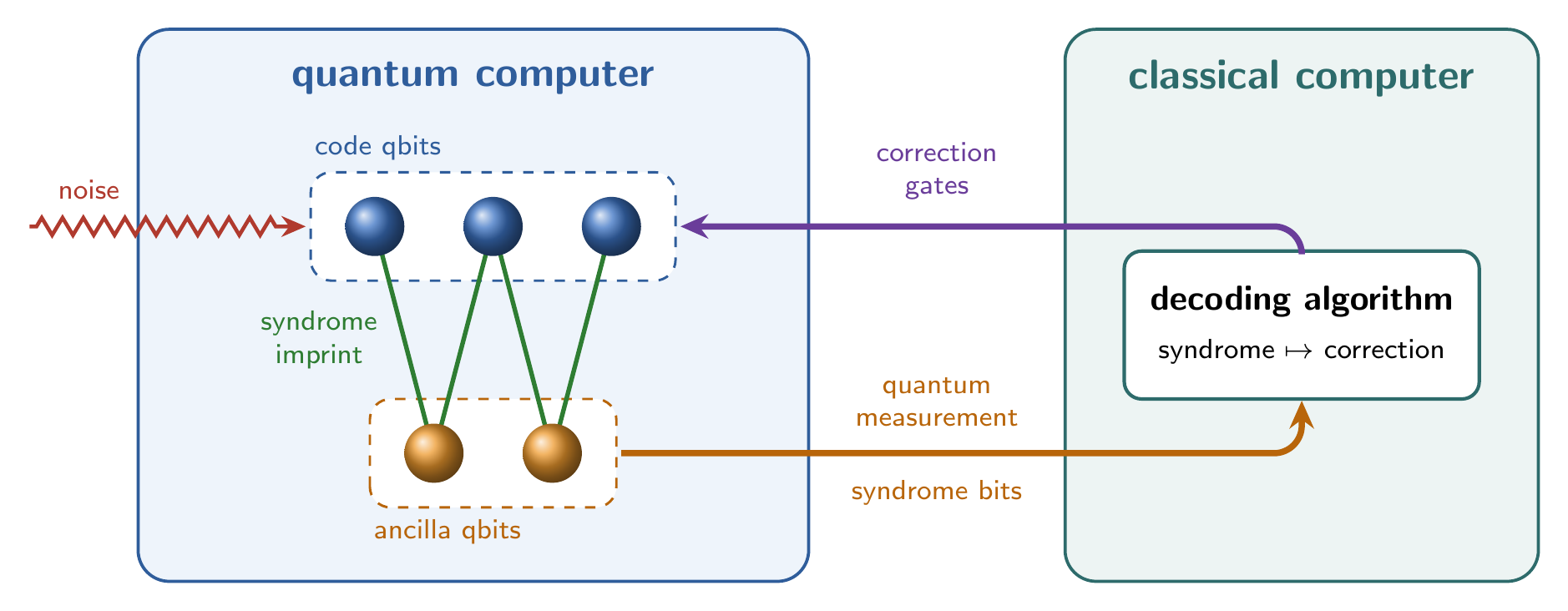
It is a nontrivial and remarkable theoretical insight (involving results such as quantum error threshold theorems) that such a scheme can work
but it remains a substantial engineering challenge to also make it work
In principle
From Ferris & Poulin 2013:
The basic principle of quantum error correction (QEC) is to encode information into the long-range correlations of entangled quantum many-body states in such a way that it cannot be accessed locally. When a local error affects the system, it leaves a detectable imprint—called the error syndrome. The decoding problem consists in inferring the recovery with greatest probability of success given the error syndrome. In general, this is a hard problem, but for well-chosen codes, it can be solved efficiently either exactly or heuristically.
From Steane 06:
Error correction is especially important in quantum computers, because efficient quantum algorithms make use of large scale quantum interference, which is fragile, i.e. sensitive to imprecision in the computer and to unwanted coupling between the computer and the rest of the world. This makes large scale quantum computation so difficult as to be practically impossible unless error correction methods are used. Indeed, before quantum error correction was discovered, it seemed that this fragility would forbid large scale quantum computation. The ability to correct a quantum computer efficiently without disturbing the coherence of the computation is highly non-intuitive, and was thought more or less impossible. The discovery of powerful error correction methods therefore caused much excitement, since it converted large scale quantum computation from a practical impossibility to a possibility.
From Devitt, Nemoto & Munro 2009:
Starting in 1995, several papers appeared, in rapid succession, proposing codes which were appropriate to perform error correction on quantum data (Sho95; Ste96a; CS96; LMPZ96; BSW96). This was a key theoretical development needed to convince the general community that quantum computation was indeed a possibility. Since this initial introduction, the progress in this field has been extensive.
From Zhu & Cross 20:
Although we are currently in an era of quantum computers with tens of noisy qubits, it is likely that a decisive, practical quantum advantage can only be achieved with a scalable, fault-tolerant, error-corrected quantum computer. Therefore, development of quantum error correction is one of the central themes of the next five to ten years.
Within the decade, Google aims to build a useful, error-corrected quantum computer. Our journey to build an error-corrected quantum computer within the decade includes several scientific milestones, including building an error-corrected logical qubit.
Specifically on holographic quantum error correcting codes (see references below):
From Harlow 20:
The codes provided by AdS/CFT often come close to saturating theoretical bounds on the performance of quantum codes. It seems AdS/CFT may be a tool for discovering better quantum cryptography?
holographic codes could be promising candidates to circumvent our results and could possibly realise a universal set of unitary implementations of logical operators.
From CDCW 21:
There are a number of reasons to suspect that holographic codes may be of practical use for quantum computing.
Holographic codes can admit erasure thresholds comparable to that of the widely-studied surface code, and likewise for their threshold against Pauli errors. Their holographic structure also naturally leads to an organization of encoded qubits into a hierarchy of levels of protection from errors, which could be useful for applications which call for many qubits withvarying levels of protection. In particular, this is reminiscent of many schemes for magic state distillation – and indeed, the concatenated codes utilized for magic state distillation share a similar hierarchical structure to holographic codes. The layered structure of holographic codes is also reminiscent of memory architectures in classical computers, where it is useful to have different levels of short- and long-term memory. Although these codes have some notable drawbacks, in particular holographic stabilizer codes require nonlocal stabilizer generators, other codes such as concatenated codes suffer similar drawbacks and have still proven to be useful. Conversely, the stringent requirement of non-local stabilizer generators allows holographic codes to protect many more qubits than a topological code and in fact attain a finite nonzero encoding rate, which is typically not possible for topological codes. Nonetheless, many open questions remain about the usefulness of holographic codes for fault-tolerant quantum computing.
Basic idea of QEC via the 3-qbit code
It is useful and common to illustrate the basic idea of QEC with the 3-qbit code, since it already showcases the key stages of (1.) encoding, (2) syndrome and (3.) correction. But beware that practically relevant code these days are surface codes which are quite different in nature, see also below.
The classical case
Before considering quantum error correction it is useful to step back and briefly reconsider the analogous case of classical error correction.
To set the stage: We regard bit values as elements of the cyclic group of integers modulo 2.
-
Their addition mod 2 is the exclusive or (xor) of bits, denoted
so that is the flip of a bit ,
-
Their multiplication mod 2 is the logical and.
Now, a bit stored or transmitted in a noisy medium may get flipped with some small probability , and error correction is about fixing such flips.
The simplest remedy is redundancy: encode each logical bit by a triple of equal physical bits,
If at most one of the bits in gets flipped, its position in the triple is exactly determined by the following pair of parities:
which vanish exactly on the codewords and . This pair is hence called the error syndrome, since it allows to uniquely identify the position of a one-it flip error (if any), as follows:
Hence classical error correction in this case proceeds by:
-
Syndrome: Measuring the triple state and computing the error syndrome from it.
-
Decoding: Computing from the syndrome the apparent position of the flipped bit according to (2).
-
Correction: Flipping that identified bit back.
This prodedure:
-
succeeds if none or one bit flipped,
-
fails if two or three bits flipped.
Assuming that the bits flip independently of each other, this failure happens with probability
where the factor of 3 counts the choices of the pair of flipped bits. Since , this is smaller than the error probability of an unprotected bit as long as .
A characteristic property of this classical error correction is that the error syndrome is obtained in the most direct way: by reading out, hence by measuring, the state of the tuple of physical bits. Classically, this does no harm, but for qbits this does not work so directly and quantum error correction needs to be a tad more clever than this.
The issue with the quantum case
As we pass from classical bits to quantum bits, qbits, the information to be protected is that of a quantum state of a qbit, encoded by the amplitudes .
The classical triple encoding (1) extends linearly from the canonical linear basis to :
In terms of quantum circuits this operation (3) may be implemented by followed by two CNOT gates (see below).
This (3) is a copying operation, namely of the computational basis states. The no-cloning theorem only rules out that copying be natural (in particular: independent of the choice of basis), which would instead send general to .
A flip of the th qbit now acts as the Pauli operator , hence as
on the th tensor factor and as the identity on the others (with for the error-free case). For example:
Now, applying the classical strategy above verbatim would mean measuring the three qbits in the computational basis. While this would reveal the syndrome, already the first measurement would collapses the quantum state onto one of its two branches (here or , with Born rule probability or , respectively). This would serve to diagnose the error, but would itself destroy the quantum state completely: the amplitudes (the very data to be protected) would be lost.
Notice, however, that the syndrome takes the same value on both branches (here for as well as for ).
To turn this into a quantum observable, consider the Pauli operator
with which the syndrome appears as
This means that each is a joint eigenstate of the syndrome parity observables and , with eigenvalues and , respectively.
Hence while the individual physical bits must not be measured, their parities may.
This motivates adjoining auxiliary ancilla qbits onto which the parities are imprinted by unitary gates. A quantum measurement of just the ancillas is then a measurement on the total system which reveals the syndrome without collapsing the encoded state.
The proper quantum case
Concretely, consider adjoining to the logical Hilbert space two ancilla qbits, hence pass to
and consider on this the imprint unitary operator
(a permutation of the computational basis, implementable by four CNOT gates), which imprints the parities of the code qbits onto ancillas initialized in .
Suppose that the code state has suffered at most one bit flip, so that it is for some unknown . Since the parities agree on both branches of , we have
where is the syndrome of the error in that may be computed from it (2).
Error correction now proceeds in three steps analogous to the classical case above, but replacing code bit measurement by ancilla qbit quantum measurement:
-
Syndrome: Since on the right of (4) we have a product state, measuring only the ancillas yields the syndrome with certainty, while leaving the code qbits in , uncollapsed.
-
Decoding: From the syndrome, a classical algorithm, the decoder, determines , here via the above) syndrome table (2), and thereby chooses the correcting quantum gate .
-
Correction: Applying the chosen correction quantum gate, which restores the code state in case of at most one bit flip error: , since .
This is the 3-qbit bit flip code. Its full quantum circuit reads as follows: encoding, error, syndrome extraction by , measurement, decoding and correction:
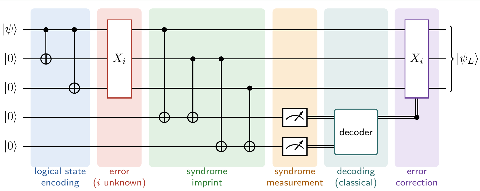
(The final gates are classically controlled (double lines) by the quantum measurement outcomes.)
It should be noted here that the quantum correction mechanism (5) is itself nothing but a quantum circuit, hence, when physically executed, is itself subject to quantum errors. This is a problem that is solved in principle by the quantum error threshold theorems, but in practice it makes this and similar codes actually unusable, see the discussion of Nested codes and Surface codes below.
Refinements
The above bit flip code does not protect against phase flips as reflected by the Pauli operator . These send to , which is again a code state and hence has trivial syndrome under the above code: the error goes undetected and corrupts the logical state.
But since the Hadamard gate
exchanges bit and phase flips, , the same scheme may be run in the Hadamard-transformed basis . Hence the encoding
gives the “3-qbit phase flip code”, with syndrome given by the parity observables and . It corrects any single phase flip, but now not bit flips.
Nesting the two codes, by encoding each of the three qbits of the phase flip code via the bit flip code, yields Shor’s 9-qbit code:
This corrects bit flips, phase flips and their composites on any single qbit. In fact this suffices to correct arbitrary errors on a single qbit. Every operator on a qbit is a linear combination of , , and , and the syndrome measurement collapses such a superposition of errors onto one of its components, which is then corrected as before.
All of these are examples of stabilizer codes: the code space is the joint -eigenspace of a commuting set of products of Pauli operators (for the bit flip code: and ), whose measurement via ancillas yields the error syndrome.
General QEC codes
The simple but important special case of passive correction of erasures may be handled by quantum error correcting codes:
Recall that a classical error correcting code on a finite set of states is, typically, a choice of injection of into some larger finite set, typically a Cartesian power
(often considered in the form of linear codes, but classical nonetheless). In quantum physics the Cartesian product of sets of states is replaced by the tensor product of Hilbert spaces.
For a given Hilbert space of quantum states (finite-dimensional in practice), a quantum error correcting code is a choice of linear embedding (the code subspace) of into a larger Hilbert spaces, often an -fold tensor product of copies of some :
such that the information in in some of the tensor factors can be lost without obstructing the reconstruction of (cf. Rowell & Wang 17, Sec. 3.2.3).
(Often one demands additional properties, such as that a given set of linear operators (quantum observables) acting on are implemented on by combinations of operators that act non-trivially only on some of the tensor factors.)
While this is superficially analogous to a classical error correcting code, the crucial and subtle difference is that quantum error correction codes thus take place in a non-Cartesian symmetric monoidal category. For this reason, effects of quantum entanglement play a paramount role in quantum error correction codes.
In practice
While the quantum error threshold theorem shows that quantum error correction of noisy quantum circuits is possible in principle, the practice of QEC at scale remains a major engineering challenge.
The decoding bottleneck
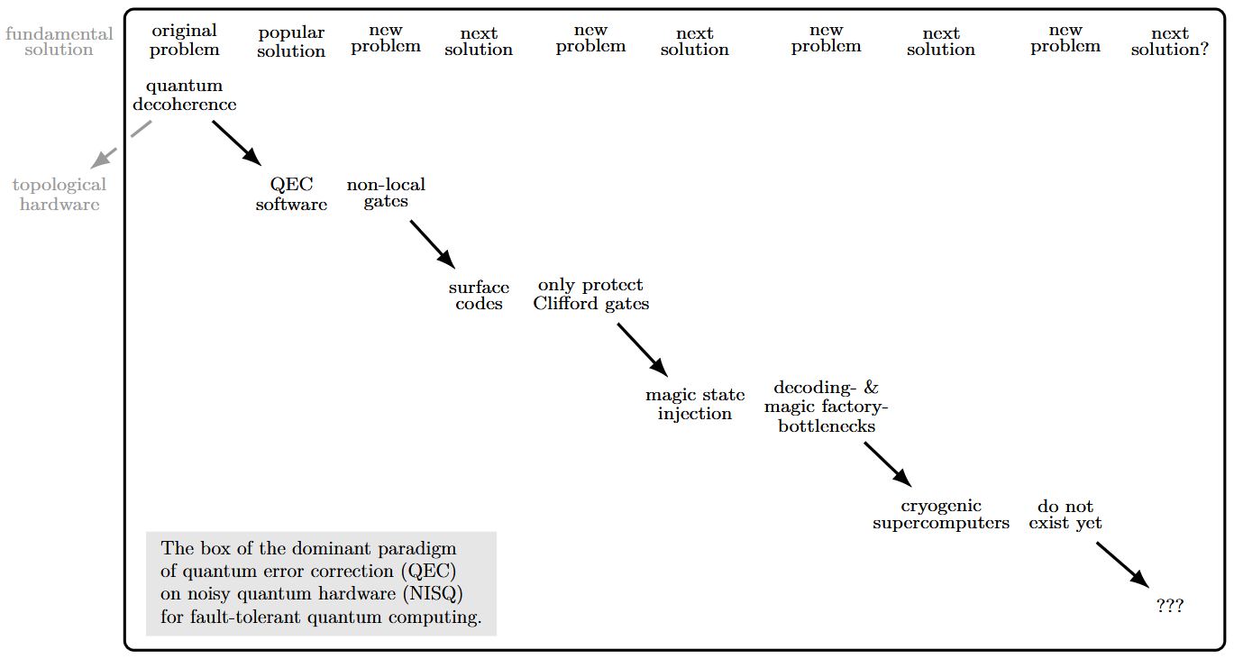
As of the 2020s, quantum error correction (QEC) applied to noisy intermediate-scale quantum (NISQ) machines is the dominant strategy paradigm, in both academia and industry, for potentially achieving meaningful quantum computation in the future.
But in technical discussions, the physical reality of the “endgame” of this approach may be easily missed by outsiders: Even in optimistic scenarios where theoretical error thresholds are achieved, the NISQ+QEC roadmap requires envisioning a staggering future feat of quantum and classical hardware engineering, haunted by intrinsic design tensions.
Namely, the quantum error-correcting mechanism required to run a useful, large-scale application on currently available qubit technology — such as Shor's algorithm (e.g. for cracking RSA-2048 encryption) will involve an astronomical rate of data processing. To maintain the logical quantum state, the auxiliary classical system must measure millions of physical qubits every microsecond, exchanging hundreds of terabytes of error “syndrome” data per second between the quantum device and its classical controller (cf. riverlane 2025). This is a data rate of the order of the global internet traffic! Decoding this torrent of data in real-time requires an amount of classical computational power that exceeds the capabilities of contemporary, building-sized exascale supercomputers (cf. Waintal 2024).
Even if such classical computing power is or were available, standard data cables connecting the quantum chip to an external supercomputer would introduce signal latency exceeding the coherence time of current qubits, rendering the correction commands obsolete upon arrival. Furthermore, the sheer volume of data transfer will or would transmit enormous amounts of thermal noise from the outside world into the quantum machine, jeopardizing its near-zero cooling and its quantum coherence.
This problem is also known as the decoding bottleneck or decoder bottleneck (cf. Mishan 2025, Croot et al. 2025, Ivezic 2026, Mahmud at al. 2026, Canton 2026).
To overcome this formidable scenario, the NISQ+QEC field has now turned to speculating on future classical hardware technology where Application Specific Integrated Circuit (ASICs) hardware is integrated directly into the ultra-cooled quantum refrigerator (e.g., via specialized “Cryo-CMOS” logic; cf. Erol 2026). However, this poses severe thermodynamic contradictions: Standard silicon transistors suffer from carrier freeze-out below , whence one needs to envision an entire new kind of classical computing hardware. More generally, the cooling power at the base of a dilution refrigerator is strictly limited to a few micro-Watts. Therefore, placing a petaflop ASIC chip in near proximity to the quantum device would produce excess heat that under currently understood conditions would destroy the cryogenic environment that the quantum computer relies on.
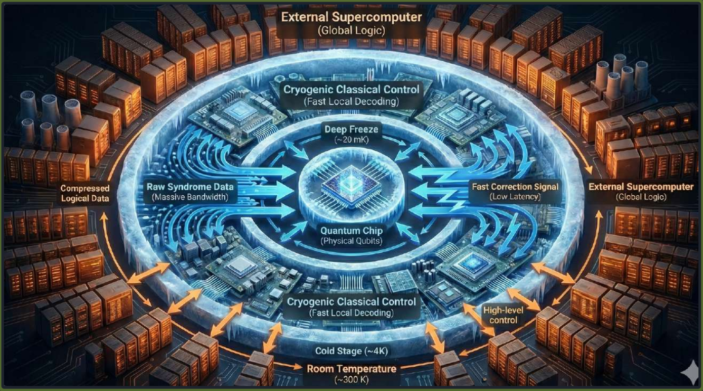
In conclusion, the NISQ+QEC roadmap for achieving meaningful commercial value quantum computers is now tacitly banking on unheard of and intrinsically dubious future progress in classical supercomputing technology — which, assuming it can be brought into existence, would then not be used for contentful computation itself, but would solely serve the task of preventing the memory of a quantum computer from decaying.
Aside: Hardware-level protection
The initial problem at the base of the decoding bottlenck problem above is the instability of current qubit technology (NISQ, see there).
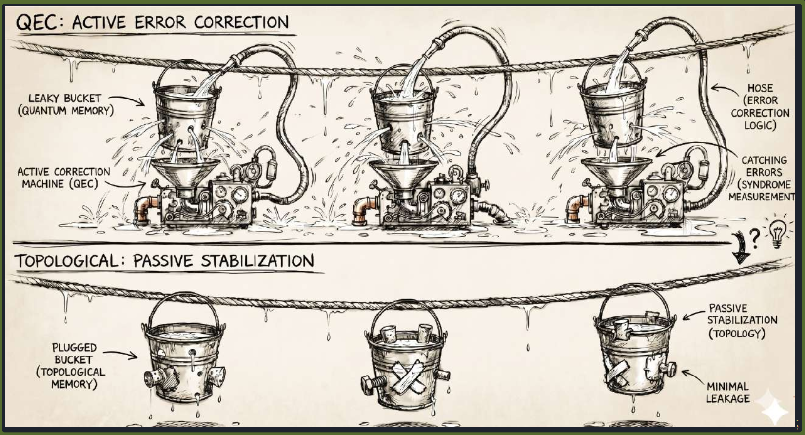
The problem is akin to that of a bucket brigade which operates with extremely leaky buckets. In this picture, the QEC-style solution is like using ever more buckets together with sophisticated machinery that cleverly catches the leaked water only to fill it back into the buckets.
This analogy makes clear that an alternative strategy may be to actually fix the buckets. On the quantum technology side this corresponds to the approach of topological quantum computing (cf. Das Sarma 2022), where it is not runtime software redundancy that stabilizes shaky qubits, but intrinsic physical effects in topological quantum hardware.
However, while such topological stabilization of quantum states and topological protection of quantum gates exists in theory (and even that theory is not well developed at this point) essentially no experience with practical engineering implementation exists to date.
Nested codes and Surface codes
An intrinsic practical problem with QEC implemented via quantum circuits as in the simple 3-qbit code example (5) above is that these quantum circuits are themselves subject to errors, needing themselves another layer of QEC, and so on. This may appear to already lead to an infinite regression problem. Remarkably, the quantum error threshold theorem says that, in principle, a finite depth of nested codes is sufficient for breaking even if the baseline physical error rate is below some threshold (whence the name).
However, nested codes require non-local qbit connectivity on the quantum hardware, which becomes quickly technologically unachievable. For this reason, the nested codes that the theory of the threshold theorem considers are actually useless in practice.
For this reason the community has turned instead to surface codes. These mimic (“simulate”) topological mechanisms of error protection by a lattice of qbits using only local connectivity.
While surface codes solve the non-locality of nested codes, this comes at the cost that they correct errors only in Clifford gates, which are not sufficient for universal quantum computation, leaving non-Clifford gates like T-gates unprotected (see below).
Magic state factories
The decoding bottleneck (above) is only part of the problem of practically implementing QEC at scale.
Namely, with the currently most popular error correcting codes, which are surface codes (above), it is only Clifford gates that are error protected (after solving the decoding bottleneck), while universal quantum computing requires further gate type (such as the T-gate) that remain uncorrected by surface codes.
The now standard strategy to work around this problem, trades the missing gate for a resource quantum state: T-gates are enacted by gate teleportation, consuming magic states via a CNOT, a -measurement and a classically controlled -correction (which are all Clifford operations).
This leads to the further practical problem of equipping the quantum computer with a good supply of magic states, which has become a research field all in itself: “magic state factories”. Current estimates are that “magic state distillation” alone will occupy about 90% of the quantum chip, leaving 10% for actual computation, and that this creates a bottleneck on top of and dwarfing the error correction bottlenect (cf. NKM 2026).
Summary and outlook
References: Practical challenges of QEC
More on the above discussion of practical QEC challenges may be found in the following references, with some quotes highlighted:
-
Sankar Das Sarma: Quantum computing has a hype problem, MIT Technology Review (March 2022)
“The qubit systems we have today are a tremendous scientific achievement, but they take us no closer to having a quantum computer that can solve a problem that anybody cares about. […] What is missing is the breakthrough […] bypassing quantum error correction by using far-more-stable qubits, in an approach called topological quantum computing.”
-
Francesco Battistel et al.: Real-Time Decoding for Fault-Tolerant Quantum Computing: Progress, Challenges and Outlook, Nano Futures 7 032003 (2023) [arXiv:2303.00054, doi:10.1088/2399-1984/aceba6]
-
Xavier Waintal: The Quantum House Of Cards, PNAS 121 1 (2024) e2313269120 [doi:10.1073/pnas.2313269120, arXiv:2312.17570]
-
Lior Mishan: Scalable Quantum Error Correction: Breaking Bottlenecks in Quantum Computing, Quantum Machine Blog (June 2025)
-
riverlane: Quantum Error Correction (2025)
-
Volkan Erol: Quantum Computing is No Longer a Physics Problem. It is a Systems Engineering Nightmare, Medium (Jan 2026) [pdf]
-
X. Croot et al.: Enabling Technologies for Scalable Superconducting Quantum Computing [arXiv:2512.15001 quant-ph]
“The i/o of signal between qubit and control electronics is a central bottleneck to scaling. […] Many proposals for long-term fault-tolerant quantum computing require qubit numbers that are orders of magnitude greater than the capacity of available fridges, even when accounting for densification of components and reduction of thermal loads per qubit. […] The qubit overheads for the best FT-QEC schemes are daunting, and the implementation of decoding on the time-scale of the quantum gates (clock cycle) remains an open challenge in many leading hardware platforms. […] Systems of 100k qubits would demand large fractions of the yearly world production [of Helium] based on naive linear scaling.”
-
Marin Ivezic: The Decoder Bottleneck: The CRQC Challenge Nobody Is Talking About, PostQuantum (April 2026)
“The Capability Nobody Mentioned […] The decoder is the classical computer sitting next to the quantum processor, receiving a continuous stream of error syndrome measurements and determining, in real time, what corrections to apply. […] Without a decoder that can keep pace with the quantum hardware, quantum error correction is an offline statistical exercise, not a fault-tolerant computation. A million qubits without a real-time decoder is a million qubits that cannot compute.
This is the capability dimension that […] is most likely to determine whether a cryptographically relevant quantum computer (CRQC) arrives in 2030 or 2045. It is the classical engineering challenge hiding inside the quantum machine, the piece that connects the quantum physics to the classical computation, and the capability that most threat assessments ignore entirely.
The quantum computing field has trained the public, and by extension the security community, to track one number: how many qubits. Security professionals need a more sophisticated model.
If the decoder cannot keep up with the syndrome stream, a backlog forms. […] The backlog grows exponentially, and eventually the computation fails. This is the “backlog problem,” and it is the reason that decoder speed is not a performance optimization but a hard requirement. A decoder that is 10% too slow does not produce a 10% slower computation. It produces a computation that fails entirely.
The decoder must satisfy three simultaneous requirements. […] Speed, accuracy, and scale. Getting any two of three is tractable. Getting all three simultaneously is the unsolved engineering problem at the center of the CRQC timeline.
[…] Decoding Is Harder Than It Sounds
[For superconducting qbits] the decoder must complete its work within that microsecond to avoid backlog. This is the most demanding timing constraint in the quantum computing stack, and it is why FPGA and ASIC implementations are necessary: software decoders running on conventional CPUs cannot reliably meet microsecond deadlines for codes at the distances required for cryptographic applications. The superconducting decoder challenge is fundamentally a hardware problem. The algorithm must be compiled into dedicated circuitry (FPGA or ASIC) that executes in deterministic time, without the variable-latency interrupts, cache misses, and scheduling jitter that make general-purpose CPUs unsuitable for hard real-time constraints.
[…] The gap between current decoder demonstrations and CRQC requirements is large and precisely quantifiable. […] The progress curve is steep. But the destination […] remains far ahead.“
-
Kris Naudts, Zeynep Koruturk, Donald Harmitt: The Quantum Bottleneck Isn’t Error Correction, It’s the Magic State Factory, Firgun Ventures Insight (July 2026)
-
Mahmud et al.: Decoder Architectures and Computational Bottlenecks in QEC: section IV of: Quantum Error Correction Survey, IEEE Access 14 (Sep 2026) 154233–154277 [doi:10.1109/ACCESS.2026.3737721]
-
Manuel Esparcia Cantos: Decoders: The Quiet Bottleneck of Quantum Error Correction, LinkedIn (8. Oct 2026)
“[Quantum error] correction is a hard computational problem that has to be solved by a classical computer, in real time, faster than the quantum computer produces the next round of errors. This is the decoder, and it is one of the field’s quietest and most underappreciated bottlenecks.
This article is about the problem almost no popular account mentions. Everyone talks about qubits and codes; far fewer talk about the classical machine that has to keep up with them. Yet a fault-tolerant quantum computer is impossible without a decoder that is simultaneously accurate enough to correct the errors and fast enough to do it before the backlog explodes.
[…] In a superconducting machine, a new round of syndrome data arrives roughly every microsecond. If the decoder cannot keep pace, unprocessed syndromes pile up faster than they are cleared, a backlog that grows without bound and eventually makes the computation impossible. This is the decoding bottleneck, and it is as real an obstacle to fault tolerance as qubit quality.
[…] WHY DECODERS DESERVE MORE ATTENTION
The decoder is where a beautiful theory meets an unforgiving stopwatch. All the elegance of stabilizer codes and the guarantee of the threshold theorem assume, quietly, that a decoder exists which is accurate enough and fast enough. That assumption is doing enormous work. A code below threshold with a decoder too slow to keep up is not fault-tolerant in practice, no matter how good the qubits are. The classical co-processor is not a footnote to the quantum computer; it is part of the quantum computer.
[…] There is a genuine tension the field has not fully resolved: the most accurate decoders tend to be the slowest, and the fastest tend to be less accurate. The whole game is beating that trade-off, and the platform that first fields a decoder both accurate enough and fast enough at scale removes one of the last quiet obstacles between below-threshold hardware and a working machine.“
Examples
Specific examples
Bit flip codes
See at bit flip code, and the exposition of the 3-qbit code above.
A 3-qutrit code
The following is a simple illustrative example from Cleve, Gottesman & Lo 99, p. 1-2:
Consider a quantum system with a 3-dimensional space of quantum states:
and consider a code space inside 3 copies of this space given by the following linear map
This code corrects errors consisting of the loss of one of the three copies, in the following sense:
There is a linear operator acting only on two of the three copies, explicitly given (ADH 14 (3.6)) by
such that
The HaPPY code
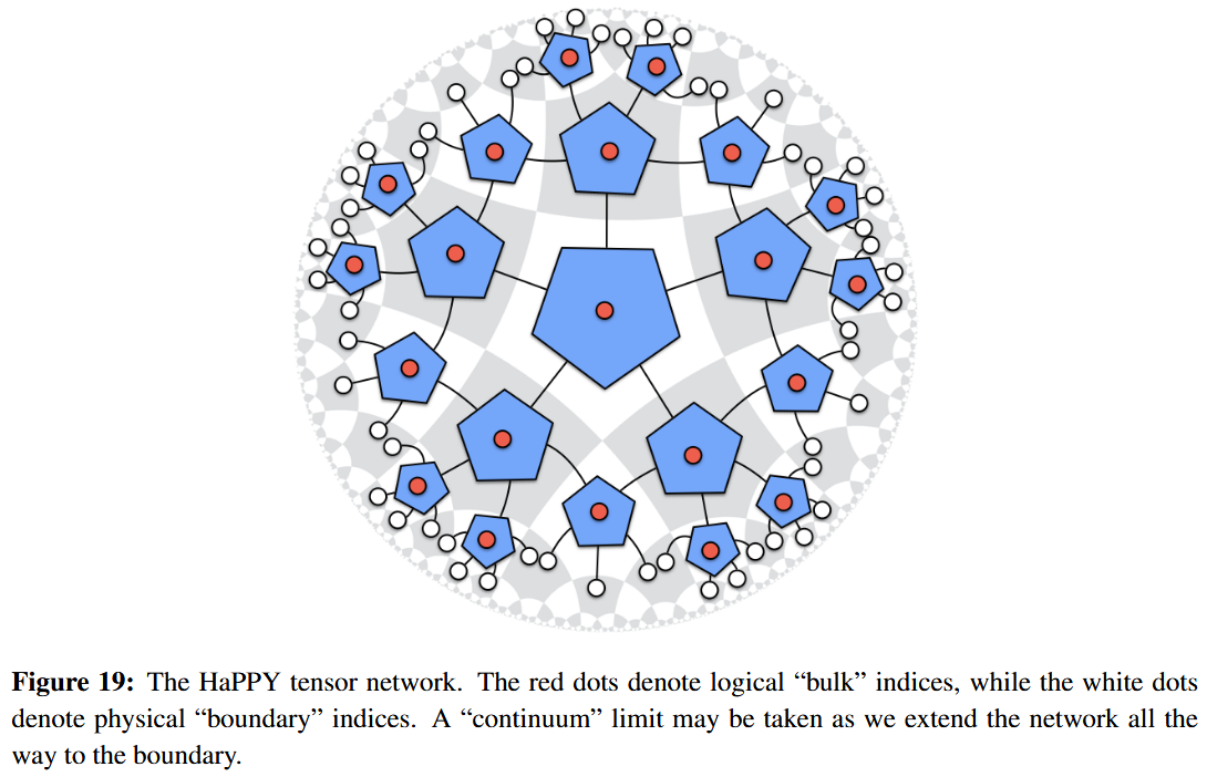
The HaPPY code is a quantum error correction code (a class of such codes really, indexed by a “cutoff” natural number) which is thought to exhibit characteristic properties akin to the encoding of bulk-quantum states by boundary-states expected in the AdS/CFT correspondence. In particular, the HaPPY code (or rather the tensor network that defines it) exhibits a discretized form of the Ryu-Takayanagi formula for holographic entanglement entropy.
Concretely, the the HaPPY code subspace is the image of the linear map formed by:
-
picking a perfect tensor of rank 6;
-
picking a finite cutoff of the pentagonal tesselation of the hyperbolic plane;
-
regarding its Poincaré dual graph as a tensor network (string diagram in finite-dimensional vector spaces) by
-
regarding the uncontracted edges at the cutoff boundary as output (shown in white)
and thus as a linear map from the tensor product over the bulk-vertices to the tensor product over the edges sticking out over the boundary.
Majorana dimer codes
See at Majorana dimer code.
Classes of examples
Related concepts
References
General
The idea of quantum encryption based on the no-cloning theorem originates with:
- Stephen Wiesner, Conjugate Coding, circulated in the 1960s, finally published in ACM SIGACT News 15 1 (1983) 78–88 (original pdf, doi:10.1145/1008908.1008920)
Original articles on quantum error correcting codes:
-
Peter W. Shor, Scheme for reducing decoherence in quantum computer memory, Phys. Rev. A 52, R2493(R) 1995 (doi:10.1103/PhysRevA.52.R2493)
-
Andrew M. Steane, Error Correcting Codes in Quantum Theory, Phys. Rev. Lett. 77, 793 1996 (doi:10.1103/PhysRevLett.77.793)
-
Robert Calderbank, Peter W. Shor, Good Quantum Error-Correcting Codes Exist, Phys. Rev. A, Vol. 54, No. 2, pp. 1098-1106, 1996 (doi:10.1103/PhysRevA.54.1098)
-
Raymond Laflamme, Cesar Miquel, Juan Pablo Paz, Wojciech H. Zurek, Perfect Quantum Error Correction Code, Phys. Rev. Lett., 77:198, 1996 (arXiv:quant-ph/9602019)
-
Charles H. Bennett, David P. DiVincenzo, John A. Smolin, William K. Wootters, Mixed State Entanglement and Quantum Error Correction, Phys. Rev. A54:3824-3851, 1996 (doi:10.1103/PhysRevA.54.3824)
-
Andrew M. Steane, Multiple Particle Interference and Quantum Error Correction, Proc. Roy. Soc. Lond. A452 (1996) 2551 (arXiv:quant-ph/9601029)
-
Emanuel Knill, Raymond Laflamme, A Theory of Quantum Error-Correcting Codes, Phys. Rev. Lett. 84:2525-2528, 2000 (arXiv:quant-ph/9604034)
Realization that quantum error correcting codes could make quantum computation practically feasible (quantum error threshold theorem):
-
Emanuel Knill, Raymond Laflamme, Wojciech H. Zurek, Resilient Quantum Computation: Error Models and Thresholds, Proceedings of the Royal Society A 454 1969 (1998) [arXiv:quant-ph/9702058]
-
John Preskill, Fault-tolerant quantum computation, in: Introduction to Quantum Computation and Information, World Scientific (1998) arXiv:quant-ph/9712048, doi:10.1142/3724
-
John Preskill, Reliable Quantum Computers, Proc. Roy. Soc. Lond. A 454 (1998) 385-410 arXiv:quant-ph/9705031, doi:10.1098/rspa.1998.0167
-
Daniel Gottesman, Theory of fault-tolerant quantum computation, Phys. Rev. A 57 (1998) 127-137 doi:10.1103/PhysRevA.57.127
-
Dorit Aharonov, Michael Ben-Or, Fault-Tolerant Quantum Computation With Constant Error Rate, SIAM J. Comput., 38 4 (2008) 1207–1282 [arXiv:quant-ph/9906129, doi:10.1007/978-3-642-32512-0_31]
-
Daniel Gottesman, Fault-Tolerant Quantum Computation, Physics in Canada 63 4 (2007) 183-189 arXiv:quant-ph/0701112
-
Dorit Aharonov, Michael Ben-Or, Fault-Tolerant Quantum Computation With Constant Error Rate, SIAM J. Comput. 38 4 (2008) 1207–1282 (arXiv:quant-ph/9906129, doi:10.1137/S0097539799359385)
-
Panos Aliferis, Daniel Gottesman, John Preskill, Quantum accuracy threshold for concatenated distance-3 codes, Quant. Inf. Comput. 6 (2006) 97-165 (arXiv:quant-ph/0504218)
-
Earl T. Campbell, Barbara M. Terhal, Christophe Vuillot: Roads towards fault-tolerant universal quantum computation, Nature 549 (2017) 172–179 [doi:10.1038/nature23460, arXiv:1612.07330]
Operator algebraic formulation of quantum error correction:
-
David Kribs, Raymond Laflamme, David Poulin, A Unified and Generalized Approach to Quantum Error Correction, Phys. Rev. Lett. 94, 180501 (2005) (arXiv:quant-ph/0412076)
-
David W. Kribs, Raymond Laflamme, David Poulin, Maia Lesosky, Operator quantum error correction, Quant. Inf. & Comp., 6 (2006), 383-399 (arXiv:quant-ph/0504189)
-
Cédric Bény, Achim Kempf, David W. Kribs, Generalization of Quantum Error Correction via the Heisenberg Picture, Phys. Rev. Lett. 98, 100502 – Published 7 March 2007 (doi:10.1103/PhysRevLett.98.100502, arXiv:quant-ph/0608071)
-
Cédric Bény, Achim Kempf, David W. Kribs, Quantum Error Correction of Observables, Phys. Rev. A 76, 042303 (2007) (arXiv:0705.1574)
Introduction and survey:
-
Alexei Kitaev, Quantum computations: algorithms and error correction, Russian Mathematical Surveys, 52 6 (1997) [doi:10.1070/RM1997v052n06ABEH002155, pdf]
-
Michael A. Nielsen, Isaac L. Chuang, Chapter 10 of: Quantum computation and quantum information, Cambridge University Press (2000) [doi:10.1017/CBO9780511976667, pdf, pdf]
-
Simeon Ball, Aina Centelles, Felix Huber, Quantum error-correcting codes and their geometries (arXiv:2007.05992)
-
Andrew M. Steane, A Tutorial on Quantum Error Correction, in: Proceedings of the International School of Physics “Enrico Fermi”, course CLXII, “Quantum Computers, Algorithms and Chaos” (2006) [pdf, pdf]
-
Daniel Gottesman: An Introduction to Quantum Error Correction and Fault-Tolerant Quantum Computation, in: Quantum Information Science and Its Contributions to Mathematics, Proceedings of Symposia in Applied Mathematics 68 (2010) [arXiv:0904.2557, doi:10.1090/psapm/068]
-
Isaac L. Chuang, Quantum error correction, Chapter 7 in: Quantum Machines: Measurement and Control of Engineered Quantum Systems Lecture Notes of the Les Houches Summer School 96 (2011) 273–320 [doi:10.1093/acprof:oso/9780199681181.003.0007]
-
Simon J. Devitt, Kae Nemoto, William J. Munro, Quantum Error Correction for Beginners, Rep. Prog. Phys. 76 (2013) 076001 [arXiv:0905.2794, doi:10.1088/0034-4885/76/7/076001]
-
Daniel A. Lidar, Todd A. Brun (eds.): Quantum Error Correction, Cambridge University Press (2013) [ISBN:9780521897877, doi:10.1017/CBO9781139034807]
-
Héctor Bombín: An Introduction to Topological Quantum Codes, in: Quantum Error Correction, Cambridge University Press (2013) [ISBN:9780521897877, arxiv:1311.0277]
-
Eric Rowell, Zhenghan Wang, Section 3.2.3 of: Mathematics of Topological Quantum Computing, Bull. Amer. Math. Soc. 55 (2018), 183-238 (arXiv:1705.06206, doi:10.1090/bull/1605)
-
Scott Aaronson, Chapter 27 of: Introduction to Quantum Information Science (2018) [pdf, webpage]
-
Joschka Roffe, Quantum Error Correction: An Introductory Guide, Contemporary Physics 2019 (arXiv:1907.11157)
-
Bei Zeng, Xie Chen, Duan-Lu Zhou, Xiao-Gang Wen:
Sec. 3 of: Quantum Information Meets Quantum Matter – From Quantum Entanglement to Topological Phases of Many-Body Systems, Quantum Science and Technology (QST), Springer (2019) arXiv:1508.02595, doi:10.1007/978-1-4939-9084-9
-
Guanyu Zhu, Andrew Cross, Hardware-aware approach for fault-tolerant quantum computation, IBM Research Blog, September 2, 2020
-
Priya J. Nadkarni, Narayanan Rengaswamy, Bane Vasić: Tutorial on Quantum Error Correction for 2024 Quantum Information Knowledge (QuIK) Workshop [arXiv:2407.12737, inSpire:2808724]
See also:
-
Wikipedia, Quantum error correction
-
Victor V. Albert, Philippe Faist: Handbook of Error-Correcting Codes [arXiv:2606.11484]
In the context of quantum secret sharing:
- Richard Cleve, Daniel Gottesman, Hoi-Kwong Lo, How to share a quantum secret, Phys. Rev. Lett. 83 (1999) 648-651 (arXiv:quant-ph/9901025)
In the context of quantum communication:
- Matthias Christandl, Alexander Müller-Hermes, Fault-tolerant Coding for Quantum Communication,
IEEE Transactions on Information Theory, [arXiv:2009.07161 doi:10.1109/TIT.2022.3169438]
On (in-)compatibility of quantum error correction with universality of quantum gates (Eastin-Knill theorem):
-
Bryan Eastin, Emanuel Knill, Restrictions on Transversal Encoded Quantum Gate Sets, Phys. Rev. Lett. 102, 110502 (2009) (arXiv:0811.4262)
-
Paul Webster, Michael Vasmer, Thomas R. Scruby, Stephen D. Bartlett, Universal Fault-Tolerant Quantum Computing with Stabiliser Codes (arXiv:2012.05260)
For quantum annealing processes:
- Kristen L. Pudenz, Tameem Albash, Daniel A. Lidar: Error-corrected quantum annealing with hundreds of qubits, Nature Communications 5 3243 (2014) [doi:10.1038/ncomms4243]
On continuous variable quantum codes:
-
Samuel L. Braunstein, Peter van Loock, §IV.C in: Quantum information with continuous variables, Rev. Mod. Phys. 77 2 (2005) 513 [arXiv:quant-ph/0410100, doi:10.1103/RevModPhys.77.513]
-
Samuel L. Braunstein, Arun K. Pati, Quantum Information with Continuous Variables, Springer (2003) [doi:10.1007/978-94-015-1258-9]
-
Allan D. C. Tosta, Thiago O. Maciel, Leandro Aolita, Grand Unification of continuous-variable codes [arXiv:2206.01751]
In relation to the SYK model:
- Shao-Kai Jian, Chunxiao Liu, Xiao Chen, Brian Swingle, Pengfei Zhang, Quantum error as an emergent magnetic field (arXiv:2106.09635)
In relation to continuous symmetries:
- Zi-Wen Liu, Sisi Zhou, Approximate symmetries and quantum error correction (arXiv:2111.06355)
Further developments:
- Mackenzie H. Shaw, Andrew C. Doherty, Arne L. Grimsmo, Stabilizer subsystem decompositions for single- and multi-mode Gottesman-Kitaev-Preskill codes [arXiv:2210.14919]
On relevant classical control mechanisms:
-
Hideo Mabuchi, Continuous quantum error correction as classical hybrid control, New J. Phys. 11 (2009) 105044 [doi:10.1088/1367-2630/11/10/105030]
-
Alexandru Paler, Daniel Herr, Simon J. Devitt, Really Small Shoe Boxes - On Realistic Quantum Resource Estimation, Computer 52 6 (2019) [arXiv:1902.08104, doi:10.1109/MC.2019.2908621]
In relation to the Penrose tiling:
- Zhi Li, Latham Boyle, The Penrose Tiling is a Quantum Error-Correcting Code [arXiv:2311.13040]
Relating quantum error correction to linear logic:
- Daniel Murfet, William Troiani, Linear Logic and Quantum Error Correcting Codes [arXiv:2405.19051]
Experimental realization
Realization of quantum error correction in experiment, hence in actual quantum computers:
-
D. G. Cory, M. D. Price, W. Maas, Emanuel Knill, Raymond Laflamme, Wojchiek H. Zurek, T. F. Havel, and S. S. Somaroo, Experimental Quantum Error Correction, Phys. Rev. Lett. 81, 2152 (1998) (doi:10.1103/PhysRevLett.81.2152)
-
Daniel Nigg, Markus Mueller, Esteban A. Martinez, Philipp Schindler, Markus Hennrich, Thomas Monz, Miguel A. Martin-Delgado, Rainer Blatt,
Experimental Quantum Computations on a Topologically Encoded Qubit, Science 18 Jul 2014: Vol. 345, Issue 6194, pp. 302-305 (arXiv:1403.5426, doi:10.1126/science.1253742)
(via methods from topological quantum computation)
-
Adrian Cho, The biggest flipping challenge in quantum computing, Science News Jul. 9, 2020
(exposition)
-
Y. Ma et al. Error-transparent operations on a logical qubit protected by quantum error correction, Nature Physics volume 16, pages 827–831 (2020) (doi:10.1038/s41567-020-0893-x)
-
Ming Gong et al. Experimental exploration of five-qubit quantum error correcting code with superconducting qubits, National Science Review, nwab011 (2021) (doi:10.1093/nsr/nwab011)
survey in:
EurekaAlert, Science China Press: Demonstration of the universal quantum error correcting code with superconducting qubits, March 2021 (2021-03/scp-dot031521)
-
Erik Lucero (Google), Unveiling our new Quantum AI campus, May 18, 2021
(outlook)
-
Th. Monz et al., Demonstration of fault-tolerant universal quantum gate operations, Nature 605 (2022) 675–680 [doi:10.1038/s41586-022-04721-1]
-
Markus Müller, Andreas Wallraff et al., Realizing Repeated Quantum Error Correction in a Distance-Three Surface Code, Nature 605 (2022) 669–674 [arXiv:2112.03708, doi:10.1038/s41586-022-04566-8]
-
Markus Müller et al., Demonstration of fault-tolerant universal quantum gate operations, Nature 605 (2022) 675-680 [doi:10.1038/s41586-022-04721-1, arXiv:2111.12654]
-
Google Quantum AI et al.: Quantum error correction below the surface code threshold, Nature 638 (2025) 920-926 [doi:10.1038/s41586-024-08449-y, arXiv:2408.13687]
Via holographic tensor networks
First quantum error correcting codes associated with planar bulk/boundary systems:
-
S. B. Bravyi, Alexei Kitaev, Quantum codes on a lattice with boundary (arXiv:quant-ph/9811052)
-
Michael Freedman, David A. Meyer, Projective Plane and Planar Quantum Codes, Found. Comput. Math. 1, 325–332 (2001) (arXiv:quant-ph/9810055, doi:10.1007/s102080010013)
First suggestion relating quantum error correction to black hole entropy:
- Erik Verlinde, Herman Verlinde, Black Hole Entanglement and Quantum Error Correction, J. High Energ. Phys. 2013, 107 (2013) (arXiv:1211.6913, doi:10.1007/JHEP10(2013)107)
Introducing the idea of quantum error correcting codes given by tensor network states:
-
Andrew J. Ferris, David Poulin, Tensor Networks and Quantum Error Correction, Phys. Rev. Lett. 113, 030501 (2014) (arXiv:1312.4578)
-
Dave Bacon, Steven T. Flammia, Aram W. Harrow, Jonathan Shi, Sparse Quantum Codes from Quantum Circuits, Proc. of STOC ‘15, pp. 327-334 (2015); IEEE Transactions on Information Theory, vol 63, no 4, pp 2464-2479, April 2017 (arXiv:1411.3334)
following observations in
-
Brian Swingle, Entanglement Renormalization and Holography, Phys. Rev. D 86, 065007 (2012) (arXiv:0905.1317)
-
Brian Swingle, Constructing holographic spacetimes using entanglement renormalization (arXiv:1209.3304, spire:1185813)
Interpretation of holographic tensor networks encoding holographic entanglement entropy in models for AdS2-CFT1 duality as quantum error correcting codes:
-
Ahmed Almheiri, Xi Dong, Daniel Harlow, Bulk Locality and Quantum Error Correction in AdS/CFT, JHEP 1504:163,2015 (arXiv:1411.7041, doi:10.1007/JHEP04(2015)163)
(using Bény-Kempf-Kribs 06)
with precursor observations in
-
Beni Yoshida, Information storage capacity of discrete spin systems, Annals of Physics 338, 134 (2013) (arXiv:1111.3275)
(focus on classical error correcting codes)
-
Jose I. Latorre, German Sierra, Holographic codes (arXiv:1502.06618)
and concrete implementation by the HaPPY code:
- Fernando Pastawski, Beni Yoshida, Daniel Harlow, John Preskill, Holographic quantum error-correcting codes: Toy models for the bulk/boundary correspondence, JHEP 06 (2015) 149 (arXiv:1503.06237)
and possibly more generally:
- Daniel Harlow, The Ryu–Takayanagi Formula from Quantum Error Correction, Comm. Math. Phys. 354 (2017) 865–912 [doi:10.1007/s00220-017-2904-z, arXiv:1607.03901]
Introduction of the more general Majorana dimer code:
- Alexander Jahn, Marek Gluza, Fernando Pastawski, Jens Eisert, Majorana dimers and holographic quantum error-correcting codes, Phys. Rev. Research 1, 033079 (2019) (arXiv:1905.03268)
Exposition and review:
-
John Preskill, Is spacetime a quantum error-correcting code?, talk at KITP 2015 (pdf, pdf)
-
Daniel Harlow, TASI Lectures on the Emergence of Bulk Physics in AdS/CFT, PoS TASI2017 (2018) 002 (arXiv:1802.01040, doi:10.22323/1.305.0002)
-
Pratik Rath, Aspects of Holography And Quantum Error Correction, 2020 (pdf, pdf)
-
Melanie Swan, Renato P dos Santos, Frank Witte, The AdS/CFT Correspondence and Holographic Codes (doi:10.1142/9781786348210_0013, doi:10.1142/9781786348210_0014), Part 5 in: Between Science and Economics, Volume 2: Quantum Computing Physics, Blockchains, and Deep Learning Smart Networks, World Scientific 2020 (doi:10.1142/q0243)
-
Daniel Harlow, Computation and Holography, talk at Snowmass Computational Frontier Workshop 2020 (pdf, pdf)
-
Alexander Jahn, Jens Eisert, Holographic tensor network models and quantum error correction: A topical review (arXiv:2102.02619)
-
Tanay Kibe, Prabha Mandayam, Ayan Mukhopadhyay, Holographic spacetime, black holes and quantum error correcting codes: A review (arXiv:2110.14669)
Further discussion of holographic quantum error correcting codes:
-
Henrique Lazari, Reginaldo Palazzo Jr., Geometrically uniform hyperbolic codes, Comput. Appl. Math. vol.24 no.2 Petrópolis 2005 (doi:10.1590/S0101-82052005000200002)
-
Enrico M. Brehm, Benedikt Richter, Classical Holographic Codes, Phys. Rev. D 96, 066005 (2017) (arXiv:1609.03560)
-
Fernando Pastawski, John Preskill, Code properties from holographic geometries, Phys. Rev. X 7, 021022 (2017) (arXiv:1612.00017)
-
Robert J. Harris, Nathan A. McMahon, Gavin K. Brennen, Thomas M. Stace, Calderbank-Steane-Shor Holographic Quantum Error Correcting Codes, Phys. Rev. A 98, 052301 (2018) (arXiv:1806.06472)
-
Tamara Kohler, Toby Cubitt, Toy Models of Holographic Duality between local Hamiltonians, J. High Energy Phys. 2019:17 (2019) (arXiv:1810.08992)
-
Tobias J. Osborne, Deniz E. Stiegemann, Dynamics for holographic codes, J. High Energ. Phys. 2020, 154 (2020) (arXiv:1706.08823)
-
Martina Gschwendtner, Robert König, Burak Şahinoğlu & Eugene Tang, Quantum error-detection at low energies, Journal of High Energy Physics volume 2019, Article number: 21 (2019) (arXiv:1902.02115)
-
Nathan A. McMahon, Gavin K. Brennen, Thomas M. Stace, Robert J. Harris, Elliot Coupe, Decoding Holographic Codes with an Integer Optimisation Decoder (arXiv:2008.10206)
-
Terry Farrelly, Robert J. Harris, Nathan A. McMahon, Thomas M. Stace, Tensor-network codes (arXiv:2009.10329)
-
ChunJun Cao, Brad Lackey, Approximate Bacon-Shor Code and Holography (arXiv:2010.05960)
-
Sam Cree, Kfir Dolev, Vladimir Calvera, Dominic J. Williamson, Fault-tolerant logical gates in holographic stabilizer codes are severely restricted (arXiv:2103.13404)
-
Robert de Mello Koch, Eunice Gandote, Nirina Hasina Tahiridimbisoa, Hendrik J.R. Van Zyl, Quantum Error Correction and Holographic Information from Bilocal Holography (arXiv:2106.00349)
-
Chris Akers, Geoff Penington, Quantum minimal surfaces from quantum error correction (arXiv:2109.14618)
-
ChunJun Cao, Brad Lackey, Quantum Lego: Building Quantum Error Correction Codes from Tensor Networks, PRX Quantum 3 020332 (2022) arXiv:2109.08158, doi:10.1103/PRXQuantum.3.020332
-
Jason Pollack, Patrick Rall, Andrea Rocchetto, Understanding holographic error correction via unique algebras and atomic examples, Journal of High Energy Physics, 56 (2022) arXiv:2110.14691
-
Dmitry S. Ageev, Exploring uberholography [arXiv:2208.07387]
-
Matthew Steinberg, Sebastian Feld, Alexander Jahn, Holographic Codes from Hyperinvariant Tensor Networks [arXiv:2304.02732]
Understanding in terms of the eigenstate thermalization hypothesis:
- Ning Bao, Newton Cheng, Eigenstate Thermalization Hypothesis and Approximate Quantum Error Correction, JHEP 08 (2019) 152 (arXiv:1906.03669)
In relation to holographic Renyi entropy:
- Chris Akers, Pratik Rath, Holographic Renyi entropy from quantum error correction, J. High Energ. Phys. 2019, 52 (2019) (arXiv:1811.05171)
From tesselations of higher-dimensional hyperbolic space:
- Vivien Londe, Anthony Leverrier, Golden codes: quantum LDPC codes built from regular tessellations of hyperbolic 4-manifolds (arXiv:1712.08578)
In view of black hole thermodynamics:
-
Ahmed Almheiri, Holographic Quantum Error Correction and the Projected Black Hole Interior (arXiv:1810.02055)
-
Isaac H. Kim, Eugene Tang, John Preskill, The ghost in the radiation: Robust encodings of the black hole interior, JHEP 2020, 31 (2020) (arXiv:2003.05451)
-
Chris Akers, Netta Engelhardt, Daniel Harlow, Geoff Penington, Shreya Vardhan, The black hole interior from non-isometric codes and complexity [arXiv:2207.06536]
-
Daniel Harlow, A theory of the black hole interior, talk at Strings 2022 [indico:4940817/]
Discussion of gauge symmetry of holographic tensor networks and their quantum error correcting codes:
- Kfir Dolev, Vladimir Calvera, Sam Cree, Dominic J. Williamson, Gauging the bulk: generalized gauging maps and holographic codes (arXiv:2108.11402)
Relation of quantum error correcting codes to the Monster vertex operator algebra and more generally to 2d SCFT and string theory:
- Jeffrey A. Harvey, Gregory W. Moore, Moonshine, Superconformal Symmetry, and Quantum Error Correction, J. High Energ. Phys. 2020, 146 (2020). (arXiv:2003.13700)
In relation to the large N limit:
- Alexey Milekhin, Quantum error correction and large (arXiv:2008.12869)
In relation to renormalization group flow:
- Keiichiro Furuya, Nima Lashkari, Mudassir Moosa, Renormalization group and approximate error correction (arXiv:2112.05099)
In relation to fixed-point path integrals:
- Andreas Bauer, Topological error correcting processes from fixed-point path integrals (arXiv:2303.16405)
Musings on possible implications on relations between quantum gravity and quantum information:
-
Simons Foundation, It from Qubit: Simons Collaboration on Quantum Fields, Gravity and Information
-
Iulia Georgescu, Strings and qubits, Nature Reviews Physics volume 1, page 477 (2019) (doi:s42254-019-0087-6)
-
Natalie Wolchover, How Space and Time Could Be a Quantum Error-Correcting Code, Quanta Magazine, Jan. 3 2019
-
Tom Banks, Holographic Space-time and Quantum Information (arXiv:2001.08205)
-
ChunJun Cao, From Quantum Codes to Gravity: A Journey of Gravitizing Quantum Mechanics (arXiv:2112.00199)
-
Takaaki Kuwahara, Ryota Nasu, Gota Tanaka, Asato Tsuchiya: Quantum error correction realized by the renormalization group in scalar field theories [arXiv:2401.17795]
Last revised on November 5, 2026 at 11:09:27. See the history of this page for a list of all contributions to it.