nLab geometry of physics -- perturbative quantum field theory
These notes (pdf, 323 pages) mean to give an expository but rigorous introduction to the basic concepts of relativistic perturbative quantum field theories, specifically those that arise as the perturbative quantization of Lagrangian field theories – such as quantum electrodynamics, quantum chromodynamics, and perturbative quantum gravity appearing in the standard model of particle physics.
This is one chapter of geometry of physics.
Previous chapters: smooth sets, supergeometry.
Contents
For broad introduction of the idea of the topic of perturbative quantum field theory see there and see
- PhysicsForums-Insights: Introduction to Perturbative Quantum Field Theory
Here, first we consider classical field theory (or rather pre-quantum field theory), complete with BV-BRST formalism; then its deformation quantization via causal perturbation theory to perturbative quantum field theory. This mathematically rigorous (i.e. clear and precise) formulation of the traditional informal lore has come to be known as perturbative algebraic quantum field theory.
We aim to give a fully local discussion, where all structures arise on the “jet bundle over the field bundle” (introduced below) and “transgress” from there to the spaces of field histories over spacetime (discussed further below). This “Higher Prequantum Geometry” streamlines traditional constructions and serves the conceptualization in the theory. This is joint work with Igor Khavkine.
In full beauty these concepts are extremely general and powerful; but the aim here is to give a first precise idea of the subject, not a fully general account. Therefore we concentrate on the special case where spacetime is Minkowski spacetime (def. below), where the field bundle (def. below) is an ordinary trivial vector bundle (example below) and hence the Lagrangian density (def. below) is globally defined. Similarly, when considering gauge theory we consider just the special case that the gauge parameter-bundle is a trivial vector bundle and we concentrate on the case that the gauge symmetries are “closed irreducible” (def. below). But we aim to organize all concepts such that the structure of their generalization to curved spacetime and non-trivial field bundles is immediate.
This comparatively simple setup already subsumes what is considered in traditional texts on the subject; it captures the established perturbative BRST-BV quantization of gauge fields coupled to fermions on curved spacetimes – which is the state of the art. Further generalization, necessary for the discussion of global topological effects, such as instanton configurations of gauge fields, will be discussed elsewhere (see at homotopical algebraic quantum field theory).
Alongside the theory we develop the concrete examples of the real scalar field, the electromagnetic field and the Dirac field; eventually combining these to a disussion of quantum electrodynamics.
running examples
| field | field bundle | Lagrangian density | equation of motion |
|---|---|---|---|
| real scalar field | expl. | expl. | expl. |
| Dirac field | expl. | expl. | expl. |
| electromagnetic field | expl. | expl. | expl. |
| Yang-Mills field | expl. , expl. | expl. | expl. |
| B-field | expl. | expl | expl. |
| field | Poisson bracket | causal propagator | Wightman propagator | Feynman propagator |
|---|---|---|---|---|
| real scalar field | expl. , expl. | prop. | def. | def. |
| Dirac field | expl. , expl. | prop. | def. | def. |
| electromagnetic field | prop. | prop. |
| field | gauge symmetry | local BRST complex | gauge fixing |
|---|---|---|---|
| electromagnetic field | expl. | expl. | expl. |
| Yang-Mills field | expl. | expl. | … |
| B-field | expl. | expl. | … |
| interacting field theory | interaction Lagrangian density | interaction Wick algebra-element |
|---|---|---|
| phi^n theory | exp. | expl. |
| quantum electrodynamics | expl. | expl. |
References
Pointers to the literature are given in each chapter, alongside the text. The following is a selection of these references.
The discussion of spinors in chapter 2. Spacetime follows Baez-Huerta 09.
The functorial geometry of supergeometric spaces of field histories in 3. Fields follows Schreiber 13, further developed by Giotopoulos & Sati 2023.
For the jet bundle-formulation of variational calculus of Lagrangian field theory in 4. Field variations, and 5. Lagrangians we follow Anderson 89 and Olver 86, further developed by Giotopoulos & Sati 2023; for 6. Symmetries augmented by Fiorenza-Rogers-Schreiber 13b.
The identification of polynomial observables with distributions in 7. Observables was observed by Paugam 12.
The discussion of the Peierls-Poisson bracket in 8. Phase space is based on Khavkine 14.
The derivation of wave front sets of propagators in 9. Propagators takes clues from Radzikowski 96 and uses results from Gelfand-Shilov 66.
For the general idea of BV-BRST formalism a good review is Henneaux 90.
The Lie algebroid-perspective on BRST complexes developed in chapter 10. Gauge symmetries, may be compared to Barnich 10.
For the local BV-BRST theory laid out in chapter 11. Reduced phase space we are following Barnich-Brandt-Henneaux 00.
For the BV-gauge fixing developed in 12. Gauge fixing we take clues from Fredenhagen-Rejzner 11a.
For the free quantum BV-operators in 13. Free quantum fields and the interacting quantum master equation in 15. Interacting quantum fields we are following Fredenhagen-Rejzner 11b, Rejzner 11, which in turn is taking clues from Hollands 07.
The discussion of quantization in 13. Quantization takes clues from Hawkins 04, Collini 16 and spells out the derivation of the Moyal star product from geometric quantization of symplectic groupoids due to Gracia-Bondia & Varilly 94.
The perspective on the Wick algebra in 14. Free quantum fields goes back to Dito 90 and was revived for pAQFT in Dütsch-Fredenhagen 00. The proof of the folklore result that the perturbative Hadamard vacuum state on the Wick algebra is indeed a state is cited from Dütsch 18.
The discussion of causal perturbation theory in 15. Interacting quantum fields follows the original Epstein-Glaser 73. The relevance here of the star product induced by the Feynman propagator was highlighted in Fredenhagen-Rejzner 12. The proof that the interacting field algebra of observables defined by Bogoliubov's formula is a causally local net in the sense of the Haag-Kastler axioms is that of Brunetti-Fredenhagen 00.
Our derivation of Feynman diagrammatics follows Keller 10, chapter IV, our derivation of the quantum master equation follows Rejzner 11, section 5.1.3, and our discussion of Ward identities is informed by Dütsch 18, chapter 4.
In chapter 16. Renormalization we take from Brunetti-Fredenhagen 00 the perspective of Epstein-Glaser renormalization via extension of distributions and from Brunetti-Dütsch-Fredenhagen 09 and Dütsch 10 the rigorous formulation of Gell-Mann Low renormalization group flow, UV-regularization, effective quantum field theory and Polchinski's flow equation.
Acknowledgement
These notes profited greatly from discussions with Igor Khavkine and Michael Dütsch.
Thanks also to Marco Benini, Klaus Fredenhagen, Arnold Neumaier and Kasia Rejzner for helpful discussion.
Geometry
The geometry of physics is differential geometry. This is the flavor of geometry which is modeled on Cartesian spaces with smooth functions between them. Here we briefly review the basics of differential geometry on Cartesian spaces.
In principle the only background assumed of the reader here is
-
usual naive set theory (e.g. Lawvere-Rosebrugh 03);
-
the concept of the continuum: the real line , the plane , etc.
-
the concepts of differentiation and integration of functions on such Cartesian spaces;
hence essentially the content of multi-variable differential calculus.
We now discuss:
As we uncover Lagrangian field theory further below, we discover ever more general concepts of “space” in differential geometry, such as smooth manifolds, diffeological spaces, infinitesimal neighbourhoods, supermanifolds, Lie algebroids and super Lie ∞-algebroids. We introduce these incrementally as we go along:
more general spaces in differential geometry introduced further below
| higher differential geometry | |||||||||||
|---|---|---|---|---|---|---|---|---|---|---|---|
| differential geometry | smooth manifolds (def. ) | diffeological spaces (def. ) | smooth sets (def. ) | formal smooth sets (def. ) | super formal smooth sets (def. ) | super formal smooth ∞-groupoids (not needed in fully perturbative QFT) | |||||
| infinitesimal geometry, Lie theory | infinitesimally thickened points (def. ) | superpoints (def. ) | Lie ∞-algebroids (def. ) | ||||||||
| higher Lie theory | |||||||||||
| needed in QFT for: | spacetime (def. ) | space of field histories (def. ) | Cauchy surface (def. ), perturbation theory (def. ) | Dirac field (expl. ), Pauli exclusion principle | infinitesimal gauge symmetry/BRST complex (expl. ) |
Abstract coordinate systems
What characterizes differential geometry is that it models geometry on the continuum, namely the real line , together with its Cartesian products , regarded with its canonical smooth structure (def. below). We may think of these Cartesian spaces as the “abstract coordinate systems” and of the smooth functions between them as the “abstract coordinate transformations”.
We will eventually consider below much more general “smooth spaces” than just the Cartesian spaces ; but all of them are going to be understood by “laying out abstract coordinate systems” inside them, in the general sense of having smooth functions mapping a Cartesian space smoothly into them. All structure on generalized smooth spaces is thereby reduced to compatible systems of structures on just Cartesian spaces, one for each smooth “probe” . This is called “functorial geometry”.
Notice that the popular concept of a smooth manifold (def./prop. below) is essentially that of a smooth space which locally looks just like a Cartesian space, in that there exist sufficiently many which are (open) isomorphisms onto their images. Historically it was a long process to arrive at the insight that it is wrong to fix such local coordinate identifications , or to have any structure depend on such a choice. But it is useful to go one step further:
In functorial geometry we do not even focus attention on those that are isomorphisms onto their image, but consider all “probes” of by “abstract coordinate systems”. This makes differential geometry both simpler as well as more powerful. The analogous insight for algebraic geometry is due to Grothendieck 65; it was transported to differential geometry by Lawvere 67.
This allows to combine the best of two superficially disjoint worlds: On the one hand we may reduce all constructions and computations to coordinates, the way traditionally done in the physics literature; on the other hand we have full conceptual control over the coordinate-free generalized spaces analyzed thereby. What makes this work is that all coordinate-constructions are functorially considered over all abstract coordinate systems.
Definition
(Cartesian spaces and smooth functions between them)
For we say that the set of n-tuples of real numbers is a Cartesian space. This comes with the canonical coordinate functions
which send an n-tuple of real numbers to the th element in the tuple, for .
For
any function between Cartesian spaces, we may ask whether its partial derivative along the th coordinate exists, denoted
If this exists, we may in turn ask that the partial derivative of the partial derivative exists
and so on.
A general higher partial derivative obtained this way is, if it exists, indexed by an n-tuple of natural numbers and denoted
where is the total order of the partial derivative.
If all partial derivative to all orders of a function exist, then is called a smooth function.
Of course the composition of two smooth functions is again a smooth function.
The inclined reader may notice that this means that Cartesian spaces with smooth functions between them constitute a category (“CartSp”); but the reader not so inclined may ignore this.
For the following it is useful to think of each Cartesian space as an abstract coordinate system. We will be dealing with various generalized smooth spaces (see the table below), but they will all be characterized by a prescription for how to smoothly map abstract coordinate systems into them.
Example
(coordinate functions are smooth functions)
Given a Cartesian space , then all its coordinate functions (def. )
are smooth functions (def. ).
For
any smooth function and write
. for its composition with this coordinate function.
Example
(algebra of smooth functions on Cartesian spaces)
For each , the set
of real number-valued smooth functions on the -dimensional Cartesian space (def. ) becomes a commutative associative algebra over the ring of real numbers by pointwise addition and multiplication in : for and
-
.
The inclusion
is given by the constant functions.
We call this the real algebra of smooth functions on :
If
is any smooth function (def. ) then pre-composition with (“pullback of functions”)
is an algebra homomorphism. Moreover, this is clearly compatible with composition in that
Stated more abstractly, this means that assigning algebras of smooth functions is a functor
from the category CartSp of Cartesian spaces and smooth functions between them (def. ), to the opposite of the category Alg of -algebras.
Definition
(local diffeomorphisms and open embeddings of Cartesian spaces)
A smooth function from one Cartesian space to itself (def. ) is called a local diffeomorphism, denoted
if the determinant of the matrix of partial derivatives (the “Jacobian” of ) is everywhere non-vanishing
If the function is both a local diffeomorphism, as above, as well as an injective function then we call it an open embedding, denoted
Definition
(good open cover of Cartesian spaces)
For a Cartesian space (def. ), a differentiably good open cover is
-
an indexed set
of open embeddings (def. )
such that the images
satisfy:
-
(open cover) every point of is contained in at least one of the ;
-
(good) all finite intersections are either empty set or themselves images of open embeddings according to def. .
The inclined reader may notice that the concept of differentiably good open covers from def. is a coverage on the category CartSp of Cartesian spaces with smooth functions between them, making it a site, but the reader not so inclined may ignore this.
(Fiorenza-Schreiber-Stasheff 12, def. 6.3.9)
Given any context of objects and morphisms between them, such as the Cartesian spaces and smooth functions from def. it is of interest to fix one object and consider other objects parameterized over it. These are called bundles (def. ) below. For reference, we briefly discuss here the basic concepts related to bundles in the context of Cartesian spaces.
Of course the theory of bundles is mostly trivial over Cartesian spaces; it gains its main interest from its generalization to more general smooth manifolds (def./prop. below). It is still worthwhile for our development to first consider the relevant concepts in this simple case first.
For more exposition see at fiber bundles in physics.
Definition
(bundles)
We say that a smooth function (def. ) is a bundle just to amplify that we think of it as exhibiting as being a “space over ”:
For a point, we say that the fiber of this bundle over is the pre-image
of the point under the smooth function. We think of as exhibiting a “smoothly varying” set of fiber spaces over .
Given two bundles and over , a homomorphism of bundles between them is a smooth function (def. ) between their total spaces which respects the bundle projections, in that
Hence a bundle homomorphism is a smooth function that sends fibers to fibers over the same point:
The inclined reader may notice that this defines a category of bundles over , which is in fact just the slice category ; the reader not so inclined may ignore this.
Definition
(sections)
Given a bundle (def. ) a section is a smooth function such that
This means that sends every point to an element in the fiber over that point
We write
for the set of sections of a bundle.
For and two bundles and for
a bundle homomorphism between them (def. ), then composition with sends sections to sections and hence yields a function denoted
Example
For and Cartesian spaces, then the Cartesian product equipped with the projection
to is a bundle (def. ), called the trivial bundle with fiber . This represents the constant smoothly varying set of fibers, constant on
If is the point, then this is the identity bundle
Given any bundle , then a bundle homomorphism (def. ) from the identity bundle to is equivalently a section of (def. )
Definition
A bundle (def. ) is called a fiber bundle with typical fiber if there exists a differentiably good open cover (def. ) such that the restriction of to each is isomorphic to the trivial fiber bundle with fiber over . Such diffeomorphisms are called local trivializations of the fiber bundle:
Definition
A vector bundle is a fiber bundle (def. ) with typical fiber a vector space such that there exists a local trivialization whose gluing functions
for all are linear functions over each point .
A homomorphism of vector bundle is a bundle morphism (def. ) such that there exist local trivializations on both sides with respect to which is fiber-wise a linear map.
The inclined reader may notice that this makes vector bundles over a category (denoted ); the reader not so inclined may ignore this.
Example
(module of sections of a vector bundle)
Given a vector bundle (def. ), then its set of sections (def. ) becomes a real vector space by fiber-wise multiplication with real numbers. Moreover, it becomes a module over the algebra of smooth functions (example ) by the same fiber-wise multiplication:
For and two vector bundles and
a vector bundle homomorphism (def. ) then the induced function on sections (def. )
is compatible with this action by smooth functions and hence constitutes a homomorphism of -modules.
The inclined reader may notice that this means that taking spaces of sections yields a functor
from the category of vector bundles over to that over modules over .
Example
(tangent vector fields and tangent bundle)
For a Cartesian space (def. ) the trivial vector bundle (example , def. )
is called the tangent bundle of . With the coordinate functions on (def. ) we write for the corresponding linear basis of regarded as a vector space. Then a general section (def. )
of the tangent bundle has a unique expansion of the form
where a sum over indices is understood (Einstein summation convention) and where the components are smooth functions on (def. ).
Such a is also called a smooth tangent vector field on .
Each tangent vector field on determines a partial derivative on smooth functions
By the product law of differentiation, this is a derivation on the algebra of smooth functions (example ) in that
-
it is an -linear map in that
-
it satisfies the Leibniz rule
for all and all .
Hence regarding tangent vector fields as partial derivatives constitutes a linear function
from the space of sections of the tangent bundle. In fact this is a homomorphism of -modules (example ), in that for and we have
Example
Let be a fiber bundle. Then its vertical tangent bundle is the fiber bundle (def. ) over whose fiber over a point is the tangent bundle (def. ) of the fiber of over that point:
If is a trivial fiber bundle with fiber , then its vertical vector bundle is the trivial fiber bundle with fiber .
Definition
For a vector bundle (def. ), its dual vector bundle is the vector bundle whose fiber (2) over is the dual vector space of the corresponding fiber of :
The defining pairing of dual vector spaces applied pointwise induces a pairing on the modules of sections (def. ) of the original vector bundle and its dual with values in the smooth functions (def. ):
synthetic differential geometry
Below we encounter generalizations of ordinary differential geometry that include explicit “infinitesimals” in the guise of infinitesimally thickened points, as well as “super-graded infinitesimals”, in the guise of superpoints (necessary for the description of fermion fields such as the Dirac field). As we discuss below, these structures are naturally incorporated into differential geometry in just the same way as Grothendieck introduced them into algebraic geometry (in the guise of “formal schemes”), namely in terms of formally dual rings of functions with nilpotent ideals. That this also works well for differential geometry rests on the following three basic but important properties, which say that smooth functions behave “more algebraically” than their definition might superficially suggest:
Proposition
(the three magic algebraic properties of differential geometry)
-
embedding of Cartesian spaces into formal duals of R-algebras
For and two Cartesian spaces, the smooth functions between them (def. ) are in natural bijection with their induced algebra homomorphisms (example ), so that one may equivalently handle Cartesian spaces entirely via their -algebras of smooth functions.
Stated more abstractly, this means equivalently that the functor that sends a smooth manifold to its -algebra of smooth functions (example ) is a fully faithful functor:
(Kolar-Slovak-Michor 93, lemma 35.8, corollaries 35.9, 35.10)
-
embedding of smooth vector bundles into formal duals of R-algebra modules
For and two vector bundle (def. ) there is then a natural bijection between vector bundle homomorphisms and the homomorphisms of modules that these induces between the spaces of sections (example ).
More abstractly this means that the functor is a fully faithful functor
Moreover, the modules over the -algebra of smooth functions on which arise this way as sections of smooth vector bundles over a Cartesian space are precisely the finitely generated free modules over .
-
vector fields are derivations of smooth functions.
For a Cartesian space (example ), then any derivation on the -algebra of smooth functions (example ) is given by differentiation with respect to a uniquely defined smooth tangent vector field: The function that regards tangent vector fields with derivations from example
is in fact an isomorphism.
(This follows directly from the Hadamard lemma.)
Actually all three statements in prop. hold not just for Cartesian spaces, but generally for smooth manifolds (def./prop. below; if only we generalize in the second statement from free modules to projective modules. However for our development here it is useful to first focus on just Cartesian spaces and then bootstrap the theory of smooth manifolds and much more from that, which we do below.
We introduce and discuss differential forms on Cartesian spaces.
Definition
(differential 1-forms on Cartesian spaces and the cotangent bundle)
For a smooth differential 1-form on a Cartesian space (def. ) is an n-tuple
of smooth functions (def. ), which we think of equivalently as the coefficients of a formal linear combination
on a set of cardinality .
Here a sum over repeated indices is tacitly understood (Einstein summation convention).
Write
for the set of smooth differential 1-forms on .
We may think of the expressions as a linear basis for the dual vector space . With this the differential 1-forms are equivalently the sections (def. ) of the trivial vector bundle (example , def. )
called the cotangent bundle of (def. ):
This amplifies via example that has the structure of a module over the algebra of smooth functions , by the evident multiplication of differential 1-forms with smooth functions:
-
The set of differential 1-forms in a Cartesian space (def. ) is naturally an abelian group with addition given by componentwise addition
-
The abelian group is naturally equipped with the structure of a module over the algebra of smooth functions (example ), where the action is given by componentwise multiplication
Accordingly there is a canonical pairing between differential 1-forms and tangent vector fields (example )
With differential 1-forms in hand, we may collect all the first-order partial derivatives of a smooth function into a single object: the exterior derivative or de Rham differential is the -linear function
Under the above pairing with tangent vector fields this yields the particular partial derivative along :
We think of as a measure for infinitesimal displacements along the -coordinate of a Cartesian space. If we have a measure of infintesimal displacement on some and a smooth function , then this induces a measure for infinitesimal displacement on by sending whatever happens there first with to and then applying the given measure there. This is captured by the following definition:
Definition
(pullback of differential 1-forms)
For a smooth function, the pullback of differential 1-forms along is the function
between sets of differential 1-forms, def. , which is defined on basis-elements by
and then extended linearly by
This is compatible with identity morphisms and composition in that
Stated more abstractly, this just means that pullback of differential 1-forms makes the assignment of sets of differential 1-forms to Cartesian spaces a contravariant functor
The following definition captures the idea that if is a measure for displacement along the -coordinate, and a measure for displacement along the coordinate, then there should be a way to get a measure, to be called , for infinitesimal surfaces (squares) in the --plane. And this should keep track of the orientation of these squares, with
being the same infinitesimal measure with orientation reversed.
Definition
(exterior algebra of differential n-forms)
For , the smooth differential forms on a Cartesian space (def. ) is the exterior algebra
over the algebra of smooth functions (example ) of the module of smooth 1-forms.
We write for the sub-module of degree and call its elements the differential n-forms.
Explicitly this means that a differential n-form on is a formal linear combination over (example ) of basis elements of the form for :
Now all the constructions for differential 1-forms above extent naturally to differential n-forms:
Definition
(exterior derivative or de Rham differential)
For a Cartesian space (def. ) the de Rham differential (5) uniquely extended as a derivation of degree +1 to the exterior algebra of differential forms (def. )
meaning that for then
In components this simply means that
Since partial derivatives commute with each other, while differential 1-form anti-commute, this implies that is nilpotent
We say hence that differential forms form a cochain complex, the de Rham complex .
Definition
(contraction of differential n-forms with tangent vector fields)
The pairing of tangent vector fields with differential 1-forms (4) uniquely extends to the exterior algebra of differential forms (def. ) as a derivation of degree -1
In particular for two differential 1-forms, then
Proposition
(pullback of differential n-forms)
For a smooth function between Cartesian spaces (def. ) the operationf of pullback of differential 1-forms of def. extends as an -algebra homomorphism to the exterior algebra of differential forms (def. ),
given on basis elements by
This commutes with the de Rham differential on both sides (def. ) in that
hence that pullback of differential forms is a chain map of de Rham complexes.
This is still compatible with identity morphisms and composition in that
Stated more abstractly, this just means that pullback of differential n-forms makes the assignment of sets of differential n-forms to Cartesian spaces a contravariant functor
Proposition
Let be a Cartesian space (def. ), and let be a smooth tangent vector field (example ).
For write for the flow by diffeomorphisms along of parameter length .
Then the derivative with respect to of the pullback of differential forms along , hence the Lie derivative , is given by the anticommutator of the contraction derivation (def. ) with the de Rham differential (def. ):
Finally we turn to the concept of integration of differential forms (def. below). First we need to say what it is that differential forms may be integrated over:
Definition
(smooth singular simplicial chains in Cartesian spaces)
For , the standard n-simplex in the Cartesian space (def. ) is the subset
More generally, a smooth singular n-simplex in a Cartesian space is a smooth function (def. )
to be thought of as a smooth extension of its restriction
(This is called a singular simplex because there is no condition that be an embedding in any way, in particular may be a constant function.)
A singular chain in of dimension is a formal linear combination of singular -simplices in .
In particular, given a singular -simplex , then its boundary is a singular chain of singular -simplices .
Definition
(fiber-integration of differential forms) over smooth singular chains in Cartesian spaces)
For and a differential n-form (def. ), which may be written as
then its integration over the standard n-simplex (def. ) is the ordinary integral (e.g. Riemann integral)
More generally, for
in any Cartesian space . Then the integration of over is the sum of the integrations, as above, of the pullback of differential forms (def. ) along all the singular n-simplices in the chain:
Finally, for another Cartesian space, then fiber integration of differential forms along is the linear map
which on differential forms of the form with ( pulled back from and from ) is given by:
Proposition
(Stokes theorem for fiber-integration of differential forms)
For a smooth singular simplicial chain (def. ) the operation of fiber-integration of differential forms along (def. ) is compatible with the exterior derivative on (def. ) in that
where is the de Rham differential on (def. ) and where the second equality is the Stokes theorem along :
This concludes our review of the basics of (synthetic) differential geometry on which the following development of quantum field theory is based. In the next chapter we consider spacetime and spin.
Spacetime
Relativistic field theory takes place on spacetime.
The concept of spacetime makes sense for every dimension with . The observable universe has macroscopic dimension , but quantum field theory generally makes sense also in lower and in higher dimensions. For instance quantum field theory in dimension 0+1 is the “worldline” theory of particles, also known as quantum mechanics; while quantum field theory in dimension may be “KK-compactified” to an “effective” field theory in dimension which generally looks more complicated than its higher dimensional incarnation.
However, every realistic field theory, and also most of the non-realistic field theories of interest, contain spinor fields such as the Dirac field (example below) and the precise nature and behaviour of spinors does depend sensitively on spacetime dimension. In fact the theory of relativistic spinors is mathematically most natural in just the following four spacetime dimensions:
In the literature one finds these four dimensions advertized for two superficially unrelated reasons:
-
in precisely these dimensions “GS-superstrings” exist (see there).
However, both these explanations have a common origin in something simpler and deeper: Spacetime in these dimensions appears from the “Pauli matrices” with entries in the real normed division algebras. (In fact it goes deeper still, but this will not concern us here.)
This we explain now, and then we use this to obtain a slick handle on spinors in these dimensions, using simple linear algebra over the four real normed division algebras. At the end (in remark ) we give a dictionary that expresses these constructions in terms of the “two-component spinor notation” that is traditionally used in physics texts (remark below).
The relation between real spin representations and division algebras, is originally due to Kugo-Townsend 82, Sudbery 84 and others. We follow the streamlined discussion in Baez-Huerta 09 and Baez-Huerta 10.
A key extra structure that the spinors impose on the underlying Cartesian space of spacetime is its causal structure, which determines which points in spacetime (“events”) are in the future or the past of other points (def. below). This causal structure will turn out to tightly control the quantum field theory on spacetime in terms of the “causal additivity of the S-matrix” (prop. below) and the induced “causal locality” of the algebra of quantum observables (prop. below). To prepare the discussion of these constructions, we end this chapter with some basics on the causal structure of Minkowski spacetime.
Real division algebras
To amplify the following pattern and to fix our notation for algebra generators, recall these definitions:
Definition
The complex numbers is the commutative algebra over the real numbers which is generated from one generators subject to the relation
- .
Definition
The quaternions is the associative algebra over the real numbers which is generated from three generators subject to the relations
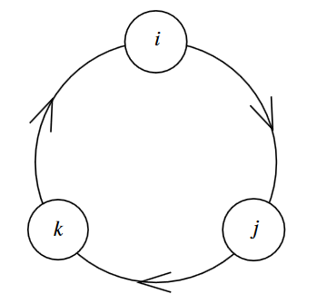
-
for all
-
for a cyclic permutation of then
(graphics grabbed from Baez 02)
Definition
The octonions is the nonassociative algebra over the real numbers which is generated from seven generators subject to the relations
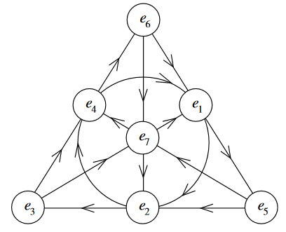
-
for all
-
for an edge or circle in the diagram shown (a labeled version of the Fano plane) then
and all relations obtained by cyclic permutation of the indices in these equations.
(graphics grabbed from Baez 02)
One defines the following operations on these real algebras:
Definition
(conjugation, real part, imaginary part and absolute value)
For , let
be the antihomomorphism of real algebras
given on the generators of def. , def. and def. by
This operation makes into a star algebra. For the complex numbers this is called complex conjugation, and in general we call it conjugation.
Let then
be the function
(“real part”) and
be the function
(“imaginary part”).
It follows that for all then the product of a with its conjugate is in the real center of
and we write the square root of this expression as
called the norm or absolute value function
This norm operation clearly satisfies the following properties (for all )
-
;
-
;
and hence makes a normed algebra.
Since is a division algebra, these relations immediately imply that each is a division algebra, in that
Hence the conjugation operation makes a real normed division algebra.
Remark
(sequence of inclusions of real normed division algebras)
Suitably embedding the sets of generators in def. , def. and def. into each other yields sequences of real star-algebra inclusions
For example for the first two inclusions we may send each generator to the generator of the same name, and for the last inclusion me may choose
Proposition
(Hurwitz theorem: , , and are the normed real division algebras)
The four algebras of real numbers , complex numbers , quaternions and octonions from def. , def. and def. respectively, which are real normed division algebras via def. , are, up to isomorphism, the only real normed division algebras that exist.
Remark
(Cayley-Dickson construction and sedenions)
While prop. says that the sequence from remark
is maximal in the category of real normed non-associative division algebras, there is a pattern that does continue if one disregards the division algebra property. Namely each step in this sequence is given by a construction called forming the Cayley-Dickson double algebra. This continues to an unbounded sequence of real nonassociative star-algebras
where the next algebra is called the sedenions.
What actually matters for the following relation of the real normed division algebras to real spin representations is that they are also alternative algebras:
Definition
Given any non-associative algebra , then the trilinear map
given on any elements by
is called the associator (in analogy with the commutator ).
If the associator is completely antisymmetric (in that for any permutation of three elements then for the signature of the permutation) then is called an alternative algebra.
If the characteristic of the ground field is different from 2, then alternativity is readily seen to be equivalent to the conditions that for all then
We record some basic properties of associators in alternative star-algebras that we need below:
Proposition
(properties of alternative star algebras)
Let be an alternative algebra (def. ) which is also a star algebra. Then (using def. ):
-
the associator vanishes when at least one argument is real
-
the associator changes sign when one of its arguments is conjugated
-
the associator vanishes when one of its arguments is the conjugate of another
-
the associator is purely imaginary
Proof
That the associator vanishes as soon as one argument is real is just the linearity of an algebra product over the ground ring.
Hence in fact
This implies the second statement by linearity. And so follows the third statement by skew-symmetry:
The fourth statement finally follows by this computation:
Here the first equation follows by inspection and using that , the second follows from the first statement above, and the third is the anti-symmetry of the associator.
It is immediate to check that:
Proposition
(, , and are real alternative algebras)
The real algebras of real numbers, complex numbers, def. ,quaternions def. and octonions def. are alternative algebras (def. ).
Proof
Since the real numbers, complex numbers and quaternions are associative algebras, their associator vanishes identically. It only remains to see that the associator of the octonions is skew-symmetric. By linearity it is sufficient to check this on generators. So let be a circle or a cyclic permutation of an edge in the Fano plane. Then by definition of the octonion multiplication we have
and similarly
The analog of the Hurwitz theorem (prop. ) is now this:
Proposition
(, , and are precisely the alternative real division algebras)
The only division algebras over the real numbers which are also alternative algebras (def. ) are the real numbers themselves, the complex numbers, the quaternions and the octonions from prop. .
This is due to (Zorn 30).
For the following, the key point of alternative algebras is this equivalent characterization:
Proposition
(alternative algebra detected on subalgebras spanned by any two elements)
A nonassociative algebra is alternative, def. , precisely if the subalgebra generated by any two elements is an associative algebra.
This is due to Emil Artin, see for instance (Schafer 95, p. 18).
Proposition is what allows to carry over a minimum of linear algebra also to the octonions such as to yield a representation of the Clifford algebra on . This happens in the proof of prop. below.
So we will be looking at a fragment of linear algebra over these four normed division algebras. To that end, fix the following notation and terminology:
Definition
(hermitian matrices with values in real normed division algebras)
Let be one of the four real normed division algebras from prop. , hence equivalently one of the four real alternative division algebras from prop. .
Say that an matrix with coefficients in
is a hermitian matrix if the transpose matrix equals the componentwise conjugated matrix (def. ):
Hence with the notation
we have that is a hermitian matrix precisely if
We write for the real vector space of hermitian matrices.
Definition
(trace reversal)
Let be a hermitian matrix as in def. . Its trace reversal is the result of subtracting its trace times the identity matrix:
Minkowski spacetime in dimensions 3,4,6 and 10
We now discover Minkowski spacetime of dimension 3,4,6 and 10, in terms of the real normed division algebras from prop. , equivalently the real alternative division algebras from prop. : this is prop./def. and def. below.
Proposition/Definition
(Minkowski spacetime as real vector space of hermitian matrices in real normed division algebras)
Let be one of the four real normed division algebras from prop. , hence one of the four real alternative division algebras from prop. .
Then the real vector space of hermitian matrices over (def. ) equipped with the inner product whose quadratic form is the negative of the determinant operation on matrices is Minkowski spacetime:
hence
-
for ;
-
for ;
-
for ;
-
for .
Here we think of the vector space on the left as with
equipped with the canonical coordinates labeled .
As a linear map the identification is given by
This means that the quadratic form is given on an element by
By the polarization identity the quadratic form induces a bilinear form
given by
This is called the Minkowski metric.
Finally, under the above identification the operation of trace reversal from def. corresponds to time reversal in that
Proof
We need to check that under the given identification, the Minkowski norm-square is indeed given by minus the determinant on the corresponding hermitian matrices. This follows from the nature of the conjugation operation from def. :
Remark
(physical units of length)
As the term “metric” suggests, in application to physics, the Minkowski metric in prop./def. is regarded as a measure of length: for a tangent vector at a point in Minkowski spacetime, interpreted as a displacement from event to event , then
-
if then
is interpreted as a measure for the spatial distance between and ;
-
if then
is interpreted as a measure for the time distance between and .
But for this to make physical sense, an operational prescription needs to be specified that tells the experimentor how the real number is to be translated into an physical distance between actual events in the observable universe.
Such an operational prescription is called a physical unit of length. For example “centimeter” is a physical unit of length, another one is “femtometer” .
The combined information of a real number and a physical unit of length such as meter, jointly written
is a prescription for finding actual distance in the observable universe. Alternatively
is another prescription, that translates the same real number into another physical distance.
But of course they are related, since physical units form a torsor over the group of non-negative real numbers, meaning that any two are related by a unique rescaling. For example
with .
This means that once any one prescription of turning real numbers into spacetime distances is specified, then any other such prescription is obtained from this by rescaling these real numbers. For example
The point to notice here is that, via the last line, we may think of this as rescaling the metric from to .
In quantum field theory physical units of length are typically expressed in terms of a physical unit of “action”, called “Planck's constant” , via the combination of units called the Compton wavelength
parameterized, in turn, by a physical unit of mass . For the mass of the electron, the Compton wavelength is
Another physical unit of length parameterized by a mass is the Schwarzschild radius , where is the gravitational constant. Solving the equation
for yields the Planck mass
The corresponding Compton wavelength is given by the Planck length
Definition
(Minkowski spacetime as a pseudo-Riemannian Cartesian space)
Prop./def. introduces Minkowski spacetime for as a a vector space equipped with a norm . The genuine spacetime corresponding to this is this vector space regaded as a Cartesian space, i.e. with smooth functions (instead of just linear maps) to it and from it (def. ). This still carries one copy of over each point , as its tangent space (example )
and the Cartesian space equipped with the Lorentzian inner product from prop./def. on each tangent space (a “pseudo-Riemannian Cartesian space”) is Minkowski spacetime as such.
We write
for the canonical volume form on Minkowski spacetime.
We use the Einstein summation convention: Expressions with repeated indices indicate summation over the range of indices.
For example a differential 1-form on Minkowski spacetime may be expanded as
Moreover we use square brackets around indices to indicate skew-symmetrization. For example a differential 2-form on Minkowski spacetime may be expanded as
The identification of Minkowski spacetime (def. ) in the exceptional dimensions with the generalized Pauli matrices (prop./def. ) has some immediate useful implications:
Proposition
(Minkowski metric in terms of trace reversal)
In terms of the trace reversal operation from def. , the determinant operation on hermitian matrices (def. ) has the following alternative expression
and the Minkowski inner product from prop. has the alternative expression
Proposition
(special linear group acts by linear isometries on Minkowski spacetime )
For one of the four real normed division algebras (prop. ) the special linear group acts on Minkowski spacetime in dimension (def. ) by linear isometries given under the identification with the Pauli matrices in prop./def. by conjugation:
Proof
For this is immediate from matrix calculus, but we spell it out now. While the argument does not directly apply to the case of the octonions, one can check that it still goes through, too.
First we need to see that the action is well defined. This follows from the associativity of matrix multiplication and the fact that forming conjugate transpose matrices is an antihomomorphism: . In particular this implies that the action indeed sends hermitian matrices to hermitian matrices:
By prop./def. such an action is an isometry precisely if it preserves the determinant. This follows from the multiplicative property of determinants: and their compativility with conjugate transposition: , and finally by the assumption that is an element of the special linear group, hence that its determinant is :
In fact the special linear groups of linear isometries in prop. are the spin groups (def. below) in these dimensions.
exceptional spinors and real normed division algebras
This we explain now.
Lorentz group and spin group
Definition
For , write
for the subgroup of the general linear group on those linear maps which preserve this bilinear form on Minkowski spacetime (def ), in that
This is the Lorentz group in dimension .
The elements in the Lorentz group in the image of the special orthogonal group are rotations in space. The further elements in the special Lorentz group , which mathematically are “hyperbolic rotations” in a space-time plane, are called boosts in physics.
One distinguishes the following further subgroups of the Lorentz group :
-
is the subgroup of elements which have determinant +1 (as elements of the general linear group);
-
the proper orthochronous (or restricted) Lorentz group
is the further subgroup of elements which preserve the time orientation of vectors in that .
Proposition
(connected component of Lorentz group)
As a smooth manifold, the Lorentz group (def. ) has four connected components. The connected component of the identity is the proper orthochronous Lorentz group (def. ). The other three components are
-
,
where, as matrices,
is the operation of point reflection at the origin in space, where
is the operation of reflection in time and hence where
is point reflection in spacetime.
The following concept of the Clifford algebra (def. ) of Minkowski spacetime encodes the structure of the inner product space in terms of algebraic operation (“geometric algebra”), such that the action of the Lorentz group becomes represented by a conjugation action (example below). In particular this means that every element of the proper orthochronous Lorentz group may be “split in half” to yield a double cover: the spin group (def. below).
Definition
For , we write
for the -graded associative algebra over which is generated from generators in odd degree (“Clifford generators”), subject to the relation
where is the inner product of Minkowski spacetime as in def. .
These relations say equivalently that
We write
for the antisymmetrized product of Clifford generators. In particular, if all the are pairwise distinct, then this is simply the plain product of generators
Finally, write
for the algebra anti-automorphism given by
Remark
(vectors inside Clifford algebra)
By construction, the vector space of linear combinations of the generators in a Clifford algebra (def. ) is canonically identified with Minkowski spacetime (def. )
via
hence via
such that the defining quadratic form on is identified with the anti-commutator in the Clifford algebra
where on the right we are, in turn, identifying with the linear span of the unit in .
The key point of the Clifford algebra (def. ) is that it realizes spacetime reflections, rotations and boosts via conjugation actions:
Example
(Clifford conjugation)
For and the Minkowski spacetime of def. , let be any vector, regarded as an element via remark .
Then
- the conjugation action of a single Clifford generator on sends to its
reflection at the hyperplane ;
-
sends to the result of rotating it in the -plane through an angle .
Proof
This is immediate by inspection:
For the first statement, observe that conjugating the Clifford generator with yields up to a sign, depending on whether or not:
Therefore for then is the result of multiplying the -component of by .
For the second statement, observe that
This is the canonical action of the Lorentzian special orthogonal Lie algebra . Hence
is the rotation action as claimed.
Remark
Since the reflections, rotations and boosts in example are given by conjugation actions, there is a crucial ambiguity in the Clifford elements that induce them:
-
the conjugation action by coincides precisely with the conjugation action by ;
-
the conjugation action by coincides precisely with the conjugation action by .
Definition
For , the spin group is the group of even graded elements of the Clifford algebra (def. ) which are unitary with respect to the conjugation operation from def. :
Proposition
The function
from the spin group (def. ) to the general linear group in -dimensions given by sending to the conjugation action
(via the identification of Minkowski spacetime as the subspace of the Clifford algebra containing the linear combinations of the generators, according to remark )
is
-
a group homomorphism onto the proper orthochronous Lorentz group (def. ):
-
exhibiting a -central extension.
Proof
That the function is a group homomorphism into the general linear group, hence that it acts by linear transformations on the generators follows by using that it clearly lands in automorphisms of the Clifford algebra.
That the function lands in the Lorentz group follows from remark :
That it moreover lands in the proper Lorentz group follows from observing (example ) that every reflection is given by the conjugation action by a linear combination of generators, which are excluded from the group (as that is defined to be in the even subalgebra).
To see that the homomorphism is surjective, use that all elements of are products of rotations in hyperplanes. If a hyperplane is spanned by the bivector , then such a rotation is given, via example by the conjugation action by
for some , hence is in the image.
That the kernel is is clear from the fact that the only even Clifford elements which commute with all vectors are the multiples of the identity. For these and hence the condition is equivalent to . It is clear that these two elements are in the center of . This kernel reflects the ambiguity from remark .
Spinors in dimensions 3, 4, 6 and 10
We now discuss how real spin representations (def. ) in spacetime dimensions 3,4, 6 and 10 are naturally induced from linear algebra over the four real alternative division algebras (prop. ).
Definition
(Clifford algebra via normed division algebra)
Let be one of the four real normed division algebras from prop. , hence one of the four real alternative division algebras from prop. .
Define a real linear map
from (the real vector space underlying) Minkowski spacetime to real linear maps on
Here on the right we are using the isomorphism from prop. for identifying a spacetime vector with a -matrix, and we are using the trace reversal from def. .
Remark
(Clifford multiplication via octonion-valued matrices)
Each operation of in def. is clearly a linear map, even for being the non-associative octonions. The only point to beware of is that for the octonions, then the composition of two such linear maps is not in general given by the usual matrix product.
Proposition
(real spin representations via normed division algebras)
The map in def. gives a representation of the Clifford algebra (this def.), i.e of
-
for ;
-
for ;
-
for ;
-
for .
Hence this Clifford representation induces representations of the spin group on the real vector spaces
and hence on
Proof
We need to check that the Clifford relation
is satisfied (where we used (11) and (8)). Now by definition, for any then
where on the right we have in each component ordinary matrix product expressions.
Now observe that both expressions on the right are sums of triple products that involve either one real factor or two factors that are conjugate to each other:
Since the associators of triple products that involve a real factor and those involving both an element and its conjugate vanish by prop. (hence ultimately by Artin’s theorem, prop. ). In conclusion all associators involved vanish, so that we may rebracket to obtain
Proposition
Let be one of the four real normed division algebras and the corresponding spin representation from prop. .
Then there are bilinear maps from two spinors (according to prop. ) to the real numbers
as well as to
given, respectively, by forming the real part (def. ) of the canonical -inner product
and by forming the product of a column vector with a row vector to produce a matrix, possibly up to trace reversal (def. ) under the identification from prop. :
and
For the -component of this map is
These pairings have the following properties
-
both are -equivalent;
-
the pairing is symmetric:
(12)
(Baez-Huerta 09, prop. 8, prop. 9).
Remark
(two-component spinor notation)
In the physics/QFT literature the expressions for spin representations given by prop. are traditionally written in two-component spinor notation as follows:
-
An element of is denoted and called a left handed spinor;
-
an element of is denoted and called a right handed spinor;
-
an element of is denoted
(13)and called a Dirac spinor;
and the Clifford action of prop. corresponds to the generalized “Pauli matrices”:
-
a hermitian matrix as in prop regarded as a linear map via def. is denoted
-
the negative of the trace-reversal (def. ) of such a hermitian matrix, regarded as a linear map , is denoted
-
the bilinear spinor-to-vector pairing from prop. is written as the matrix multiplication
where the Dirac conjugate on the left is given on by
(14)hence, with (13):
(15)
Finally, it is common to abbreviate contractions with the Clifford algebra generators by a slash, as in
or
This is called the Feynman slash notation.
(e.g. Dermisek I-8, Dermisek I-9)
Below we spell out the example of the Lagrangian field theory of the Dirac field in detail (example ). For discussion of massive chiral spinor fields one also needs the following, here we just mention this for completeness:
Proposition
(chiral spinor mass pairing)
In dimension 2+1 and 3+1, there exists a non-trivial skew-symmetric pairing
which may be normalized such that in the two-component spinor basis of remark we have
Proof
Take the non-vanishing components of to be
and
With this equation (17) is checked explicitly. It is clear that thus defined is skew symmetric as long as the component algebra is commutative, which is the case for being or .
Causal structure
We need to consider the following concepts and constructions related to the causal structure of Minkowski spacetime (def. ).
Definition
(spacelike, timelike, lightlike directions; past and future)
Given two points in Minkowski spacetime (def. ), write
for their difference, using the vector space structure underlying Minkowski spacetime.
Recall the Minkowski inner product on , given by prop./def. . Then via remark we say that the difference vector is
Definition
For a point in spacetime (an event), we write
for the subsets of events that are in the timelike future or in the timelike past of , respectively (def. ) called the open future cone and open past cone, respectively, and
for the subsets of events that are in the timelike or lightlike future or past, respectivel, called the closed future cone and closed past cone, respectively.
The union
of the closed future cone and past cone is called the full causal cone of the event . Its boundary is the light cone.
More generally for a subset of events we write
for the union of the future/past closed cones of all events in the subset.
Definition
(compactly sourced causal support)
Consider a vector bundle (def. ) over Minkowski spacetime (def. ).
Write for the spaces of smooth sections (def. ), and write
for the subsets on those smooth sections whose support is
-
() inside a compact subset,
-
() inside the closed future cone/closed past cone, respectively, of a compact subset,
-
() inside the closed causal cone of a compact subset, which equivalently means that the intersection with every (spacelike) Cauchy surface is compact (Sanders 13, theorem 2.2),
-
() inside the past of a Cauchy surface (Sanders 13, def. 3.2),
-
() inside the future of a Cauchy surface (Sanders 13, def. 3.2),
-
() inside the future of one Cauchy surface and the past of another (Sanders 13, def. 3.2).
(Bär 14, section 1, Khavkine 14, def. 2.1)
Definition
Consider the relation on the set of subsets of spacetime which says a subset is not prior to a subset , denoted , if does not intersect the causal past of (def. ), or equivalently that does not intersect the causal future of :
(Beware that this is just a relation, not an ordering, since it is not relation.)
If and we say that the two subsets are spacelike separated and write
Definition
(causal complement and causal closure of subset of spacetime)
For a subset of spacetime, its causal complement is the complement of the causal cone:
The causal complement of the causal complement is called the causal closure. If
then the subset is called a causally closed subset.
Given a spacetime , we write
for the partially ordered set of causally closed subsets, partially ordered by inclusion .
Definition
For a causally closed subset of spacetime (def. ) say that an adiabatic switching function or infrared cutoff function for is a smooth function of compact support (a bump function) whose restriction to some neighbourhood of is the constant function with value :
Often we consider the vector space space spanned by a formal variable (the coupling constant) under multiplication with smooth functions, and consider as adiabatic switching functions the corresponding images in this space,
which are thus bump functions constant over a neighbourhood of not on 1 but on the formal parameter :
In this sense we may think of the adiabatic switching as being the spacetime-depependent coupling “constant”.
The following lemma will be key in the derivation (proof of prop. below) of the causal locality of algebra of quantum observables in perturbative quantum field theory:
Lemma
(causal partition)
Let be a causally closed subset (def. ) and let be a compactly supported smooth function which vanishes on a neighbourhood , i.e. .
Then there exists a causal partition of in that there exist compactly supported smooth functions such that
-
they sum up to :
-
their support satisfies the following causal ordering (def. )
Proof idea
By assumption has a Cauchy surface. This may be extended to a Cauchy surface of , such that this is one leaf of a foliation of by Cauchy surfaces, given by a diffeomorphism with the original at zero. There exists then such that the restriction of to the interval is in the causal complement of the given region (def. ):
Let then be any smooth function with
-
.
Then
are smooth functions as required.
This concludes our discussion of spin and spacetime. In the next chapter we consider the concept of fields on spacetime.
Fields
In this chapter we discuss these topics:
A field history on a given spacetime (a history of spatial field configurations, see remark below) is a quantity assigned to each point of spacetime (each event), such that this assignment varies smoothly with spacetime points. For instance an electromagnetic field history (example below) is at each point of spacetime a collection of vectors that encode the direction in which a charged particle passing through that point would feel a force (the “Lorentz force”, see example below).
This is readily formalized (def. below): If denotes the smooth manifold of “values” that the given kind of field may take at any spacetime point, then a field history is modeled as a smooth function from spacetime to this space of values:
It will be useful to unify spacetime and the space of field values (the field fiber) into a single manifold, the Cartesian product
and to think of this equipped with the projection map onto the first factor as a fiber bundle of spaces of field values over spacetime
This is then called the field bundle, which specifies the kind of values that the given field species may take at any point of spacetime. Since the space of field values is the fiber of this fiber bundle (def. ), it is sometimes also called the field fiber. (See also at fiber bundles in physics.)
Given a field bundle , then a field history is a section of that bundle (def. ). The discussion of field theory concerns the space of all possible field histories, hence the space of sections of the field bundle (example below). This is a very “large” generalized smooth space, called a diffeological space (def. below).
Or rather, in the presence of fermion fields such as the Dirac field (example below), the Pauli exclusion principle demands that the field bundle is a super-manifold, and that the fermionic space of field histories (example below) is a super-geometric generalized smooth space: a super smooth set (def. below).
This smooth structure on the space of field histories will be crucial when we discuss observables of a field theory below, because these are smooth functions on the space of field histories. In particular it is this smooth structure which allows to derive that linear observables of a free field theory are given by distributions (prop. ) below. Among these are the point evaluation observables (delta distributions) which are traditionally denoted by the same symbol as the field histories themselves.
Hence there are these aspects of the concept of “field” in physics, which are closely related, but crucially different:
aspects of the concept of fields
| aspect | term | type | description | def. |
|---|---|---|---|---|
| field component | , | coordinate function on jet bundle of field bundle | def. , def. | |
| field history | , | jet prolongation of section of field bundle | def. , def. | |
| field observable | , | derivatives of delta-functional on space of sections | def. , example | |
| averaging of field observable | observable-valued distribution | def. | ||
| algebra of quantum observables | non-commutative algebra structure on field observables | def. , def. |
Definition
(fields and field histories)
Given a spacetime , then a type of fields on is a smooth fiber bundle (def. )
called the field bundle,
Given a type of fields on this way, then a field history of that type on is a term of that type, hence is a smooth section (def. ) of this bundle, namely a smooth function of the form
such that composed with the projection map it is the identity function, i.e. such that
The set of such sections/field histories is to be denoted
Remark
(field histories are histories of spatial field configurations)
Given a section of the field bundle (def. ) and given a spacelike (def. ) submanifold (def. ) of spacetime in codimension 1, then the restriction of to may be thought of as a field configuration in space. As different spatial slices are chosen, one obtains such field configurations at different times. It is in this sense that the entirety of a section is a history of field configurations, hence a field history (def ).
Remark
(possible field histories)
After we give the set of field histories (18) differential geometric structure, below in example and example , we call it the space of field histories. This should be read as space of possible field histories; containing all field histories that qualify as being of the type specified by the field bundle .
After we obtain equations of motion below in def. , these serve as the “laws of nature” that field histories should obey, and they define the subspace of those field histories that do solve the equations of motion; this will be denoted
and called the on-shell space of field histories (41).
For the time being, not to get distracted from the basic idea of quantum field theory, we will focus on the following simple special case of field bundles:
Example
(trivial vector bundle as a field bundle)
In applications the field fiber is often a finite dimensional vector space. In this case the trivial field bundle with fiber is of course a trivial vector bundle (def. ).
Choosing any linear basis of the field fiber, then over Minkowski spacetime (def. ) we have canonical coordinates on the total space of the field bundle
where the index ranges from to , while the index ranges from 1 to .
If this trivial vector bundle is regarded as a field bundle according to def. , then a field history is equivalently an -tuple of real-valued smooth functions on spacetime:
Example
(field bundle for real scalar field)
If is a spacetime and if the field fiber
is simply the real line, then the corresponding trivial field bundle (def. )
is the trivial real line bundle (a special case of example ) and the corresponding field type (def. ) is called the real scalar field on . A configuration of this field is simply a smooth function on with values in the real numbers:
Example
(field bundle for electromagnetic field)
On Minkowski spacetime (def. ), let the field bundle (def. ) be given by the cotangent bundle
This is a trivial vector bundle (example ) with canonical field coordinates .
A section of this bundle, hence a field history, is a differential 1-form
on spacetime (def. ). Interpreted as a field history of the electromagnetic field on , this is often called the vector potential. Then the de Rham differential (def. ) of the vector potential is a differential 2-form
known as the Faraday tensor. In the canonical coordinate basis 2-forms this may be expanded as
Here are called the components of the electric field, while are called the components of the magnetic field.
Example
(field bundle for Yang-Mills field over Minkowski spacetime)
Let be a Lie algebra of finite dimension with linear basis , in terms of which the Lie bracket is given by
Over Minkowski spacetime (def. ), consider then the field bundle which is the cotangent bundle tensored with the Lie algebra
This is the trivial vector bundle (example ) with induced field coordinates
A section of this bundle is a Lie algebra-valued differential 1-form
with components
This is called a field history for Yang-Mills gauge theory (at least if is a semisimple Lie algebra, see example below).
For is the line Lie algebra, this reduces to the case of the electromagnetic field (example ).
For this is a field history for the gauge field of the strong nuclear force in quantum chromodynamics.
For readers familiar with the concepts of principal bundles and connections on a bundle we include the following example which generalizes the Yang-Mills field over Minkowski spacetime from example to the situation over general spacetimes.
Example
(general Yang-Mills field in fixed topological sector)
Let be any spacetime manifold and let be a compact Lie group with Lie algebra denoted . Let be a -principal bundle and a chosen connection on it, to be called the background -Yang-Mills field.
Then the field bundle (def. ) for -Yang-Mills theory in the topological sector is the tensor product of vector bundles
of the adjoint bundle of and the cotangent bundle of .
With the choice of , every (other) connection on uniquely decomposes as
where
is a section of the above field bundle, hence a Yang-Mills field history.
The electromagnetic field (def. ) and the Yang-Mills field (def. , def. ) with differential 1-forms as field histories are the basic examples of gauge fields (we consider this in more detail below in Gauge symmetries). There are also higher gauge fields with differential n-forms as field histories:
Example
(field bundle for B-field)
On Minkowski spacetime (def. ), let the field bundle (def. ) be given by the skew-symmetrized tensor product of vector bundles of the cotangent bundle with itself
This is a trivial vector bundle (example ) with canonical field coordinates subject to
A section of this bundle, hence a field history, is a differential 2-form (def. )
on spacetime.
Given any field bundle, we will eventually need to regard the set of all field histories as a “smooth set” itself, a smooth space of sections, to which constructions of differential geometry apply (such as for the discussion of observables and states below ). Notably we need to be talking about differential forms on .
However, a space of sections does not in general carry the structure of a smooth manifold; and it carries the correct smooth structure of an infinite dimensional manifold only if is a compact space (see at manifold structure of mapping spaces). Even if it does carry infinite dimensional manifold structure, inspection shows that this is more structure than actually needed for the discussion of field theory. Namely it turns out below that all we need to know is what counts as a smooth family of sections/field histories, hence which functions of sets
from any Cartesian space (def. ) into count as smooth functions, subject to some basic consistency condition on this choice.
This structure on is called the structure of a diffeological space:
Definition
A diffeological space is
-
for each a choice of subset
of the set of functions from the underlying set of to , to be called the smooth functions or plots from to ;
-
for each smooth function between Cartesian spaces (def. ) a choice of function
to be thought of as the precomposition operation
such that
-
(constant functions are smooth)
-
-
If is the identity function on , then is the identity function on the set of plots ;
-
If are two composable smooth functions between Cartesian spaces (def. ), then pullback of plots along them consecutively equals the pullback along the composition:
i.e.
-
-
(gluing)
If is a differentiably good open cover of a Cartesian space (def. ) then the function which restricts -plots of to a set of -plots
is a bijection onto the set of those tuples of plots, which are “matching families” in that they agree on intersections:
Finally, given and two diffeological spaces, then a smooth function between them
is
-
a function of the underlying sets
such that
-
for a plot of , then the composition is a plot of :
(Stated more abstractly, this says simply that diffeological spaces are the concrete sheaves on the site of Cartesian spaces from def. .)
For more background on diffeological spaces see also geometry of physics – smooth sets.
Example
(Cartesian spaces are diffeological spaces)
Let be a Cartesian space (def. ) Then it becomes a diffeological space (def. ) by declaring its plots to the ordinary smooth functions .
Under this identification, a function between the underlying sets of two Cartesian spaces is a smooth function in the ordinary sense precisely if it is a smooth function in the sense of diffeological spaces.
Stated more abstractly, this statement is an example of the Yoneda embedding over a subcanonical site.
More generally, the same construction makes every smooth manifold a smooth set.
Example
(diffeological space of field histories)
Let be a smooth field bundle (def. ). Then the set of field histories/sections (def. ) becomes a diffeological space (def. )
by declaring that a smooth family of field histories, parameterized over any Cartesian space is a smooth function out of the Cartesian product manifold of with
such that for each we have , i.e.
The following example is included only for readers who wonder how infinite-dimensional manifolds fit in. Since we will never actually use infinite-dimensional manifold-structure, this example is may be ignored.
Example
(Fréchet manifolds are diffeological spaces)
Consider the particular type of infinite-dimensional manifolds called Fréchet manifolds. Since ordinary smooth manifolds are an example, for a Fréchet manifold there is a concept of smooth functions . Hence we may give the structure of a diffeological space (def. ) by declaring the plots over to be these smooth functions , with the evident postcomposition action.
It turns out that then that for and two Fréchet manifolds, there is a natural bijection between the smooth functions between them regarded as Fréchet manifolds and [regarded as . Hence it does not matter which of the two perspectives we take (unless of course a more general than a enters the picture, at which point the second definition generalizes, whereas the first does not).]
Stated more abstractly, this means that Fréchet manifolds form a full subcategory of that of diffeological spaces (this prop.):
If is a compact smooth manifold and is a trivial fiber bundle with fiber a smooth manifold, then the set of sections carries a standard structure of a Fréchet manifold (see at manifold structure of mapping spaces). Under the above inclusion of Fréchet manifolds into diffeological spaces, this smooth structure agrees with that from example (see this prop.)
Once the step from smooth manifolds to diffeological spaces (def. ) is made, characterizing the smooth structure of the space entirely by how we may probe it by mapping smooth Cartesian spaces into it, it becomes clear that the underlying set of a diffeological space is not actually crucial to support the concept: The space is already entirely defined structurally by the system of smooth plots it has, and the underlying set is recovered from these as the set of plots from the point .
This is crucial for field theory: the spaces of field histories of fermionic fields (def. below) such as the Dirac field (example below) do not have underlying sets of points the way diffeological spaces have. Informally, the reason is that a point is a bosonic object, while and the nature of fermionic fields is the opposite of bosonic.
But we may just as well drop the mentioning of the underlying set in the definition of generalized smooth spaces. By simply stripping this requirement off of def. we obtain the following more general and more useful definition (still “bosonic”, though, the supergeometric version is def. below):
Definition
A smooth set is
-
for each a choice of set
to be called the set of smooth functions or plots from to ;
-
for each smooth function between Cartesian spaces a choice of function
to be thought of as the precomposition operation
such that
-
-
If is the identity function on , then is the identity function on the set of plots .
-
If are two composable smooth functions between Cartesian spaces, then consecutive pullback of plots along them equals the pullback along the composition:
i.e.
-
-
(gluing)
If is a differentiably good open cover of a Cartesian space (def. ) then the function which restricts -plots of to a set of -plots
is a bijection onto the set of those tuples of plots, which are “matching families” in that they agree on intersections:
Finally, given and two smooth sets, then a smooth function between them
is
-
for each a function
such that
-
for each smooth function between Cartesian spaces we have
Stated more abstractly, this simply says that smooth sets are the sheaves on the site of Cartesian spaces from def. .
Basing differential geometry on smooth sets is an instance of the general approach to geometry called functorial geometry or topos theory. For more background on this see at geometry of physics – smooth sets.
First we verify that the concept of smooth sets is a consistent generalization:
Example
(diffeological spaces are smooth sets)
Every diffeological space (def. ) is a smooth set (def. ) simply by forgetting its underlying set of points and remembering only its sets of plot.
In particular therefore each Cartesian space is canonically a smooth set by example .
Moreover, given any two diffeological spaces, then the morphisms between them, regarded as diffeological spaces, are the same as the morphisms as smooth sets.
Stated more abstractly, this means that we have full subcategory inclusions
Recall, for the next proposition , that in the definition of a smooth set the sets are abstract sets which are to be thought of as would-be smooth functions “”. Inside def. this only makes sense in quotation marks, since inside that definition the smooth set is only being defined, so that inside that definition there is not yet an actual concept of smooth functions of the form “”.
But now that the definition of smooth sets and of morphisms between them has been stated, and seeing that Cartesian space are examples of smooth sets, by example , there is now an actual concept of smooth functions , namely as smooth sets. For the concept of smooth sets to be consistent, it ought to be true that this a posteriori concept of smooth functions from Cartesian spaces to smooth sets coincides wth the a priori concept, hence that we “may remove the quotation marks” in the above. The following proposition says that this is indeed the case:
Proposition
(plots of a smooth set really are the smooth functions into the smooth set)
Let be a smooth set (def. ). For , there is a natural function
from the set of homomorphisms of smooth sets from (regarded as a smooth set via example ) to , to the set of plots of over , given by evaluating on the identity plot .
This function is a bijection.
This says that the plots of , which initially bootstrap into being as declaring the would-be smooth functions into , end up being the actual smooth functions into .
Proof
This elementary but profound fact is called the Yoneda lemma, here in its incarnation over the site of Cartesian spaces (def. ).
A key class of examples of smooth sets (def. ) that are not diffeological spaces (def. ) are universal smooth moduli spaces of differential forms:
Example
(universal smooth moduli spaces of differential forms)
For there is a smooth set (def. )
defined as follows:
-
for the set of plots from to is the set of smooth differential k-forms on (def. )
-
for a smooth function (def. ) the operation of pullback of plots along is just the pullback of differential forms from prop.
That this is functorial is just the standard fact (7) from prop. .
For the smooth set actually is a diffeological space, in fact under the identification of example this is just the real line:
But for we have that the set of plots on is a singleton
consisting just of the zero differential form. The only diffeological space with this property is itself. But is far from being that trivial: even though its would-be underlying set is a single point, for all it admits an infinite set of plots. Therefore the smooth sets for are not diffeological spaces.
That the smooth set indeed deserves to be addressed as the universal moduli space of differential k-forms follows from prop. : The universal moduli space of -forms ought to carry a universal differential -forms such that every differential -form on any arises as the pullback of differential forms of this universal one along some modulating morphism :
But with prop. this is precisely what the definition of the plots of says.
Similarly, all the usual operations on differential form now have their universal archetype on the universal moduli spaces of differential forms
In particular, for there is a canonical morphism of smooth sets of the form
defined over by the ordinary de Rham differential (def. )
That this satisfies the compatibility with precomposition of plots
is just the compatibility of pullback of differential forms with the de Rham differential of from prop. .
The upshot is that we now have a good definition of differential forms on any diffeological space and more generally on any smooth set:
Definition
(differential forms on smooth sets)
Let be a diffeological space (def. ) or more generally a smooth set (def. ) then a differential k-form on is equivalently a morphism of smooth sets
from to the universal smooth moduli space of differential froms from example .
Concretely, by unwinding the definitions of and of morphisms of smooth sets, this means that such a differential form is:
-
for each and each plot an ordinary differential form
such that
-
for each smooth function between Cartesian spaces the ordinary pullback of differential forms along is compatible with these choices, in that for every plot we have
i.e.
We write for the set of differential forms on the smooth set defined this way.
Moreover, given a differential k-form
on a smooth set this way, then its de Rham differential is given by the composite of morphisms of smooth sets with the universal de Rham differential from (23):
Explicitly this means simply that for a plot, then
The usual operations on ordinary differential forms directly generalize plot-wise to differential forms on diffeological spaces and more generally on smooth sets:
Definition
(exterior differential and exterior product on smooth sets)
Let be a diffeological space (def. ) or more generally a smooth set (def. ). Then
-
For a differential form on (def. ) its exterior differential
is defined on any plot as the ordinary exterior differential of the pullback of along that plot:
-
For and two differential forms on (def. ) then their exterior product
is the differential form defined on any plot as the ordinary exterior product of the pullback of th differential forms and to this plot:
Infinitesimal geometry
It is crucial in field theory that we consider field histories not only over all of spacetime, but also restricted to submanifolds of spacetime. Or rather, what is actually of interest are the restrictions of the field histories to the infinitesimal neighbourhoods (example below) of these submanifolds. This appears notably in the construction of phase spaces below. Moreover, fermion fields such as the Dirac field (example below) take values in graded infinitesimal spaces, called super spaces (discussed below). Therefore “infinitesimal geometry”, sometimes called formal geometry (as in “formal scheme”) or synthetic differential geometry or synthetic differential supergeometry, is a central aspect of field theory.
In order to mathematically grasp what infinitesimal neighbourhoods are, we appeal to the first magic algebraic property of differential geometry from prop. , which says that we may recognize smooth manifolds dually in terms of their commutative algebras of smooth functions on them
But since there are of course more algebras than arise this way from smooth manifolds, we may turn this around and try to regard any algebra as defining a would-be space, which would have as its algebra of functions.
For example an infinitesimally thickened point should be a space which is “so small” that every smooth function on it which vanishes at the origin takes values so tiny that some finite power of them is not just even more tiny, but actually vanishes:
Definition
(infinitesimally thickened Cartesian space)
An infinitesimally thickened point
is represented by a commutative algebra which as a real vector space is a direct sum
of the 1-dimensional space of multiples of 1 with a finite dimensional vector space that is a nilpotent ideal in that for each element there exists a natural number such that
More generally, an infinitesimally thickened Cartesian space
is represented by a commutative algebra
which is the tensor product of algebras of the algebra of smooth functions on an actual Cartesian space of some dimension (example ), with an algebra of functions of an infinitesimally thickened point, as above.
We say that a smooth function between two infinitesimally thickened Cartesian spaces
is by definition dually an -algebra homomorphism of the form
Example
(infinitesimal neighbourhoods in the real line )
Consider the quotient algebra of the formal power series algebra in a single parameter by the ideal generated by :
(This is sometimes called the algebra of dual numbers, for no good reason.) The underlying real vector space of this algebra is, as show, the direct sum of the multiples of 1 with the multiples of . A general element in this algebra is of the form
where are real numbers. The product in this algebra is given by “multiplying out” as usual, and discarding all terms proportional to :
We may think of an element as the truncation to first order of a Taylor series at the origin of a smooth function on the real line
where is the value of the function at the origin, and where is its first derivative at the origin.
Therefore this algebra behaves like the algebra of smooth function on an infinitesimal neighbourhood of which is so tiny that its elements become, upon squaring them, not just tinier, but actually zero:
This intuitive picture is now made precise by the concept of infinitesimally thickened points def. , if we simply set
and observe that there is the inclusion of infinitesimally thickened Cartesian spaces
which is dually given by the algebra homomorphism
which sends a smooth function to its value at zero plus times its derivative at zero. Observe that this is indeed a homomorphism of algebras due to the product law of differentiation, which says that
Hence we see that restricting a smooth function to the infinitesimal neighbourhood of a point is equivalent to restricting attention to its Taylor series to the given order at that point:
Similarly for each the algebra
may be thought of as the algebra of Taylor series at the origin of of smooth functions , where all terms of order higher than are discarded. The corresponding infinitesimally thickened point is often denoted
This is now the subobject of the real line
on those elements such that .
The following example shows that infinitesimal thickening is invisible for ordinary spaces when mapping out of these. In contrast example further below shows that the morphisms into an ordinary space out of an infinitesimal space are interesting: these are tangent vectors and their higher order infinitesimal analogs.
Example
(infinitesimal line has unique global point)
For any ordinary Cartesian space (def. ) and the order- infinitesimal neighbourhood of the origin in the real line from example , there is exactly only one possible morphism of infinitesimally thickened Cartesian spaces from to :
Proof
By definition such a morphism is dually an algebra homomorphism
from the higher order “algebra of dual numbers” to the algebra of smooth functions (example ).
Now this being an -algebra homomorphism, its action on the multiples of the identity is fixed:
All the remaining elements are proportional to , and hence are nilpotent. However, by the homomorphism property of an algebra homomorphism it follows that it must send nilpotent elements to nilpotent elements , because
But the only nilpotent element in is the zero element, and hence it follows that
Thus as above is uniquely fixed.
Example
(synthetic tangent vector fields)
Let be a Cartesian space (def. ), regarded as an infinitesimally thickened Cartesian space (def. ) and consider the first order infinitesimal line from example .
Then homomorphisms of infinitesimally thickened Cartesian spaces of the form
hence smoothly -parameterized collections of morphisms
which send the unique base point (example ) to , are in natural bijection with tangent vector fields (example ).
Proof
By definition, the morphisms in question are dually -algebra homomorphisms of the form
which are the identity modulo . Such a morphism has to take any function to
for some smooth function . The condition that this assignment makes an algebra homomorphism is equivalent to the statement that for all we have
Multiplying this out and using that , this is equivalent to
This in turn means equivalently that is a derivation.
With this the statement follows with the third magic algebraic property of smooth functions (prop. ): derivations of smooth functions are vector fields.
We need to consider infinitesimally thickened spaces more general than the thickenings of just Cartesian spaces in def. . But just as Cartesian spaces (def. ) serve as the local test geometries to induce the general concept of diffeological spaces and smooth sets (def. ), so using infinitesimally thickened Cartesian spaces as test geometries immediately induces the corresponding generalization of smooth sets with infinitesimals:
Definition
A formal smooth set is
-
for each infinitesimally thickened Cartesian space (def. ) a set
to be called the set of smooth functions or plots from to ;
-
for each smooth function between infinitesimally thickened Cartesian spaces a choice of function
to be thought of as the precomposition operation
such that
-
-
If is the identity function on , then is the identity function on the set of plots ;
-
If are two composable smooth functions between infinitesimally thickened Cartesian spaces, then pullback of plots along them consecutively equals the pullback along the composition:
i.e.
-
-
(gluing)
If is such that
in a differentiably good open cover (def. ) then the function which restricts -plots of to a set of -plots
is a bijection onto the set of those tuples of plots, which are “matching families” in that they agree on intersections:
i.e.
Finally, given and two formal smooth sets, then a smooth function between them
is
-
for each infinitesimally thickened Cartesian space (def. ) a function
such that
-
for each smooth function between infinitesimally thickened Cartesian spaces we have
i.e.
(Dubuc 79)
Basing infinitesimal geometry on formal smooth sets is an instance of the general approach to geometry called functorial geometry or topos theory. For more background on this see at geometry of physics – manifolds and orbifolds.
We have the evident generalization of example to smooth geometry with infinitesimals:
Example
(infinitesimally thickened Cartesian spaces are formal smooth sets)
For an infinitesimally thickened Cartesian space (def. ), it becomes a formal smooth set according to def. by taking its plots out of some to be the homomorphism of infinitesimally thickened Cartesian spaces:
(Stated more abstractly, this is an instance of the Yoneda embedding over a subcanonical site.)
Example
(smooth sets are formal smooth sets)
Let be a smooth set (def. ). Then becomes a formal smooth set (def. ) by declaring the set of plots over an infinitesimally thickened Cartesian space (def. ) to be equivalence classes of pairs
of a morphism of infinitesimally thickened Cartesian spaces and of a plot of , as shown, subject to the equivalence relation which identifies two such pairs if there exists a smooth function such that
Stated more abstractly this says that as a formal smooth set is the left Kan extension (see this example) of as a smooth set along the functor that includes Cartesian spaces (def. ) into infinitesimally thickened Cartesian spaces (def. ).
Definition
(reduction and infinitesimal shape)
For an infinitesimally thickened Cartesian space (def. ) we say that the underlying ordinary Cartesian space (def. ) is its reduction
There is the canonical inclusion morphism
which dually corresponds to the homomorphism of commutative algebras
which is the identity on all smooth functions and is zero on all elements in the nilpotent ideal of (as in example ).
Given any formal smooth set , we say that its infinitesimal shape or de Rham shape (also: de Rham stack) is the formal smooth set (def. ) defined to have as plots the reductions of the plots of , according to the above:
There is a canonical morphism of formal smooth set
which takes a plot
to the composition
regarded as a plot of .
Example
(mapping space out of an infinitesimally thickened Cartesian space)
Let be an infinitesimally thickened Cartesian space (def. ) and let be a formal smooth set (def. ). Then the mapping space
of smooth functions from to is the formal smooth set whose -plots are the morphisms of formal smooth sets from the Cartesian product of infinitesimally thickened Cartesian spaces to , hence the -plots of :
Example
Let be a Cartesian space (def. ) regarded as an infinitesimally thickened Cartesian space () and thus regarded as a formal smooth set (def. ) by example . Consider the infinitesimal line
from example . Then the mapping space (example ) is the total space of the tangent bundle (example ). Moreover, under restriction along the reduction , this is the full tangent bundle projection, in that there is a natural isomorphism of formal smooth sets of the form
In particular this implies immediately that smooth sections (def. ) of the tangent bundle
are equivalently morphisms of the form
which we had already identified with tangent vector fields (def. ) in example .
Proof
This follows by an analogous argument as in example , using the Hadamard lemma.
While in infinitesimally thickened Cartesian spaces (def. ) only infinitesimals to any finite order may exist, in formal smooth sets (def. ) we may find infinitesimals to any arbitrary finite order:
Example
Let be a formal smooth sets (def. ) a sub-formal smooth set. Then the infinitesimal neighbourhood to arbitrary infinitesimal order of in is the formal smooth set whose plots are those plots of
such that their reduction (def. )
factors through a plot of .
This allows to grasp the restriction of field histories to the infinitesimal neighbourhood of a submanifold of spacetime, which will be crucial for the discussion of phase spaces below.
Definition
(field histories on infinitesimal neighbourhood of submanifold of spacetime)
Let be a field bundle (def. ) and let be a submanifold of spacetime.
We write for its infinitesimal neighbourhood in (def. ).
Then the set of field histories restricted to , to be denoted
is the set of section of restricted to the infinitesimal neighbourhood (example ).
We close the discussion of infinitesimal differential geometry by explaining how we may recover the concept of smooth manifolds inside the more general formal smooth sets (def./prop. below). The key point is that the presence of infinitesimals in the theory allows an intrinsic definition of local diffeomorphisms/formally étale morphism (def. and example below). It is noteworthy that the only role this concept plays in the development of field theory below is that smooth manifolds admit triangulations by smooth singular simplices (def. ) so that the concept of fiber integration of differential forms is well defined over manifolds.
Definition
(local diffeomorphism of formal smooth sets)
Let be formal smooth sets (def. ). Then a morphism between them is called a local diffeomorphism or formally étale morphism, denoted
if if for each infinitesimally thickened Cartesian space (def. ) we have a natural identification between the -plots of with those -plots of whose reduction (def. ) comes from an -plot of , hence if we have a natural fiber product of sets of plots
i. e.
for all infinitesimally thickened Cartesian spaces .
Stated more abstractly, this means that the naturality square of the unit of the infinitesimal shape (def. ) is a pullback square
(Khavkine-Schreiber 17, def. 3.1)
Example
(local diffeomorphism between Cartesian spaces from the general definition)
For two ordinary Cartesian spaces (def. ), regarded as formal smooth sets by example then a morphism between them is a local diffeomorphism in the general sense of def. precisely if it is so in the ordinary sense of def. .
(Khavkine-Schreiber 17, prop. 3.2)
Definition/Proposition
A smooth manifold of dimension is
- a diffeological space (def. )
such that
-
there exists an indexed set of morphisms of formal smooth sets (def. ) from Cartesian spaces (def. ) (regarded as formal smooth sets via example , example and example ) into , (regarded as a formal smooth set via example and example ) such that
-
every point is in the image of at least one of the ;
-
every is a local diffeomorphism according to def. ;
-
-
the final topology induced by the set of plots of makes a paracompact Hausdorff space.
(Khavkine-Schreiber 17, example 3.4)
For more on smooth manifolds from the perspective of formal smooth sets see at geometry of physics – manifolds and orbifolds.
fermion fields and supergeometry
Field theories of interest crucially involve fermionic fields (def. below), such as the Dirac field (example below), which are subject to the “Pauli exclusion principle”, a key reason for the stability of matter. Mathematically this principle means that these fields have field bundles whose field fiber is not an ordinary manifold, but an odd-graded supermanifold (more on this in remark and remark below).
This “supergeometry” is an immediate generalization of the infinitesimal geometry above, where now the infinitesimal elements in the algebra of functions may be equipped with a grading: one speaks of superalgebra.
The “super”-terminology for something as down-to-earth as the mathematical principle behind the stability of matter may seem unfortunate. For better or worse, this terminology has become standard since the middle of the 20th century. But the concept that today is called supercommutative superalgebra was in fact first considered by Grassmann 1844 who got it right (“Ausdehnungslehre”) but apparently was too far ahead of his time and remained unappreciated.
Beware that considering supergeometry does not necessarily involve considering “supersymmetry”. Supergeometry is the geometry of fermion fields (def. below), and that all matter fields in the observable universe are fermionic has been experimentally established since the Stern-Gerlach experiment in 1922. Supersymmetry, on the other hand, is a hypothetical extension of spacetime-symmetry within the context of supergeometry. Here we do not discuss supersymmetry; for details see instead at geometry of physics – supersymmetry.
Definition
(supercommutative superalgebra)
A real -graded algebra or superalgebra is an associative algebra over the real numbers together with a direct sum decomposition of its underlying real vector space
such that the product in the algebra respects the multiplication in the cyclic group of order 2 :
This is called a supercommutative superalgebra if for all elements which are of homogeneous degree in that
we have
A homomorphism of superalgebras
is a homomorphism of associative algebras over the real numbers such that the -grading is respected in that
For more details on superalgebra see at geometry of physics – superalgebra.
Example
(basic examples of supercommutative superalgebras)
Basic examples of supercommutative superalgebras (def. ) include the following:
-
Every commutative algebra becomes a supercommutative superalgebra by declaring it to be all in even degree: .
-
For a finite dimensional real vector space, then the Grassmann algebra is a supercommutative superalgebra with and .
More explicitly, if is a Cartesian space with canonical dual coordinates then the Grassmann algebra is the real algebra which is generated from the regarded in odd degree and hence subject to the relation
In particular this implies that all the are infinitesimal (def. ):
-
For and two supercommutative superalgebras, there is their tensor product supercommutative superalgebra . For example for a smooth manifold with ordinary algebra of smooth functions regarded as a supercommutative superalgebra by the first example above, the tensor product with a Grassmann algebra (second example above) is the supercommutative superalgebta
whose elements may uniquely be expanded in the form
where the are smooth functions on which are skew-symmetric in their indices.
The following is the direct super-algebraic analog of the definition of infinitesimally thickened Cartesian spaces (def. ):
Definition
A superpoint is represented by a super-commutative superalgebra (def. ) which as a -graded vector space (super vector space) is a direct sum
of the 1-dimensional even vector space of multiples of 1, with a finite dimensional super vector space that is a nilpotent ideal in in that for each element there exists a natural number such that
More generally, a super Cartesian space is represented by a super-commutative algebra which is the tensor product of algebras of the algebra of smooth functions on an actual Cartesian space of some dimension , with an algebra of functions of a superpoint (example ).
Specifically, for , there is the superpoint
whose algebra of functions is by definition the Grassmann algebra on generators in odd degree (example ).
We write
for the corresponding super Cartesian spaces whose algebra of functions is as in example .
We say that a smooth function between two super Cartesian spaces
is by definition dually a homomorphism of supercommutative superalgebras (def. ) of the form
Example
(superpoint induced by a finite dimensional vector space)
Let be a finite dimensional real vector space. With denoting its dual vector space write for the Grassmann algebra that it generates. This being a supercommutative algebra, it defines a superpoint (def. ).
We denote this superpoint by
All the differential geometry over Cartesian space that we discussed above generalizes immediately to super Cartesian spaces (def. ) if we stricly adhere to the super sign rule which says that whenever two odd-graded elements swap places, a minus sign is picked up. In particular we have the following generalization of the de Rham complex on Cartesian spaces discussed above.
Definition
(super differential forms on super Cartesian spaces)
For a super Cartesian space (def. ), hence the formal dual of the supercommutative superalgebra of the form
with canonical even-graded coordinate functions and odd-graded coordinate functions .
Then the de Rham complex of super differential forms on is, in super-generalization of def. , the -graded commutative algebra
which is generated over from new generators
whose differential is defined in degree-0 by
and extended from there as a bigraded derivation of bi-degree , in super-generalization of def. .
Accordingly, the operation of contraction with tangent vector fields (def. ) has bi-degree if the tangent vector has super-degree :
| generator | bi-degree |
|---|---|
| (0,even) | |
| (0,odd) | |
| (1,even) | |
| (1,odd) |
| derivation | bi-degree |
|---|---|
| (1,even) | |
| (-1, even) | |
| (-1,odd) |
This means that if is in bidegree , and is in bidegree , then
Hence there are two contributions to the sign picked up when exchanging two super-differential forms in the wedge product:
-
there is a “cohomological sign” which for commuting an -forms past an -form is ;
-
in addition there is a “super-grading” sign which for commuting a -graded coordinate function past a -graded coordinate function (possibly under the de Rham differential) is .
For example:
(e.g. Castellani-D’Auria-Fré 91 (II.2.106) and (II.2.109), Deligne-Freed 99, section 6)
Beware that there is also another sign rule for super differential forms used in the literature. See at signs in supergeometry for further discussion.
It is clear now by direct analogy with the definition of formal smooth sets (def. ) what the corresponding supergeometric generalization is. For definiteness we spell it out yet once more:
Definition
A super smooth set is
-
for each super Cartesian space (def. ) a set
to be called the set of smooth functions or plots from to ;
-
for each smooth function between super Cartesian spaces a choice of function
to be thought of as the precomposition operation
such that
-
-
If is the identity function on , then is the identity function on the set of plots .
-
If are two composable smooth functions between infinitesimally thickened Cartesian spaces, then pullback of plots along them consecutively equals the pullback along the composition:
i.e.
-
-
(gluing)
If is such that
is a differentiably good open cover (def. ) then the function which restricts -plots of to a set of -plots
is a bijection onto the set of those tuples of plots, which are “matching families” in that they agree on intersections:
i.e.
Finally, given and two super formal smooth sets, then a smooth function between them
is
-
for each super Cartesian space a function
such that
-
for each smooth function between super Cartesian spaces we have
i.e.
Basing supergeometry on super formal smooth sets is an instance of the general approach to geometry called functorial geometry or topos theory. For more background on this see at geometry of physics – supergeometry.
In direct generalization of example we have:
Example
(super Cartesian spaces are super smooth sets)
Let be a super Cartesian space (def. ) Then it becomes a super smooth set (def. ) by declaring its plots to the algebra homomorphisms .
Under this identification, morphisms between super Cartesian spaces are in natural bijection with their morphisms regarded as super smooth sets.
Stated more abstractly, this statement is an example of the Yoneda embedding over a subcanonical site.
Similarly, in direct generalization of prop. we have:
Proposition
(plots of a super smooth set really are the smooth functions into the smooth smooth set)
Let be a super smooth set (def. ). For any super Cartesian space (def. ) there is a natural function
from the set of homomorphisms of super smooth sets from (regarded as a super smooth set via example ) to , to the set of plots of over , given by evaluating on the identity plot .
This function is a bijection.
This says that the plots of , which initially bootstrap into being as declaring the would-be smooth functions into , end up being the actual smooth functions into .
Proof
This is the statement of the Yoneda lemma over the site of super Cartesian spaces.
We do not need to consider here supermanifolds more general than the super Cartesian spaces (def. ). But for those readers familiar with the concept we include the following direct analog of the characterization of smooth manifolds according to def./prop. :
Definition/Proposition
A supermanifold of dimension super-dimension is
- a super smooth set (def. )
such that
-
there exists an indexed set of morphisms of super smooth sets (def. ) from super Cartesian spaces (def. ) (regarded as super smooth sets via example into , such that
-
for every plot there is a differentiably good open cover (def. ) restricted to which the plot factors through the ;
-
every is a local diffeomorphism according to def. , now with respect not just to infinitesimally thickened points, but with respect to superpoints;
-
-
the bosonic part of is a smooth manifold according to def./prop. .
Finally we have the evident generalization of the smooth moduli space of differential forms from example to supergeometry
Example
(universal smooth moduli spaces of super differential forms)
For write
for the super smooth set (def. ) whose set of plots on a super Cartesian space (def. ) is the set of super differential forms (def. ) of cohomolgical degree
and whose maps of plots is given by pullback of super differential forms.
The de Rham differential on super differential forms applied plot-wise yields a morpism of super smooth sets
As before in def. we then define for any super smooth set its set of differential -forms to be
and we define the de Rham differential on these to be given by postcomposition with (27).
Definition
(bosonic fields and fermionic fields)
For a spacetime, such as Minkowski spacetime (def. ) if a fiber bundle with total space a super Cartesian space (def. ) (or more generally a supermanifold, def./prop. ) is regarded as a super-field bundle (def. ), then
-
the even-graded sections are called the bosonic field histories;
-
the odd-graded sections are called the fermionic field histories.
In components, if is a trivial bundle with fiber a super Cartesian space (def. ) with even-graded coordinates and odd-graded coordinates , then the are called the bosonic field coordinates, and the are called the fermionic field coordinates.
What is crucial for the discussion of field theory is the following immediate supergeometric analog of the smooth structure on the space of field histories from example :
Example
(supergeometric space of field histories)
Let be a super-field bundle (def. , def. ).
Then the space of sections, hence the space of field histories, is the super formal smooth set (def. )
whose plots for a given Cartesian space and superpoint (def. ) with the Cartesian products and regarded as super smooth sets according to example are defined to be the morphisms of super smooth set (def. )
which make the following diagram commute:
Explicitly, if is a Minkowski spacetime (def. ) and a trivial field bundle with field fiber a super vector space (example , example ) this means dually that a plot of the super smooth set of field histories is a homomorphism of supercommutative superalgebras (def. )
which make the following diagram commute:
We will focus on discussing the supergeometric space of field histories (example ) of the Dirac field (def. below). This we consider below in example ; but first we discuss now some relevant basics of general supergeometry.
Example is really a special case of a general relative mapping space-construction as in example . This immediately generalizes also to the supergeometric context.
Definition
(super-mapping space out of a super Cartesian space)
Let be a super Cartesian space (def. ) and let be a super smooth set (def. ). Then the mapping space
of super smooth functions from to is the super formal smooth set whose -plots are the morphisms of super smooth set from the Cartesian product of super Cartesian space to , hence the -plots of :
In direct generalization of the synthetic tangent bundle construction (example ) to supergeometry we have
Definition
Let be a super smooth set (def. ) and the superpoint (26) then the supergeometry-mapping space
is called the odd tangent bundle of .
Example
(mapping space of superpoints)
Let be a finite dimensional real vector space and consider its corresponding superpoint from exampe . Then the mapping space (def. ) out of the superpoint (def. ) into is the Cartesian product
By def. this says that is the “odd tangent bundle” of .
Proof
Let be any super Cartesian space. Then by definition we have the following sequence of natural bijections of sets of plots
Here in the third line we used that the Grassmann algebra is free on its generators in , meaning that a homomorphism of supercommutative superalgebras out of the Grassmann algebra is uniquely fixed by the underlying degree-preserving linear function on these generators. Since in a Grassmann algebra all the generators are in odd degree, this is equivalently a linear map from to the odd-graded real vector space underlying , which is the direct sum .
Then in the fourth line we used that finite direct sums are Cartesian products, so that linear maps into a direct sum are pairs of linear maps into the direct summands.
That all these bijections are natural means that they are compatible with morphisms and therefore this says that and are the same as seen by super-smooth plots, hence that they are isomorphic as super smooth sets.
With this supergeometry in hand we finally turn to defining the Dirac field species:
Example
(field bundle for Dirac field)
For being Minkowski spacetime (def. ), of dimension , , or , let be the spin representation from prop. , whose underlying real vector space is
With
the corresponding superpoint (example ), then the field bundle for the Dirac field on is
hence the field fiber is the superpoint . This is the corresponding spinor bundle on Minkowski spacetime, with fiber in odd super-degree.
The traditional two-component spinor basis from remark provides fermionic field coordinates (def. ) on the field fiber :
Notice that these are -valued odd functions: For instance if then each in turn has two components, a real part and an imaginary part.
A key point with the field bundle of the Dirac field (example ) is that the field fiber coordinates or are now odd-graded elements in the function algebra on the field fiber, which is the Grassmann algebra . Therefore they anti-commute with each other:
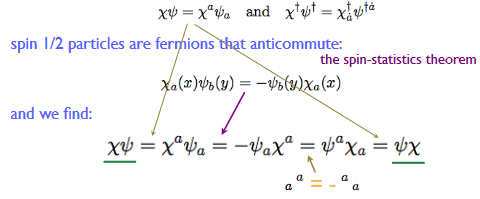
snippet grabbed from (Dermisek 09)
We analyze the special nature of the supergeometry space of field histories of the Dirac field a little (prop. ) below and conclude by highlighting the crucial role of supergeometry (remark below)
Proposition
(space of field histories of the Dirac field)
Let be the super-field bundle (def. ) for the Dirac field over Minkowski spacetime from example .
Then the corresponding supergeometric space of field histories
from example has the following properties:
-
For an ordinary Cartesian space (with no super-geometric thickening, def. ) there is only a single -parameterized collection of field histories, hence a single plot
and this corresponds to the zero section, hence to the trivial Dirac field
-
For a super Cartesian space () with a single super-odd dimension, then -parameterized collections of field histories
are in natural bijection with plots of sections of the bosonic-field bundle with field fiber the spin representation regarded as an ordinary vector space:
Moreover, these two kinds of plots determine the fermionic field space completely: It is in fact isomorphic, as a super vector space, to the bosonic field space shifted to odd degree (as in example ):
Proof
In the first case, the plot is a morphism of super Cartesian spaces (def. ) of the form
By definitions this is dually homomorphism of real supercommutative superalgebras
from the Grassmann algebra on the dual vector space of the spin representation to the ordinary algebras of smooth functions on . But the latter has no elements in odd degree, and hence all the Grassmann generators need to be send to zero.
For the second case, notice that a morphism of the form
is by def. naturally identified with a morphism of the form
where the identification on the right is from example .
By the nature of Cartesian products these morphisms in turn are naturally identified with pairs of morphisms of the form
Now, as in the first point above, here the first component is uniquely fixed to be the zero morphism ; and hence only the second component is free to choose. This is precisely the claim to be shown.
Remark
(supergeometric nature of the Dirac field)
Proposition how two basic facts about the Dirac field, which may superficially seem to be in tension with each other, are properly unified by supergeometry:
-
On the one hand a field history of the Dirac field is not an ordinary section of an ordinary vector bundle. In particular its component functions anti-commute with each other, which is not the case for ordinary functions, and this is crucial for the Lagrangian density of the Dirac field to be well defined, we come to this below in example .
-
On the other hand a field history of the Dirac field is supposed to be a spinor, hence a section of a spinor bundle, which is an ordinary vector bundle.
Therefore prop. serves to shows how, even though a Dirac field is not defined to be an ordinary section of an ordinary vector bundle, it is nevertheless encoded by such an ordinary section: One says that this ordinary section is a “superfield-component” of the Dirac field, the one linear in a Grassmann variable .
This concludes our discussion of the concept of fields itself. In the following chapter we consider the variational calculus of fields.
Field variations
In this chapter we discuss these topics:
Given a field bundle as in def. above, then we know what type of quantities the corresponding field histories assign to a given spacetime point (a given event). Among all consistent such field histories, some are to qualify as those that “may occur in reality” if we think of the field theory as a means to describe parts of the observable universe. Moreover, if the reality to be described does not exhibit “action at a distance” then admissibility of its field histories should be determined over arbitrary small spacetime regions, in fact over the infinitesimal neighbourhood of any spacetime point (remark below). This means equivalently that the realized field histories should be those that satisfy a given differential equation, namely an equation between the partial derivatives of the field history at any spacetime point. This is called the equation of motion of the field theory (def. below).
In order to formalize this, it is useful to first collect all the possible partial derivatives that a field history may have at any given point into one big space of “field derivatives at spacetime points”. This collection is called the jet bundle of the field bundle, given as def. below.
Moving around in this space means to change the possible value of fields and their derivatives, hence to vary the fields. Accordingly variational calculus of fields is just differential calculus on the jet bundle of the field bundle, this we consider in def. below.
Definition
(jet bundle of a trivial vector bundle over Minkowski spacetime)
Given a field fiber super vector space with linear basis , then for a natural number, the order- jet bundle
over Minkowski spacetime of the trivial vector bundle
is the super Cartesian space (def. ) which is spanned by coordinate functions to be denoted as follows:
where the indices range from 0 to , while the index ranges from to for the even field coordinates, and then from to for the odd-graded field coordinates and the lower indices are symmetric:
In terms of these coordinates the bundle projection map is just the one that remembers the spacetime coordinates and forgets the values of the field and its derivatives . Similarly there are intermediate projection maps
given by forgetting coordinates with more indices.
The infinite-order jet bundle
is the direct limit of super smooth sets (def. ) over these finite order jet bundles. Explicitly this means that it is the smooth set which is defined by the fact that a smooth function (a plot, by prop. )
from some super Cartesian space is equivalently a system of ordinary smooth functions into all the finite-order jet spaces
such that this system is compatible with the above projection maps, i.e. such that
The coordinate functions on a jet bundle (def. ) are to be thought of as partial derivatives of components of would-be field histories . The power of the jet bundle is that it allows to disentangle relations between would-be partial derivatives of field history components in themselves from consideration of actual field histories. In traditional physics texts this is often done implicitly. We may make it fully explit by the operation of jet prolongation which reads in a field history and records all its partial derivatives in the form of a section of the jet bundle:
Definition
Let be a field bundle (def. ) which happens to be a trivial vector bundle over Minkowski spacetime as in example .
There is a smooth function from the space of sections of , the space of field histories (example ) to the space of sections of the jet bundle (def. ) which records the field and all its spacetimes derivatives:
This is called the operation of jet prolongation: is the jet prolongation of .
Remark
(jet bundle in terms of synthetic differential geometry)
In terms of the infinitesimal geometry of formal smooth sets (def. ) the jet bundle (def. ) of a field bundle has the following incarnation:
A section of the jet bundle over a point of spacetime (an event), is equivalently a section of the original field bundle over the infinitesimal neighbourhood of that point (example ):
Moreover, given a field history , hence a section of the field bundle, then its jet prolongation (def. ) is that section of the jet bundle which under the above identification is simply the restriction of to the infinitesimal neighbourhood of :
This follows with an argument as in example .
Hence in synthetic differential geometry we have:
The jet of a section at is simply the restriction of that section to the infinitesimal neighbourhood of .
(Khavkine-Schreiber 17, section 3.3)
So the canonical coordinates on the jet bundle are the spacetime-point-wise possible values of fields and field derivates, while the jet prolongation picks the actual collections of field derivatives that may occur for an actual field history.
Example
(universal Faraday tensor/field strength on jet bundle)
Consider the field bundle (def. ) of the electromagnetic field (example ) over Minkowski spacetime (def. ), i.e. the cotangent bundle (def. ) with jet coordinates (def. ). Consider the functions on the jet bundle given by the linear combinations
of the first order jets.
Then for an electromagnetic field history (“vector potential”), hence a section
with components , its jet prolongation (def. )
has components
The pullback of the functions (30) along this jet prolongation are the components of the Faraday tensor of the field (20):
More generally, for a Lie algebra and
the field bundle for Yang-Mills theory from example , consider the functions
on the jet bundle given by
where are the structure constants of the Lie algebra as in (21), and where the square brackets around the indices denote anti-symmetrization.
We may call this the universal Yang-Mills field strength, being the covariant exterior derivative of the universal Yang-Mills field history.
For the line Lie algebra and the canonical inner product on the expression (31) reduces to the universal Faraday tensor (30) for the electromagnetic field (example ).
For a field history of Yang-Mills theory, hence a Lie algebra-valued differential 1-form, then the value of this function on that field are called the components of the covariant exterior derivative or field strength
Example
(universal B-field strength on jet bundle)
Consider the field bundle (def. ) of the B-field (example ) over Minkowski spacetime (def. ) with jet coordinates (def. ). Consider the functions on the jet bundle given by the linear combinations
where in the last step we used that .
While the jet bundle (def. ) is not finite dimensional, reflecting the fact that there are arbitrarily high orders of spacetime derivatives of a field histories, it turns out that it is only very “mildly infinite dimensional” in that smooth functions on jet bundles turn out to locally depend on only finitely many of the jet coordinates (i.e. only on a finite order of spacetime derivatives). This is the content of the following prop. .
This reflects the locality of Lagrangian field theory defined over jet bundles: If functions on the jet bundle could depend on infinitely many jet coordinates, then by Taylor series expansion of fields the function at one point over spacetime could in fact depend on field history values at a different point of spacetime. Such non-local dependence is ruled out by prop. below.
In practice this means that the situation is very convenient:
-
Any given local Lagrangian density (which will define a field theory, we come to this in def. below) will locally depend on some finite number of derivatives and may hence locally be treated as living on the ordinary manifold .
-
while at the same time all formulas (such as for the Euler-Lagrange equations, def. ) work uniformly without worries about fixing a maximal order of derivatives.
Proposition
(jet bundle is a locally pro-manifold)
Given a jet bundle as in def. , then a smooth function out of it
is such that around each point of there is a neighbourhood on which it is given by a function on a smooth function on for some finite .
(see Khavkine-Schreiber 17, section 2.2 and 3.3)
Example shows that the de Rham differential (def. ) may be encoded in terms of composing jet prolongation with a suitable function on the jet bundle. More generally, jet prolongation neatly encodes (possibly non-linear) differential operators:
Definition
Let and be two smooth fiber bundles over a common base space . Then a (possibly non-linear) differential operator from sections of to sections of is a bundle morphism from the jet bundle of (def. ) to :
or rather the function between the spaces of sections of these bundles which this induces after composition with jet prolongation (def. ):
If both and are vector bundles (def. ) so that their spaces of sections canonically are vector spaces, then is called a linear differential operator if it is a linear function between these vector spaces. This means equivalently that is a linear function in jet coordinates.
Definition
(normally hyperbolic differential operator on Minkowski spacetime)
Let be a field bundle (def. ) which is a vector bundle (def. ) over Minkowski spacetime (def. ). Write for its dual vector bundle (def. )
A linear differential operator (def. )
is of second order if it has a coordinate expansion of the form
for smooth functions on .
This is called a normally hyperbolic differential operator if its principal symbol is proportional to the inverse Minkowski metric (prop./def. ) , i.e.
Definition
(formally adjoint differential operators)
Let be a smooth vector bundle (def. ) over Minkowski spacetime (def. ) and write for the dual vector bundle (def. ).
Then a pair of linear differential operators (def. ) of the form
are called formally adjoint differential operators via a bilinear differential operator
with values in differential p-forms (def. ) such that for all sections we have
where is the volume form on Minkowski spacetime (10) and where denoted the de Rham differential (def. ).
This implies by Stokes' theorem (prop. ) in the case of compact support that under an integral and are related via integration by parts.
variational calculus and the variational bicomplex
Remark
(variational calculus – replacing plain bundle morphisms by differential operators)
Various concepts in variational calculus, especially the concept of evolutionary vector fields (def. below) and gauge parameterized implicit infinitesimal gauge symmetries (def. below) follow from concepts in plain differential geometry by systematically replacing plain bundle morphisms by bundle morphisms out of the jet bundle, hence by differential operators as in def. .
Definition
(variational derivative and total spacetime derivative – the variational bicomplex)
On the jet bundle of a trivial super vector space-vector bundle over Minkowski spacetime as in def. we may consider its de Rham complex of super differential forms (def. ); we write its de Rham differential (def. ) in boldface:
Since the jet bundle unifies spacetime with field values, we want to decompose this differential into a contribution coming from forming the total derivatives of fields along spacetime (“horizontal derivatives”), and actual variation of fields at a fixed spacetime point (“vertical derivatives”):
The total spacetime derivative or horizontal derivative on is the map on differential forms on the jet bundle of the form
which on functions (i.e. on 0-forms) is defined by
and extended to all forms by the graded Leibniz rule, hence as a nilpotent derivation of degree +1.
The variational derivative or vertical derivative
is what remains of the full de Rham differential when the total spacetime derivative (horizontal derivative) is subtracted:
We may then extend the horizontal derivative from functions on the jet bundle to all differential forms on the jet bundle by declaring that
which by (36) is equivalent to
For example
This defines a bigrading on the de Rham complex of , into horizontal degree and vertical degree
such that the horizontal and vertical derivative increase horizontal or vertical degree, respectively:
This is called the variational bicomplex.
Accordingly we will refer to the differential forms on the jet bundle often as variational differential forms.
Example
(basic facts about variational calculus)
Given the jet bundle of a field bundle as in def. , then in its variational bicomplex (def. ) we have the following:
-
The spacetime total derivative (horizontal derivative) of a spacetime coordinate function coincides with its ordinary de Rham differential
which hence is a horizontal 1-form
-
Therefore the variational derivative (vertical derivative) of a spacetime coordinate function vanishes:
(39)reflective the fact that is not a field coordinate that could be varied.
-
In particular the given volume form on gives a horizontal -form on the jet bundle, which has the same coordinate expression (and which we denote by the same symbol)
-
Generally any horizontal -form is of the form
for
any smooth function of the spacetime coordinates and the field coordinates (locally depending only on a finite order of these, by prop. ).
-
In particular every horizontal -form is proportional to the above volume form
for some smooth function that may depend on all the spacetime and field coordinates.
-
The spacetimes total derivatives /horizontal derivatives) of the variational derivative (vertical derivative) of a field variable is the differential 2-form of horizontal degree 1 and vertical degree 1 given by
In words this says that “the spacetime derivative of the variation of the field is the variation of its spacetime derivative”.
The following are less trivial properties of variational differential forms:
Proposition
(pullback along jet prolongation compatible with total spacetime derivatives)
Let be a field bundle over a spacetime (def. ), with induced jet bundle (def. ).
Then for any field history, the pullback of differential forms (def. )
along the jet prolongation of (def. )
-
intertwines the de Rham differential on spacetime (def. ) with the total spacetime derivative (horizontal derivative) on the jet bundle (def. ):
-
annihilates all vertical differential forms (def. ):
Proof
The operation of pullback of differential forms along any smooth function intertwines the full de Rham differentials (prop. ). In particular we have that
This means that the second statement immediately follows from the first, by definition of the variational (vertical) derivative as the difference between the full de Rham differential and the horizontal one:
It remains to see the first statement:
Since the jet prolongation preserves the spacetime coordinates (being a section of the jet bundle) it is immediate that the claimed relation is satisfied on the horizontal basis 1-forms (example ):
Therefore it finally remains only to check the first statement on smooth functions (0-forms). So let
be a smooth function on the jet bundle. Then by the chain rule
That this is equal to follows by the very definition of the total spacetime derivative of (34).
Proposition
(horizontal variational complex of trivial field bundle is exact)
Let be a field bundle which is a trivial vector bundle over Minkowski spacetime (example ). Then the chain complex of horizontal differential forms with the total spacetime derivative (horizontal derivative) (def. )
is exact: for all the kernel of coincides with the image of in .
More explicitly, this means that not only is every horizontally exact differential form horizontally closed (which follows immediately from the fact that we have a cochain complex in the first place, hence that ), but, conversely, if satisfies , then there exists with .
(e.g. Anderson 89, prop. 4.3)
Remark
In fact the exact sequence (40) from prop. continues further to the right, as such called the Euler-Lagrange complex. The next differential is the Euler-Lagrange operator and then then next is the Helmholtz operator.
Here we do not discuss this in detail, but we encounter aspects of the exactness further to the right below in example and in prop. .
This concludes our discussion of variational calculus on the jet bundle of the field bundle. In the next chapter we apply this to Lagrangian densities on the jet bundle, defining Lagrangian field theories.
Lagrangians
In this chapter we discuss the following topics:
Given any type of fields (def. ), those field histories that are to be regarded as “physically realizable” (if we think of the field theory as a description of the observable universe) should satisfy some differential equation – the equation of motion – meaning that realizability of any field histories may be checked upon restricting the configuration to the infinitesimal neighbourhoods (example ) of each spacetime point. This expresses the physical absence of “action at a distance” and is one aspect of what it means to have a local field theory. By remark this means that equations of motion of a field theory are equations among the coordinates of the jet bundle of the field bundle.
For many field theories of interest, their differential equation of motion is not a random partial differential equations, but is of the special kind that exhibits the “principle of extremal action” (prop. below) determined by a local Lagrangian density (def. below). These are called Lagrangian field theories, and this is what we consider here.
Namely among all the variational differential forms (def. ) two kinds stand out, namley the 0-forms in – the smooth functions – and the horizontal -forms – to be called the Lagrangian densities (def. below) – since these occupy the two “corners” of the variational bicomplex (38). There is not much to say about the 0-forms, but the Lagrangian densities do inherit special structure from their special position in the variational bicomplex:
Their variational derivative uniquely decomposes as
-
the Euler-Lagrange derivative which is proportional to the variation of the fields (instead of their derivatives)
-
the total spacetime derivative of a potential for a presymplectic current .
These two terms play a pivotal role in the theory: The condition that the first term vanishes on field histories is a differential equation on field histories, called the Euler-Lagrange equation of motion (def. below). The space of solutions to this differential equation, called the on-shell space of field histories
has the interpretation of the space of “physically realizable field histories”. This is the key object of study in the following chapters. Often this is referred to as the space of classical field histories, indicating that this does not yet reflect the full quantum field theory.
Indeed, there is also the second term in the variational derivative of the Lagrangian density, the presymplectic current , and this implies a presymplectic structure on the on-shell space of field histories (def. below) which encodes deformations of the algebra of smooth functions on . This deformation is the quantization of the field theory to an actual quantum field theory, which we discuss below.
Definition
Given a field bundle over a -dimensional Minkowski spacetime as in example , then a local Lagrangian density (for the type of field thus defined) is a horizontal differential form of degree (def. ) on the corresponding jet bundle (def. ):
By example in terms of the given volume form on spacetimes, any such Lagrangian density may uniquely be written as
where the coefficient function (the Lagrangian function) is a smooth function on the spacetime and field coordinates:
where by prop. depends locally on an arbitrary but finite order of derivatives .
We say that a field bundle (def. ) equipped with a local Lagrangian density is (or defines) a prequantum Lagrangian field theory on the spacetime .
Remark
(parameterized and physical unit-less Lagrangian densities)
More generally we may consider parameterized collections of Lagrangian densities, i.e. functions
for some Cartesian space or generally some super Cartesian space.
For example all Lagrangian densities considered in relativistic field theory are naturally smooth functions of the scale of the metric (def. )
But by the discussion in remark , in physics a rescaling of the metric is interpreted as reflecting but a change of physical units of length/distance. Hence if a Lagrangian density is supposed to express intrinsic content of a physical theory, it should remain unchanged under such a change of physical units.
This is achieved by having the Lagrangian be parameterized by further parameters, whose corresponding physical units compensate that of the metric such as to make the Lagrangian density “physical unit-less”.
This means to consider parameter spaces equipped with an action of the multiplicative group of positive real numbers, and parameterized Lagrangians
Remark
(locally variational field theory and Lagrangian p-gerbe connection)
If the field bundle (def. ) is not just a trivial vector bundle over Minkowski spacetime (example ) then a Lagrangian density for a given equation of motion may not exist as a globally defined differential -form, but only as a p-gerbe connection. This is the case for locally variational field theories such as the charged particle, the WZW model and generally theories involving higher WZW terms. For more on this see the exposition at Higher Structures in Physics.
Example
(local Lagrangian density for free real scalar field on Minkowski spacetime)
Consider the field bundle for the real scalar field from example , i.e. the trivial line bundle over Minkowski spacetime.
According to def. its jet bundle has canonical coordinates
In these coordinates, the local Lagrangian density (def. ) defining the free real scalar field of mass on is
This is naturally thought of as a collection of Lagrangians smoothly parameterized by the metric and the mass . For this to be physical unit-free in the sense of remark the physical unit of the parameter must be that of the inverse metric, hence must be an inverse length according to remark This is the inverse Compton wavelength (9) and hence the physical unit-free version of the Lagrangian density for the free scalar particle is
Example
Consider the field bundle for the real scalar field from example , i.e. the trivial line bundle over Minkowski spacetime. More generally we may consider adding to the free field Lagrangian density from example some power of the field coordinate
for some number, here called the coupling constant.
The interacting Lagrangian field theory defined by the resulting Lagrangian density
is usually called just phi^n theory.
Example
(local Lagrangian density for free electromagnetic field)
Consider the field bundle for the electromagnetic field on Minkowski spacetime from example , i.e. the cotangent bundle, which over Minkowski spacetime happens to be a trivial vector bundle of rank . With fiber coordinates taken to be , the induced fiber coordinates on the corresponding jet bundle (def. ) are .
Consider then the local Lagrangian density (def. ) given by
where are the components of the universal Faraday tensor on the jet bundle from example .
This is the Lagrangian density that defines the Lagrangian field theory of free electromagnetism.
Here for an electromagnetic field history (vector potential), then the pullback of along its jet prolongation (def. ) is the corresponding component of the Faraday tensor (20):
It follows that the pullback of the Lagrangian (43) along the jet prologation of the electromagnetic field is
Here denotes the Hodge star operator of Minkowski spacetime.
More generally:
Example
(Lagrangian density for Yang-Mills theory on Minkowski spacetime)
Let be a finite dimensional Lie algebra which is semisimple. This means that the Killing form invariant polynomial
is a non-degenerate bilinear form. Examples include the special unitary Lie algebras .
Then for the field bundle for Yang-Mills theory as in example , the Lagrangian density (def. ) -Yang-Mills theory on Minkowski spacetime is
where
is the universal Yang-Mills field strength (31).
For the purposes of perturbative quantum field theory (to be discussed below in chapter 15. Interacting quantum fields) we may allow for a rescaling of the structure constants by (at this point) a real number , to be called the coupling constant, and decompose the Lagrangian into a sum of a free field theory Lagrangian (def. ) and an interaction term:
Notice that is equivalently a sum of -copies of the Lagrangian for the electromagnetic field (example ).
On the other hand, for the purpose of exhibiting “non-perturbative effects due to instantons” in Yang-Mills theory, one consider the rescaled Yang-Mills field coordinate
with corresponding field strength
In terms of this the expression for the Lagrangian is brought back to the abstract form it had before rescaling the structure constants by the coupling constant, up to a global rescaling of all terms by the inverse square of the coupling constant:
Example
(local Lagrangian density for free B-field)
Consider the field bundle for the B-field on Minkowski spacetime from example . With fiber coordinates taken to be with
the induced fiber coordinates on the corresponding jet bundle (def. ) are .
Consider then the local Lagrangian density (def. ) given by
where are the components of the universal B-field strength on the jet bundle from example .
Example
(Lagrangian density for free Dirac field on Minkowski spacetime)
For Minkowski spacetime of dimension (def. ), consider the field bundle for the Dirac field from example . With the two-component spinor field fiber coordinates from remark , the jet bundle has induced fiber coordinates as follows:
All of these are odd-graded elements (def. ) in a Grassmann algebra (example ), hence anti-commute with each other, in generalization of (28):
The Lagrangian density (def. ) of the massless free Dirac field on Minkowski spacetime is
given by the bilinear pairing from prop. of the field coordinate with its first spacetime derivative and expressed here in two-component spinor field coordinates as in (15), hence with the Dirac conjugate (14) on the left.
Specifically in spacetime dimension , the Lagrangian function for the massive Dirac field of mass is
This is naturally thought of as a collection of Lagrangians smoothly parameterized by the metric and the mass . For this to be physical unit-free in the sense of remark the physical unit of the parameter must be that of the inverse metric, hence must be an inverse length according to remark This is the inverse Compton wavelength (9) and hence the physical unit-free version of the Lagrangian density for the free Dirac field is
Remark
(reality of the Lagrangian density of the Dirac field)
The kinetic term of the Lagrangian density for the Dirac field form def. is a sum of two contributions, one for each chiral spinor component in the full Dirac spinor (remark ):
Here the computation shown under the brace crucially uses that all these jet coordinates for the Dirac field are anti-commuting, due to their supergeometric nature (46).
Notice that a priori this is a function on the jet bundle with values in . But in fact for it is real up to a total spacetime derivative:, because
and similarly for
(e.g. Dermisek I-9)
Example
(Lagrangian density for quantum electrodynamics)
Consider the fiber product of the field bundles for the electromagnetic field (example ) and the Dirac field (example ) over 4-dimensional Minkowski spacetime (def. ):
This means that now a field history is a pair , with a field history of the electromagnetic field and a field history of the Dirac field.
On the resulting jet bundle consider the Lagrangian density
for some number, called the coupling constant. This is called the electron-photon interaction.
Then the sum of the Lagrangian densities for
-
the free electromagnetic field (example );
-
the free Dirac field (example )
-
the above electron-photon interaction
defines the interacting field theory Lagrangian field theory whose perturbative quantization is called quantum electrodynamics.
In this context the square of the coupling constant
is called the fine structure constant.
Euler-Lagrange forms and presymplectic currents
The beauty of Lagrangian field theory (def. ) is that a choice of Lagrangian density determines both the equations of motion of the fields as well as a presymplectic structure on the space of solutions to this equation (the “shell”), making it the “covariant phase space” of the theory. All this we discuss below. But in fact all this key structure of the field theory is nothing but the shadow (under “transgression of variational differential forms”, def. below) of the following simple relation in the variational bicomplex:
Proposition
(Euler-Lagrange form and presymplectic current)
Given a Lagrangian density as in def. , then its de Rham differential , which by degree reasons equals , has a unique decomposition as a sum of two terms
such that is proportional to the variational derivative of the fields (but not their derivatives, called a “source form”):
The map
thus defined is called the Euler-Lagrange operator and is explicitly given by the Euler-Lagrange derivative:
The smooth subspace of the jet bundle on which the Euler-Lagrange form vanishes
is called the shell. The smaller subspace on which also all total spacetime derivatives vanish (the “formally integrable prolongation”) is the prolonged shell
Saying something holds “on-shell” is to mean that it holds after restriction to this subspace. For example a variational differential form is said to vanish on shell if .
The remaining term in (49) is unique, while the presymplectic potential
is not unique.
(For a field bundle which is a trivial vector bundle (example over Minkowski spacetime (def. ), prop. says that is unique up to addition of total spacetime derivatives , for .)
One possible choice for the presymplectic current is
where
denotes the contraction (def. ) of the volume form with the vector field .
The vertical derivative of a chosen presymplectic potential is called a pre-symplectic current for :
Given a choice of then the sum
is called the corresponding Lepage form. Its de Rham derivative is the sum of the Euler-Lagrange variation and the presymplectic current:
(Its conceptual nature will be elucidated after the introduction of the local BV-complex in example below.)
Proof
Using and that by degree reasons (example ), we find
The idea now is to have pick up those terms that would appear as boundary terms under the integral if we were to consider integration by parts to remove spacetime derivatives of .
We compute, using example , the total horizontal derivative of from (54) as follows:
where in the last line we used that
Here the two terms proportional to cancel out, and we are left with
Hence shares with the terms that are proportional to for , and so the remaining terms are proportional to , as claimed:
The following fact is immediate from prop. , but of central importance, we futher amplify this in remark below:
Proposition
(total spacetime derivative of presymplectic current vanishes on-shell)
Let be a Lagrangian field theory (def. ). Then the Euler-Lagrange form and the presymplectic current (prop. ) are related by
In particular this means that restricted to the prolonged shell (52) the total spacetime derivative of the presymplectic current vanishes:
Proof
The claim follows from applying the variational derivative to both sides, using (37): and .
Many examples of interest fall into the following two special cases of prop. :
Example
(Euler-Lagrange form for spacetime-independent Lagrangian densities)
Let be a Lagrangian field theory (def. ) whose field bundle is a trivial vector bundle over Minkowski spacetime (example ).
In general the Lagrangian density is a function of all the spacetime and field coordinates
Consider the special case that is spacetime-independent in that the Lagrangian function is independent of the spacetime coordinate . Then the same evidently holds for the Euler-Lagrange form (prop. ). Therefore in this case the shell (52) is itself a trivial bundle over spacetime.
In this situation every point in the jet fiber defines a constant section of the shell:
Example
Consider a Lagrangian field theory (def. ) whose Lagrangian density
-
does not depend on the spacetime-coordinates (example );
-
depends on spacetime derivatives of field coordinates (hence on jet bundle coordinates) at most to first order.
Hence if the field bundle is a trivial vector bundle over Minkowski spacetime (example ) this means to consider the case that
Then the presymplectic current (def. ) is (up to possibly a horizontally exact part) of the form
where
denotes the partial derivative of the Lagrangian function with respect to the spacetime-derivatives of the field coordinates.
Here
is called the canonical momentum corresponding to the “canonical field coordinate” .
In the language of multisymplectic geometry the full expression
is also called the “canonical multi-momentum”, or similar.
Proof
We compute:
Hence
Remark
(presymplectic current is local version of (pre-)symplectic form of Hamiltonian mechanics)
In the simple but very common situation of example the presymplectic current (def. ) takes the form (61)
with the field coordinates (“canonical coordinates”) and the “canonical momentum” (61).
Notice that this is of the schematic form “”, which is reminiscent of the wedge product of a symplectic form expressed in Darboux coordinates with a volume form for a -dimensional manifold. Indeed, below in Phase space we discuss that this presymplectic current “transgresses” (def. below) to a presymplectic form of the schematic form “” on the on-shell space of field histories (def. ) by integrating it over a Cauchy surface of dimension . In good situations this presymplectic form is in fact a symplectic form on the on-shell space of field histories (theorem below).
This shows that the presymplectic current is the local (i.e. jet level) avatar of the symplectic form that governs the formulation of Hamiltonian mechanics in terms of symplectic geometry.
In fact prop. may be read as saying that the presymplectic current is a conserved current (def. below), only that it takes values not in smooth functions of the field coordinates and jets, but in variational 2-forms on fields. There is a conserved charge associated with every conserved current (prop. below) and the conserved charge associated with the presymplectic current is the (pre-)symplectic form on the phase space of the field theory (def. below).
Example
(Euler-Lagrange form and presymplectic current for free real scalar field)
Consider the Lagrangian field theory of the free real scalar field from example .
Then the Euler-Lagrange form and presymplectic current (prop. ) are
and
respectively.
Proof
This is a special case of example , but we spell it out in detail again:
We need to show that Euler-Lagrange operator takes the local Lagrangian density for the free scalar field to
First of all, using just the variational derivative (vertical derivative) is a graded derivation, the result of applying it to the local Lagrangian density is
By definition of the Euler-Lagrange operator, in order to find and , we need to exhibit this as the sum of the form .
The key to find is to realize as a total spacetime derivative (horizontal derivative). Since this is accomplished by
where on the right we have the contraction (def. ) of the tangent vector field along into the volume form.
Hence we may take the presymplectic potential (53) of the free scalar field to be
because with this we have
In conclusion this yields the decomposition of the vertical differential of the Lagrangian density
which shows that is as claimed, and that is a presymplectic potential current (53). Hence the presymplectic current itself is
Example
(Euler-Lagrange form for free electromagnetic field)
Consider the Lagrangian field theory of free electromagnetism from example .
The Euler-Lagrange variational derivative is
Proof
By (50) we have
More generally:
Example
(Euler-Lagrange form for Yang-Mills theory on Minkowski spacetime)
Let be a semisimple Lie algebra and consider the Lagrangian field theory of -Yang-Mills theory from example .
Its Euler-Lagrange form (prop. ) is
where
is the universal Yang-Mills field strength (31).
Proof
With the explicit form (50) for the Euler-Lagrange derivative we compute as follows:
In the last step we used that for a semisimple Lie algebra is totally skew-symmetric in its indices (this being the coefficients of the Lie algebra cocycle) which is in transgression with the Killing form invariant polynomial .
Example
(Euler-Lagrange form of free B-field)
Consider the Lagrangian field theory of the free B-field from example .
The Euler-Lagrange variational derivative is
where is the universal B-field strength from example .
Proof
By (50) we have
Example
(Euler-Lagrange form and presymplectic current of Dirac field)
Consider the Lagrangian field theory of the Dirac field on Minkowski spacetime of dimension (example ).
Then
-
the Euler-Lagrange variational derivative (def. ) in the case of vanishing mass is
and in the case that spacetime dimension is and arbitrary mass , it is
-
its presymplectic current (def. ) is
Proof
In any case the canonical momentum of the Dirac field according to example is
This yields the presymplectic current as claimed, by example .
Now regarding the Euler-Lagrange form, first consider the massless case in spacetime dimension , where
Then we compute as follows:
Here the first equation is the general formula (50) for the Euler-Lagrange variation, while the identity under the braces combines two facts (as in remark above):
-
the symmetry (12) of the spinor pairing (prop. );
-
the anti-commutativity (46) of the Dirac field and jet coordinates, due to their supergeometric nature (remark ).
Finally in the special case of the massive Dirac field in spacetime dimension the Lagrangian function is
where now takes values in the complex numbers (as opposed to in , or ). Therefore we may now form the derivative equivalently by treeating and as independent components of the field. This immediately yields the claim.
Example
(trivial Lagrangian densities and the Euler-Lagrange complex)
If a Lagrangian density (def. ) is in the image of the total spacetime derivative, hence horizontally exact (def. )
for any , then both its Euler-Lagrange form as well as its presymplectic current (def. ) vanish:
This is because with (37) the defining unique decomposition (49) of is given by
which then implies with (55) that
Therefore the Lagrangian densities which are total spacetime derivatives are also called trivial Lagrangian densities.
If the field bundle is a trivial vector bundle (example ) over Minkowski spacetime (def. ) then also the converse is true: Every Lagrangian density whose Euler-Lagrange form vanishes is a total spacetime derivative.
Stated more abstractly, this means that the exact sequence of the total spacetime from prop. extends to the right via the Euler-Lagrange variational derivative to an exact sequence of the form
In fact, as shown, this exact sequence keeps going to the right; this is also called the Euler-Lagrange complex.
The next differential after the Euler-Lagrange variational derivative is known as the Helmholtz operator. By definition of exact sequence, the Helmholtz operator detects whether a partial differential equation on field histories, induced by a variational differential form as in (65) comes from varying a Lagrangian density, hence whether it is the equation of motion of a Lagrangian field theory via def. .
This way homological algebra is brought to bear on core questions of field theory. For more on this see the exposition at Higher Structures in Physics.
Remark
(supergeometric nature of Lagrangian density of the Dirac field)
Observe that the Lagrangian density for the Dirac field (def. ) makes sense (only) due to the supergeometric nature of the Dirac field (remark ): If the field jet coordinates were not anti-commuting (46) then the Dirac’s field Lagrangian density (def. ) would be a total spacetime derivative and hence be trivial according to example .
This is because
Here the identification under the brace uses two facts:
-
the symmetry (12) of the spinor bilinear pairing ;
-
the anti-commutativity (46) of the Dirac field and jet coordinates, due to their supergeometric nature (remark ).
The second fact gives the minus sign under the brace, which makes the total expression vanish, if the Dirac field and jet coordinates indeed are anti-commuting (which, incidentally, means that we found an “off-shell conserved current” for the Dirac field, see example below).
If however the Dirac field and jet coordinates did commute with each other, we would instead have a plus sign under the brace, in which case the total horizontal derivative expression above would equal the massless Dirac field Lagrangian (47), thus rendering it trivial in the sense of example .
The same supergeometric nature of the Dirac field will be necessary for its intended equation of motion, the Dirac equation (example ) to derive from a Lagrangian density; see the proof of example below, and see remark below.
Euler-Lagrange equations of motion
The key implication of the Euler-Lagrange form on the jet bundle is that it induces the equation of motion on the space of field histories:
Definition
(Euler-Lagrange equation of motion)
Given a Lagrangian field theory (def. then the corresponding Euler-Lagrange equations of motion is the condition on field histories (def. )
to have a jet prolongation (def. )
that factors through the shell inclusion (51) defined by vanishing of the Euler-Lagrange form (prop. )
(This implies that factors even through the prolonged shell (52).)
In the case that the field bundle is a trivial vector bundle over Minkowski spacetime as in example this is the condition that satisfies the following differential equation (again using prop. ):
where the differential operator (def. )
from the field bundle (def. ) to its vertical cotangent bundle (def. ) is given by the Euler-Lagrange derivative (50).
The on-shell space of field histories is the space of solutions to this condition, namely the the sub-super smooth set (def. ) of the full space of field histories (22) (def. )
whose plots are those that factor through the shell (65).
More generally for a submanifold of spacetime, we write
for the sub-super smooth ste of on-shell field histories restricted to the infinitesimal neighbourhood of in (25).
Definition
A Lagrangian field theory (def. ) with field bundle a vector bundle (e.g. a trivial vector bundle as in example ) is called a free field theory if its Euler-Lagrange equations of motion (def. ) is a differential equation that is linear differential equation, in that with
any two on-shell field histories (67) and any two real numbers, also the linear combination
which a priori exists only as an element in the off-shell space of field histories, is again a solution to the equations of motion and hence an element of .
A Lagrangian field theory which is not a free field theory is called an interacting field theory.
Remark
(relevance of free field theory)
In perturbative quantum field theory one considers interacting field theories in the infinitesimal neighbourhood (example ) of free field theories (def. ) inside some super smooth set of general Lagrangian field theories. While free field theories are typically of limited interest in themselves, this perturbation theory around them exhausts much of what is known about quantum field theory in general, and therefore free field theories are of paramount importance for the general theory.
We discuss the covariant phase space of free field theories below in Propagators and their quantization below in Free quantum fields.
Example
(equation of motion of free real scalar field is Klein-Gordon equation)
Consider the Lagrangian field theory of the free real scalar field from example .
By example its Euler-Lagrange form is
Hence for a field history, its Euler-Lagrange equation of motion according to def. is
often abbreviated as
This PDE is called the Klein-Gordon equation on Minowski spacetime. If the mass vanishes, , then this is the relativistic wave equation.
Hence this is indeed a free field theory according to def. .
The corresponding linear differential operator (def. )
is called the Klein-Gordon operator.
For later use we record the following basic fact about the Klein-Gordon equation:
Example
(Klein-Gordon operator is formally self-adjoint )
The Klein-Gordon operator (70) is its own formal adjoint (def. ) witnessed by the bilinear differential operator (33) given by
Proof
Example
(equations of motion of vacuum electromagnetism are vacuum Maxwell's equations)
Consider the Lagrangian field theory of free electromagnetism on Minkowski spacetime from example .
By example its Euler-Lagrange form is
Hence for a field history (“vector potential”), its Euler-Lagrange equation of motion according to def. is
where is the Faraday tensor (20). (In the coordinate-free formulation in the second line “” denotes the Hodge star operator induced by the pseudo-Riemannian metric on Minkowski spacetime.)
These PDEs are called the vacuum Maxwell's equations.
This, too, is a free field theory according to def. .
Example
(equation of motion of Dirac field is Dirac equation)
Consider the Lagrangian field theory of the Dirac field on Minkowski spacetime from example , with field fiber the spin representation regarded as a superpoint and Lagrangian density given by the spinor bilinear pairing
(in spacetime dimension with unless ).
By example the Euler-Lagrange differential operator (66) for the Dirac field is of the form
so that the corresponding Euler-Lagrange equation of motion (def. ) is equivalently
This is the Dirac equation and is called a Dirac operator. In terms of the Feynman slash notation from (16) the corresponding differential operator, the Dirac operator reads
Hence this is a free field theory according to def. .
Observe that the “square” of the Dirac operator is the Klein-Gordon operator (69)
This means that a Dirac field which solves the Dirac equations is in particular (on Minkowski spacetime) componentwise a solution to the Klein-Gordon equation.
Remark
(supergeometric nature of the Dirac equation as an Euler-Lagrange equation)
While the Dirac equation (73) of example would make sense in itself also if the field coordinates and jet coordinates of the Dirac field were not anti-commuting (46), due to their supergeometric nature (remark ), it would, by remark , then no longer be the Euler-Lagrange equation of a Lagrangian density, hence then Dirac field theory would not be a Lagrangian field theory.
Example
(Dirac operator on Dirac spinors is formally self-adjoint differential operator)
The Dirac operator, hence the differential operator corresponding to the Dirac equation of example via def. is a formally anti-self adjoint (def. ):
Proof
By (72) we are to regard the Dirac operator as taking values in the dual spin bundle by using the Dirac conjugate (14):
Then we need to show that there is such that for all pairs of spinor sections we have
But the spinor-to-vector pairing is symmetric (12), hence this is equivalent to
By the product law of differentiation, this is solved, for all , by
This concludes our discussion of Lagrangian densities and their variational calculus. In the next chapter we consider the infinitesimal symmetries of Lagrangians and the conserved currents that these induce via Noether's theorem.
Symmetries
In this chapter we discuss these topics:
We have introduced the concept of Lagrangian field theories in terms of a field bundle equipped with a Lagrangian density on its jet bundle (def. ). Generally, given any object equipped with some structure, it is of paramount interest to determine the symmetries, hence the isomorphisms/equivalences of the object that preserve the given structure (this is the “Erlanger program”, Klein 1872).
The infinitesimal symmetries of the Lagrangian density (def. below) send one field history to an infinitesimally nearby one which is “equivalent” for all purposes of field theory. Among these are the infinitesimal gauge symmetries which will be of concern below. A central theorem of variational calculus says that infinitesimal symmetries of the Lagrangian correspond to conserved currents, this is Noether's theorem I, prop. below. These conserved currents constitute an extension of the Lie algebra of symmetries, called the Dickey bracket.
But in (57) we have seen that the Lagrangian density of a Lagrangian field theory is just one component, in codimension 0, of an inhomogeneous “Lepage form” which in codimension 1 is given by the presymplectic potential current (53). (This will be conceptually elucidated, after we have introduced the local BV-complex, in example below.) This means that in codimension 1 we are to consider infinitesimal on-shell symmetries of the Lepage form . These are known as Hamiltonian vector fields (def. below) and the analog of Noether's theorem I now says that these correspond to Hamiltonian differential forms. The Lie algebra of these infinitesimal symmetries is called the local Poisson bracket (prop. below).
Noether theorem and Hamiltonian Noether theorem
| variational form | symmetry | homotopy formula | physical quantity | local symmetry algebra |
|---|---|---|---|---|
| Lagrangian density (def. ) | conserved current (def. ) | Dickey bracket | ||
| presymplectic current (prop. ) | Hamiltonian form (def. ) | local Poisson bracket (prop. ) |
In the chapter Phase space below we transgress this local Poisson bracket of infinitesimal symmetries of the presymplectic potential current to the “global” Poisson bracket on the covariant phase space (def. below). This is the structure which then further below leads over to the quantization (deformation quantization) of the prequantum field theory to a genuine perturbative quantum field theory. However, it will turn out that there may be an obstruction to this construction, namely the existence of special infinitesimal symmetries of the Lagrangian densities, called implicit gauge symmetries (discussed further below).
infinitesimal symmetries of the Lagrangian density
Definition
(variation)
Let be a field bundle (def. ).
A variation is a vertical vector field on the jet bundle (def. ) hence a vector field which vanishes when evaluated in the horizontal differential forms.
In the special case that the field bundle is trivial vector bundle over Minkowski spacetime as in example , a variation is of the form
The concept of variation in def. is very general, in that it allows to vary the field coordinates independently from the corresponding jets. This generality is necessary for discussion of symmetries of presymplectic currents in def. below. But for discussion of symmetries of Lagrangian densities we are interested in explicitly varying just the field coordinates (def. below) and inducing from this the corresponding variations of the field derivatives (prop. ) below.
In order to motivate the following definition of evolutionary vector fields we follow remark saying that concepts in variational calculus are obtained from their analogous concepts in plain differential calculus by replacing plain bundle morphisms by morphisms out of the jet bundle:
Given a fiber bundle , then a vertical vector field on is a section of its vertical tangent bundle (def. ), hence is a bundle morphism of this form
The variational version replaces the vector bundle on the left with its jet bundle:
Definition
Let be a field bundle (def. ). Then an evolutionary vector field on is “variational vertical vector field” on , hence a smooth bundle homomorphism out of the jet bundle (def. )
to the vertical tangent bundle (def. ) of .
In the special case that the field bundle is a trivial vector bundle over Minkowski spacetime as in example , this means that an evolutionary vector field is a tangent vector field (example ) on of the special form
where the coefficients are general smooth functions on the jet bundle (while the cmponents are tangent vectors along the field coordinates , but not along the spacetime coordinates and not along the jet coordinates ).
We write
for the space of evolutionary vector fields, regarded as a module over the -algebra
of smooth functions on the jet bundle.
An evolutionary vector field (def. ) describes an infinitesimal change of field values depending on, possibly, the point in spacetime and the values of the field and all its derivatives (locally to finite order, by prop. ).
This induces a corresponding infinitesimal change of the derivatives of the fields, called the prolongation of the evolutionary vector field:
Proposition
(prolongation of evolutionary vector field)
Let be a fiber bundle.
Given an evolutionary vector field on (def. ) there is a unique tangent vector field (example ) on the jet bundle (def. ) such that
-
agrees on field coordinates (as opposed to jet coordinates) with :
which means in the special case that is a trivial vector bundle over Minkowski spacetime (example ) that is of the form
(74) -
contraction with (def. ) anti-commutes with the total spacetime derivative (def. ):
(75)
In particular Cartan's homotopy formula (prop. ) for the Lie derivative holds with respect to the variational derivative :
Explicitly, in the special case that the field bundle is a trivial vector bundle over Minkowski spacetime (example ) is given by
Proof
It is sufficient to prove the coordinate version of the statement. We prove this by induction over the maximal jet order . Notice that the coefficient of in is given by the contraction (def. ).
Similarly (at “”) the component of is given by . But by the second condition above this vanishes:
Moreover, the coefficient of in is fixed by the first condition above to be
This shows the statement for . Now assume that the statement is true up to some . Observe that the coefficients of all are fixed by the contractions with . For this we find again from the second condition and using as well as the induction assumption that
This shows that satisfying the two conditions given exists uniquely.
Finally formula (76) for the Lie derivative follows from the second of the two conditions with Cartan's homotopy formula (prop. ) together with (35).
Proposition
(evolutionary vector fields form a Lie algebra)
Let be a fiber bundle. For any two evolutionary vector fields , on (def. ) the Lie bracket of tangent vector fields of their prolongations , (def. ) is itself the prolongation of a unique evolutionary vector field .
This defines the structure of a Lie algebra on evolutionary vector fields.
Proof
It is clear that is still vertical, therefore, by prop. , it is sufficient to show that contraction with this vector field (def. ) anti-commutes with the horizontal derivative , hence that .
Now is an operator that sends vertical 1-forms to horizontal 1-forms and vanishes on horizontal 1-forms. Therefore it is sufficient to see that this operator in fact also vanishes on all vertical 1-forms. But for this it is sufficient that it commutes with the vertical derivative. This we check by Cartan calculus, using and , by assumption:
Now given an evolutionary vector field, we want to consider the flow that it induces on the space of field histories:
Definition
(flow of field histories along evolutionary vector field)
Let be a field bundle (def. ) and let be an evolutionary vector field (def. ) such that the ordinary flow of its prolongation (prop. )
exists on the jet bundle (e.g. if the order of derivatives of field coordinates that it depends on is bounded).
For a collection of field histories (hence a plot of the space of field histories (def. ) ) the flow of through is the smooth function
whose unique factorization through the space of jets of field histories (i.e. the image of jet prolongation, def. )
takes a plot of the real line (regarded as a super smooth set via example ), to the plot
of the smooth space of sections of the jet bundle.
(That indeed flows jet prolongations again to jet prolongations is due to its defining relation to the evolutionary vector field from prop. .)
Definition
(infinitesimal symmetries of the Lagrangian and conserved currents)
Let be a Lagrangian field theory (def. ).
Then
-
an infinitesimal symmetry of the Lagrangian is an evolutionary vector field (def. ) such that the Lie derivative of the Lagrangian density along its prolongation (prop. ) is a total spacetime derivative:
-
an on-shell conserved current is a horizontal -form (def. ) whose total spacetime derivative vanishes on the prolonged shell (51)
Proposition
Let be a Lagrangian field theory (def. ).
If is an infinitesimal symmetry of the Lagrangian (def. ) with , then
is an on-shell conserved current (def. ), for a presymplectic potential (53) from def. .
(Noether's theorem II is prop. below.)
Proof
By Cartan's homotopy formula for the Lie derivative (prop. ) and the decomposition of the variational derivative (49) and the fact that contraction with the prolongtion of an evolutionary vector field vanishes on horizontal differential forms (74) and anti-commutes with the horizontal differential (75), by def. , we may re-express the defining equation for the symmetry as follows:
which is equivalent to
Since, by definition of the shell , the differential form on the right vanishes on this yields the claim.
Example
(energy-momentum of the scalar field)
Consider the Lagrangian field theory of the free scalar field from def. :
For consider the vector field on the jet bundle given by
This describes infinitesimal translations of the fields in the direction of .
And this is an infinitesimal symmetry of the Lagrangian (def. ), since
With the formula (63) for the presymplectic potential
it hence follows from Noether's theorem (prop. ) that the corresponding conserved current (def. ) is
This conserved current is called the energy-momentum tensor.
Example
Consider the Lagrangian field theory of the free Dirac field on Minkowski spacetime in spacetime dimension (example )
Then the prolongation (prop. ) of the evolutionary vector field (def. )
is an infinitesimal symmetry of the Lagrangian (def. ). The conserved current that corresponds to this under Noether's theorem I (prop. ) is
This is called the Dirac current.
Proof
By equation (77) the prolongation of is
Therefore the Lagrangian density is strictly invariant under the Lie derivative along
and so the formula for the corresponding conserved current (79) is
where under the brace we used example to identify the presymplectic potential for the free Dirac field.
Since an infinitesimal symmetry of a Lagrangian (def. ) by definition changes the Lagrangian only up to a total spacetime derivative, and since the Euler-Lagrange equations of motion by construction depend on the Lagrangian density only up to a total spacetime derivative (prop. ), it is plausible that and infinitesimal symmetry of the Lagrangian preserves the equations of motion (50), hence the shell (52). That this is indeed the case is the statement of prop. below.
To make the proof transparent, we now first introduce the concept of the evolutionary derivative (def. ) below and then observe that in terms of these the Euler-Lagrange derivative is in fact a derivation (prop. ).
Definition
For
a fiber bundle (def. ), regarded as a field bundle (def. ), and for
any other fiber bundle over the same base space (spacetime), we write
for the space of sections of the pullback of bundles of to the jet bundle (def. ) along .
(Equivalently this is the space of differential operators from sections of to sections of , according to prop. . )
In (Olver 93, section 5.1, p. 288) the field dependent sections of def. , considered in local coordinates, are referred to as tuples of differential functions.
Example
(source forms and evolutionary vector fields are field-dependent sections)
For a field bundle, write for its vertical tangent bundle (example ) and for its dual vector bundle (def. ), the vertical cotangent bundle.
Then the field-dependent sections of these bundles according to def. are identified as follows:
-
the space contains the space of evolutionary vector fields (def. ) as those bundle morphism which respect not just the projection to but also its factorization through :
-
contains the space of source forms (prop. ) as those bundle morphisms which respect not just the projection to but also its factorization through :
This makes manifest the duality pairing between source forms and evolutionary vector fields
which in local coordinates is given by
for smooth functions on the jet bundle (as in prop. ).
Definition
(evolutionary derivative of field-dependent section)
Let
be a fiber bundle regarded as a field bundle (def. ) and let
be a vector bundle (def. ). Then for
a field-dependent section of according to def. , its evolutionary derivative is the morphism
which, under the identification of example , sense an evolutionary vector field to the derivative of (example ) along the prolongation tangent vector field of (prop. ).
In the case that and are trivial vector bundles over Minkowski spacetime with coordinates and , respectively (example ), then by (77) this is given by
This makes manifest that may equivalently be regarded as a -dependent differential operator (def. ) from the vertical tangent bundle (def. ) to , namely a bundle homomorphism over of the form
in that
Example
(evolutionary derivative of Lagrangian function)
Over Minkowski spacetime (def. ), let be a Lagrangian density (def. ), with coefficient function regarded as a field-dependent section (def. ) of the trivial real line bundle:
Then the formally adjoint differential operator (def. )
of its evolutionary derivative, def. , regarded as a -dependent differential operator from to and applied to the constant section
is the Euler-Lagrange derivative (50)
Proposition
(Euler-Lagrange derivative is derivation via evolutionary derivatives)
Let be a vector bundle (def. ) and write for its dual vector bundle (def. ).
For field-dependent sections (def. )
and
we have that the Euler-Lagrange derivative (50) of their canonical pairing to a smooth function on the jet bundle (as in prop. ) is the sum of the derivative of either one via the formally adjoint differential operator (def. ) of the evolutionary derivative (def. ) of the other:
Proof
It is sufficient to check this in local coordinates. By the product law for differentiation we have
Proposition
(evolutionary derivative of Euler-Lagrange forms is formally self-adjoint)
Let be a Lagrangian field theory (def. ) over Minkowski spacetime (def. ) and regard the Euler-Lagrange derivative
(from prop. ) as a field-dependent section of the vertical cotangent bundle
as in example . Then the corresponding evolutionary derivative field-dependent differential operator (def. ) is formally self-adjoint (def. ):
(In terms of the Euler-Lagrange complex, remark , this says that the Helmholtz operator vanishes on the image of the Euler-Lagrange operator.)
(Olver 93, theorem 5.92) The following proof is due to Igor Khavkine.
Proof
By definition of the Euler-Lagrange form (def. ) we have
Applying the variational derivative (def. ) to both sides of this equation yields
It follows that for any two evolutionary vector fields the contraction (def. ) of their prolongations and (def. ) into the differential 2-form on the left is
by inspection of the definition of the evolutionary derivative (def. ). Moreover, their contraction into the differential form on the right is
by the fact (prop. ) that contraction with prolongations of evolutionary vector fields anti-commutes with the total spacetime derivative (75).
Hence the last two equations combined give
This is the defining condition for to be formally self-adjoint differential operator (def. ).
Now we may finally prove that an infinitesimal symmetry of the Lagrangian is also an infinitesimal symmetry of the Euler-Lagrange equations of motion:
Proposition
(infinitesimal symmetries of the Lagrangian are also infinitesimal symmetries of the equations of motion)
Let be a Lagrangian field theory. If an evolutionary vector field is an infinitesimal symmetry of the Lagrangian then the flow along its prolongation preserves the prolonged shell (52) in that the Lie derivative of the Euler-Lagrange form along vanishes on :
Proof
Notice that for any vector field the Lie derivative (prop. ) of the Euler-Lagrange form differs from that of its component functions by a term proportional to these component functions, which by definition vanishes on-shell:
But the Lie derivative of the component functions is just their plain derivative. Therefore it is sufficient to show that
Now by Noether's theorem I (prop. ) the condition for an infinitesimal symmetry of the Lagrangian implies that the contraction (def. ) of the Euler-Lagrange form with the corresponding evolutionary vector field is a total spacetime derivative:
Since the Euler-Lagrange derivative vanishes on total spacetime derivative (example ) also its application on the contraction on the left vanishes. But via example that contraction is a pairing of field-dependent sections as in prop. . Hence we use this proposition to compute:
Here the first step is by prop. , the second step is by prop. and the third step is (81).
Hence
where in the last line we used that on the prolonged shell and all its horizontal derivatives vanish, by definition.
As a corollary we obtain:
Proposition
(flow along infinitesimal symmetry of the Lagrangian preserves on-shell space of field histories)
Let be a Lagrangian field theory (def. ).
For an infinitesimal symmetry of the Lagrangian (def. ) the flow on the space of field histories (example ) that it induces by def. preserves the space of on-shell field histories (from prop. ):
Proof
By def. a field history is on-shell precisely if its jet prolongation (def. ) factors through the shell (51). Hence by def. the statement is equivalently that the ordinary flow (prop. ) of (def. ) on the jet bundle preserves the shell. This in turn means that it preserves the vanishing locus of the Euler-Lagrange form , which is the case by prop. .
infinitesimal symmetries of the presymplectic potential current
Evidently Noether's theorem I in variational calculus (prop. ) is the special case for horizontal -forms of a more general phenomenon relating symmetries of variational forms to forms that are closed up to a contraction. The same phenomenon applied instead to the presymplectic current yields the following:
Definition
(variational Lie derivative)
Let be a field bundle (def. ) with jet bundle (def. ).
For a vertical tangent vector field on the jet bundle (a variation def. ) write
for the variational Lie derivative along , analogous to Cartan's homotopy formula (prop. ) but defined in terms of the variational derivative (35) as opposed to the full de Rham differential.
Then for and two vertical vector fields, write
for the vector field whose contraction operator (def. ) is given by
Definition
(infinitesimal symmetry of the presymplectic potential and Hamiltonian differential forms)
Let be a Lagrangian field theory (def. ) with presymplectic potential current (53). Write for the shell (51).
Then:
-
An on-shell variation (def. ) is an infinitesimal symmetry of the presymplectic current or Hamiltonian vector field if on-shell (def. ) its variational Lie derivative along (def. ) is a variational derivative:
for some variational form .
-
A Hamiltonian differential form (or local Hamiltonian current) is a variational form on the shell such that there exists a variation with
We write
for the space of pairs consisting of a Hamiltonian differential forms on-shell and a corresponding variation.
Proposition
(Hamiltonian Noether's theorem)
A variation is an infinitesimal symmetry of the presymplectic potential (def. ) with precisely if
is a Hamiltonian differential form for .
Since therefore both the conserved currents from Noether's theorem as well as the Hamiltonian differential forms are generators of infinitesimal symmetries of certain variational forms (namely of the Lagrangian density and of the presymplectic current, respectively) they form a Lie algebra. For the conserved currents this is sometimes known as the Dickey bracket Lie algebra. For the Hamiltonian forms it is the Poisson bracket Lie p+1-algebra. Since here for simplicity we are considering just vertical variations, we have just a plain Lie algebra. The transgression of this Lie algebra of Hamiltonian forms on the jet bundle to Cauchy surfaces yields a presymplectic structure on phase space, this we discuss below.
Proposition
Let be a Lagrangian field theory (def. ).
On the space pairs of Hamiltonian differential forms with compatible variation (def. ) the following operation constitutes a Lie bracket:
where is the variational Lie bracket from def. .
We call this the local Poisson Lie bracket.
Proof
First we need to check that the bracket is well defined in itself. It is clear that it is linear and skew-symmetric, but what needs proof is that it does indeed land in , hence that the following equation holds:
With def. for and we compute this as follows:
This shows that the bracket is well defined.
It remains to see that the bracket satifies the Jacobi identity:
hence that
Here holds because by def. acts as a derivation, and hence what remains to be shown is that
We check this by repeated uses of def. , using in addition that
-
(since by being Hamiltonian)
-
(since in addition )
-
(since is of vertical degree 2, and since all variations are vertical by assumption).
So we compute as follows (a special case of FRS 13b, lemma 3.1.1):
The local Poisson bracket Lie algebra from prop. is but the lowest stage of a higher Lie theoretic structure called the Poisson bracket Lie p-algebra. Here we will not go deeper into this higher structure (see at Higher Prequantum Geometry for more), but below we will need the following simple shadow of it:
Lemma
The horizontally exact Hamiltonian forms constitute a Lie ideal for the local Poisson Lie bracket (84).
Proof
Let be a horizontally exact Hamiltonian form, hence
for some . Write for a Hamiltonian vector field for .
Then for any other pair consisting of a Hamiltonian form and a corresponding Hamiltonian vector field, we have
Here we used that the horizontal derivative anti-commutes with the vertical one by construction of the variational bicomplex, and that anti-commutes with the horizontal derivative since the variation (def. ) is by definition vertical.
Example
(local Poisson bracket for real scalar field)
Consider the Lagrangian field theory for the free real scalar field from example .
By example its presymplectic current is
The corresponding local Poisson bracket algebra (prop. ) has in degree 0 Hamiltonian forms (def. ) such as
and
The corresponding Hamiltonian vector fields are
and
Hence the corresponding local Poisson bracket is
More generally for two bump functions then
Example
(local Poisson bracket for free Dirac field)
Consider the Lagrangian field theory of the free Dirac field on Minkowski spacetime (example ), whose presymplectic current is, according to example , given by
Consider this specifically in spacetime dimension in which case the components are complex number-valued (by prop./def. ), so that the tuple amounts to 8 real-valued coordinate functions. By changing complex coordinates, we may equivalently consider as four coordinate functions, and as another four independent coordinate functions.
Using this coordinate transformation, it is immediate to find the following pairs of Hamiltonian vector fields and their Hamiltonian differential forms from def. applied to (85)
| Hamiltonian vector field | Hamiltonian differential form |
|---|---|
and to obtain the following non-trivial local Poisson brackets (prop. ) (the other possible brackets vanish):
Notice the signs: Due to the odd-grading of the field coordinate function , its variational derivative has bi-degree and the contraction operation has bi-degree , so that commuting it past picks up two minus signs, a “cohomological” sign due to the differential form degrees, and a “supergeometric” one (def. ):
For the same reason, the local Poisson bracket is a super Lie algebra with symmetric super Lie bracket:
This concludes our discussion of general infinitesimal symmetries of a Lagrangian. We pick this up again in the discussion of Gauge symmetries below. First, in the next chapter we discuss the concept of observables in field theory.
Observables
In this chapter we discuss these topics:
Given a Lagrangian field theory (def. ), then a general observable quantity or just observable for short (def. below), is a smooth function
on the on-shell space of field histories (example , example ) hence a smooth “functional” of field histories. We think of this as assigning to each physically realizable field history the value of the given quantity as exhibited by that field history. For instance concepts like “average field strength in the compact spacetime region ” should be observables. In particular the field amplitude at spacetime point should be an observable, the “field observable” denoted .
Beware that in much of the literature on field theory, these point-evaluation field observables (example below ) are eventually referred to as “fields” themselves, blurring the distinction between
-
types of fields/field bundles ,
-
functions on the space of field histories .
In particular, the process of quantization (discussed in Quantization below) affects the third of these concepts only, in that it deforms the algebra structure on observables to a non-commutative algebra of quantum observables. For this reason the field observables are often referred to as quantum fields. But to understand the conceptual nature of quantum field theory it is important that the are really the observables or quantum observables on the space of field histories.
| aspect | term | type | description | def. |
|---|---|---|---|---|
| field component | , | coordinate function on jet bundle of field bundle | def. , def. | |
| field history | , | jet prolongation of section of field bundle | def. , def. | |
| field observable | , | derivatives of delta-functional on space of sections | def. , example | |
| averaging of field observable | observable-valued distribution | def. | ||
| algebra of quantum observables | non-commutative algebra structure on field observables | def. , def. |
There are various further conditions on observables which we will eventually consider, forming subspaces of gauge invariant observables (def. ), local observables (def. below), Hamiltonian local observables (def. below) and microcausal observables (def. ). While in the end it is only these special kinds of observables that matter, it is useful to first consider the unconstrained concept and then consecutively characterize smaller subspaces of well-behaved observables. In fact it is useful to consider yet more generally the observables on the full space of field histories (not just the on-shell subspace), called the off-shell observables.
In the case that the field bundle is a vector bundle (example ), the off-shell space of field histories is canonically a vector space and hence it makes sense to consider linear off-shell observables, i.e. those observables with and . It turns out that these are precisely the compactly supported distributions in the sense of Laurent Schwartz (prop. below). This fact makes powerful tools from functional analysis and microlocal analysis available for the analysis of field theory (discussed below).
More generally there are the multilinear off-shell observables, and these are analogously given by distributions of several variables (def. below). In fully perturbative quantum field theory one considers only the infinitesimal neighbourhood (example ) of a single on-shell field history and in this case all observables are in fact given by such multilinear observables (def. below).
For a free field theory (def. ) whose Euler-Lagrange equations of motion are given by a linear differential operator which behaves well in that it is “Green hyperbolic” (def. below) it follows that the actual on-shell linear observables are equivalently those off-shell observables which are spatially compactly supported distributional solutions to the formally adjoint equation of motion (prop. below); and this equivalence is exhibited by composition with the causal Green function (def. below):
This is theorem below, which is pivotal for passing from classical field theory to quantum field theory:
This fact makes, in addition, the distributional analysis of linear differential equations available for the analysis of free field theory, notably the theory of propagators, such as Feynman propagators (def. below), which we turn to in Propagators below.
The functional analysis and microlocal analysis (below) of linear observables re-expressed in distribution theory via theorem solves the issues that the original formulation of perturbative quantum field theory by Schwinger-Tomonaga-Feynman-Dyson in the 1940s was notorious for suffering from (Feynman 85): The normal ordered product of quantum observables in a Wick algebra of observables follows from Hörmander's criterion for the product of distributions to be well-defined (this we discuss in Free quantum fields below) and the renormalization freedom in the construction of the S-matrix is governed by the mechanism of extensions of distributions (this we discuss in Renormalization below).
Among the polynomial on-shell observables characterized this way, the focus is furthermore on the local observables:
In local field theory the idea is that both the equations of motion as well as the observations are fully determined by their restriction to infinitesimal neighbourhoods of spacetime points (events). For the equations of motion this means that they are partial differential equations as we have seen above. For the observables it should mean that they must be averages over regions of spacetime of functions of the value of the field histories and their derivatives at any point of spacetime. Now a “smooth function of the value of the field histories and their derivatives at any point” is precisely a smooth function on the jet bundle of the field bundle (example ) pulled back via jet prolongation (def. ). If this is to be averaged over spacetime it needs to be the coefficient of a horizontal -form (prop. ).
In mathematical terminology these desiderata say that the local observables in a local field theory should be precisely the “transgressions” (def. below) of horizontal variational -forms (with compact spacetime support, def. below) to the space of field histories (example ). This is def. below.
A key example of a local observable in Lagrangian field theory (def. ) is the action functional (example below). This is the transgression of the Lagrangian density itself, or rather of its product with an “adiabatic switching function” that localizes its support in a compact spacetime region. In typical cases the physical quantity whose observation is represented by the action functional is the difference of the kinetic energy-momentum minus the potential energy of a field history averaged over the given region of spacetime.
The equations of motion of a Lagrangian field theory say that those field histories are physically realized which are critical points of this action functional observable. This is the principle of extremal action (prop. below).
In summary we find the following system of types of observables:
In the chapter Free quantum fields we will see that the space of all polynomial observables is too large to admit quantization, while the space of regular local observables is too small to contain the usual interaction terms for perturbative quantum field theory (example ) below. The space of microcausal polynomial observables (def. below) is in between these two extremes, and evades both of these obstacles.
Given the concept of observables, it remains to formalize what it means for the physical system to be in some definite state so that the observable quantities take some definite value, reflecting the properties of that state.
Whatever formalization for states of a field theory one considers, at the very least the space of states should come with a pairing linear map
which reads in an observable quantity and a state, to be denoted , and produces the complex number which is the “value of the observable quantity in the case that the physical system is in the state ”.
One might imagine that it is fundamentally possible to pinpoint the exact field history that the physical system is found in. From this perspective, fixing a state should simply mean to pick such a field history, namely an element in the on-shell space of field histories. If we write for this state, its pairing map with the observables would simply be evaluation of the observable, being a function on the field history space, on that particular element in this space:
However, in the practice of experiment a field history can never be known precisely, without remaining uncertainty. Moreover, quantum physics (to which we finally come below), suggests that this is true not just in practice, but even in principle. Therefore we should allow states to be a kind of probability distributions on the space of field histories, and regard the pairing of a state with an observable as a kind of expectation value of the function averaged with respect to this probability distribution. Specifically, if the observable quantity is (a smooth approximation to) a characteristic function of a subset of the space of field histories, then its value in a given state should be the probability to find the physical system in that subset of field histories.
But, moreover, the superposition principle of quantum physics says that the actually observable observables are only those of the form (for the image under the star-operation on the star algebra of observables.
This finally leads to the definition of states in def. below.
General observables
Definition
Let be a Lagrangian field theory (def. ) with its on-shell space of field histories (def. ).
Then the space of observables is the super formal smooth set (def. ) which is the mapping space
from the on-shell space of field histories to the complex numbers.
Similarly there is the space of off-shell observables
Every off-shell observables induces an on-shell observable by restriction, this yields a smooth function
similarly we may consider the observables on the sup-spaces of field histories with restricted causal support according to def. . We write
and
for the spaces of (off-shell) observables on field histories with spatially compact support (def. ).
Observables form a commutative algebra under pointwise product:
given by
where on the right we have the product in .
(Suitable subspaces of observables will in addition carry other products, notably non-commutative algebra structures, this is the topic of the chapters Free quantum fields and Quantum observables below.)
Observables on bosonic fields
In the case that is a purely bosonic field bundle in smooth manifolds so that is a diffeological space (def. , def. ) this means that a single observable is equivalently a smooth function (def. )
Explicitly, by def. (and similarly by def. ) this means that is for each Cartesian space (generally: super Cartesian space, def. ) a natural function of plots
Observables on fermionic fields
In the case that has purely fermionic fibers (def. ), such as for the Dirac field (example ) with then the only points in , namely morphisms are observables depending on an even power of field histories; while general observables appear as possibly odd-parameterized families
whose component is a section of the even-graded field bundle, regarded in odd degree, via prop. . See example below.
The most basic kind of observables are the following:
Example
(point evaluation observables – field observables)
Let be a Lagrangian field theory (def. ) whose field bundle (def. ) over some spacetime happens to be a trivial vector bundle in even degree (i.e. bosonic) with field fiber coordinates (example ). With respect to these coordinates a field history, hence a section of the field bundle
has components which are smooth functions on spacetime.
Then for every index and every point in spacetime (every event) there is an observable (def. ) denoted which is given by
hence which on a test space (a Cartesian space or more generally super Cartesian space, def. ) sends a -parameterized collection of fields
to their -parameterized collection of values at of their -th component.
Notice how the various aspects of the concept of “field” are involved here, all closely related but crucially different:
Polynomial off-shell Observables and Distributions
We consider here linear observables (def. below) and more generally quadratic observables (def. ) and generally polynomial observables (def. below) for free field theories and discuss how these are equivalently given by integration against generalized functions called distributions (prop. and prop. below).
This is the basis for the discussion of quantum observables for free field theories further below.
Definition
(linear off-shell observables)
Let be a Lagrangian field theory (def. ) whose field bundle (def. ) is a super vector bundle (as in example and as opposed to more general non-linear fiber bundles).
This means that the off-shell space of field histories (example ) inherits the structure of a super vector space by spacetime-pointwise (i.e. event-wise) scaling and addition of field histories.
Then an off-shell observable (def. )
is a linear observable if it is a linear function with respect to this vector space structure, hence if
for all plots of field histories .
If moreover is a free field theory (def. ) then the on-shell space of field histories inherits this linear structure and we may similarly speak of linear on-shell observables.
We write
for the subspace of linear observables inside all observables (def. ) and similarly
for the linear off-shell observables inside all off-shell observables, and similarly for the subspaces of linear observables on field histories of spatially compact supprt (88):
and
Example
(point evaluation observables are linear)
Let be a Lagrangian field theory (def. ) over Minkowski spacetime (def. ), whose field bundle (def. ) is the trivial vector bundle with field coordinates (example ).
Then for each field component index and point of spacetime (each event) the point evaluation observable (example )
is a linear observable according to def. . The distribution that it corresponds to under prop. is the Dirac delta-distribution at the point combined with the Kronecker delta on the index : In the generalized function-notation of remark this reads:
Proposition
(linear off-shell observables of scalar field are the compactly supported distributions)
Let be a Lagrangian field theory (def. ) over Minkowski spacetime (def. ), whose field bundle (def. ) is the trivial real line bundle (as for the real scalar field, example ). This means that the off-shell space of field histories (19) is the real vector space of smooth functions on Minkowski spacetime and that every linear observable (def. ) gives a linear function
This linear function is in fact a compactly supported distribution, in the sense of functional analysis, in that it satisfies the following Fréchet vector space continuity condition:
-
Fréchet continuous linear functional
A linear function is called continuous if there exists
such that for all on-shell field histories
the following inequality of absolute values of partial derivatives holds
where the sum is over all multi-indices (1) whose total degree is bounded by , and where
denotes the corresponding partial derivative (1).
This identification constitutes a linear isomorphism
saying that all compactly supported distributions arise from linear off-shell observables of the scalar field this way, and uniquely so.
For proof see at distributions are the smooth linear functionals, this prop.
The identification from prop. of linear off-shell observables with compactly supported distributions makes available powerful tools from functional analysis. The key fact is the following:
Proposition
(distributions are generalized functions)
For , every compactly supported smooth function on the Cartesian space induces a distribution (prop. ), hence a continuous linear functional, by integration against times the volume form.
The distributions arising this way are called the non-singular distributions.
This construction is clearly a linear inclusion
and in fact this is a dense subspace inclusion for the space of compactly supported distributions equipped with the dual space topology (this def.) to the Fréchet space structure on from prop. .
Hence every compactly supported distribution is the limit of a sequence of compactly supported smooth functions in that for every smooth function we have that the value is the limit of integrals against :
(e. g. Hörmander 90, theorem 4.1.5)
Proposition with prop. implies that with due care we may think of all linear off-shell observables as arising from integration of field histories against some “generalized smooth functions” (namely a limit of actual smooth functions):
Remark
(linear off-shell observables of real scalar field as integration against generalized functions)
Let be a Lagrangian field theory (def. ) over Minkowski spacetime (def. ), whose field bundle (def. ) is a trivial vector bundle with field coordinates .
Prop. implies immediately that in this situation linear off-shell observables (def. ) correspond to tuples of compactly supported distributions via
With prop. it follows furthermore that there is a sequence of tuples of smooth functions such that is the limit of the integrations against these:
where now the sum over the index is again left notationally implicit.
For handling distributions/linear off-shell observables it is therefore useful to adopt, with due care, shorthand notation as if the limits of the sequences of smooth functions actually existed, as “generalized functions” , and to set
This suggests that basic operations on functions, such as their pointwise product, should be extended to distributions, e.g. to a product of distributions. This turns out to exist, as long as the high-frequency modes in the Fourier transform of the distributions being multiplied cancel out – the mathematical reflection of “UV-divergences” in quantum field theory. This we turn to in Free quantum fields below.
These considerations generalize from the field bundle of the real scalar field to general field bundles (def. ) as long as they are smooth vector bundles (def. ):
Definition
(Fréchet topological vector space on spaces of smooth sections of a smooth vector bundle)
Let be a field bundle (def. ) which is a smooth vector bundle (def. ) over Minkowski spacetime (def. ); hence, up to isomorphism, a trivial vector bundle as in example .
On its real vector space of smooth sections consider the seminorms indexed by a compact subset and a natural number and given by
where on the right we have the absolute values of the partial derivatives of index by (1) with respect to any choice of norm on the fibers.
This makes a Fréchet topological vector space.
For any closed subset then the sub-space of sections
of sections whose support is inside becomes a Fréchet topological vector spaces with the induced subspace topology, which makes these be closed subspaces.
Finally, the vector spaces of smooth sections with prescribed causal support (def. ) are inductive limits of vector spaces as above, and hence they inherit topological vector space structure by forming the corresponding inductive limit in the category of topological vector spaces. For instance
etc.
Definition
Let be a smooth vector bundle (def. ) over Minkowski spacetime (def. ).
The vector spaces of smooth sections with restricted support from def. structures of topological vector spaces via def. . We denote the dual topological vector spaces by
This is called the space of distributional sections of the dual vector bundle .
The support of a distributional section is the set of points in such that for every neighbourhood of that point does not vanish on all sections with support in that neighbourhood.
Imposing the same restrictions to the supports of distributional sections as in def. , we have the following subspaces of distributional sections:
(Sanders 13, Bär 14)
As before in prop. the actual smooth sections yield examples of distributional sections, and all distributional sections arise as limits of integrations against smooth sections:
Proposition
(non-singular distributional sections)
Let be a smooth vector bundle over Minkowski spacetime and let be any of the support conditions from def. .
Then the operation of regarding a compactly supported smooth section of the dual vector bundle as a functional on sections with this support property is a dense subspace inclusion into the topological vector space of distributional sections from def. :
Proposition
(distribution dualities with causally restricted supports)
Let be a smooth vector bundle (def. ) over Minkowski spacetime (def. ).
Then there are the following isomorphisms of topological vector spaces between a) dual spaces of spaces of sections with restricted causal support (def. ) and equipped with the topology from def. and b) spaces of distributional sections with restricted supports, according to def. :
(Sanders 13, thm. 4.3, Bär 14, lem. 2.14)
The concept of linear observables naturally generalizes to that of multilinear observables:
Definition
(quadratic off-shell observables)
Let be a Lagrangian field theory (def. ) over a spacetime whose field bundle (def. ) is a super vector bundle.
The external tensor product of vector bundles of the field bundle with itself, denoted
is the vector bundle over the Cartesian product , of spacetime with itself, whose fiber over a pair of points is the tensor product of the corresponding field fibers.
Given a field history, hence a section of the field bundle, there is then the induced section .
We say that an off-shell observable
is quadratic if it comes from a “graded-symmetric bilinear observable”, namely a smooth function on the space of sections of the external tensor product of the field bundle with itself
as
More explicitly: By prop. the quadratic observable is given by a compactly supported distribution of two variables which in the notation of remark comes from a graded-symmetric matrix of generalized functions as
This notation makes manifest how the concept of quadratic observables is a generalization of that of quadratic forms coming from bilinear forms.
Definition
(off-shell polynomial observables)
Let be a Lagrangian field theory (def. ) over a spacetime whose field bundle (def. ) is a super vector bundle.
An off-shell observable (def. )
is a polynomial observable if it is the sum of a constant, and a linear observable (def. ), and a quadratic observable (def. ) and so on:
If all the coefficient distributions are non-singular distributions, then we say that is a regular polynomial observable.
We write
for the subspace of (regular) polynomial off-shell observables.
Example
(polynomial observables of the Dirac field)
Let be the field bundle of the Dirac field (example ).
Then, by prop. , an -parameterized plot of the space of off-shell polynomial observables (def. )
is of the form
for any distributions of several variables . Here
are the point-evaluation field observables (example ) on the spinor bundle, and
is the canonical odd-graded coordinate function on the superpoint (def. ).
Hence all the odd powers of the Dirac-field observables are proportional to . In particular if one considers just a point in the space of polynomial observables
then all the odd monomials in the field observables of the Dirac field disappear.
Proof
By definition of supergeometric mapping spaces (def. ), there is a natural bijection between -plots of the space of observables and smooth functionss out of the Cartesian product of with the space of field histories to the complex numbers:
Moreover, by prop. we have that the coordinate functions on the space of field histories of the Dirac bundle are given by the field observables regarded in odd degree. Now a homomorphism as above has to pull back the even coordinate function on to even coordinate functions on this Cartesian product, hence to joint even powers of and .
Next we discuss the restriction of these off-shell polynomial observables to the shell to yield on-shell polynomial observables, characterized by theorem below.
Polynomial on-shell Observables and Distributional solutions to PDEs
The evident on-shell version of def. is this:
Definition
(on-shell polynomial observables)
Let be a free Lagrangian field theory (def. ) with on-shell space of field histories . Then an on-shell observable (def. )
is an on-shell polynomial observable if it is the restriction of an off-shell polynomial observable according to def. :
Similarly is an on-shell linear observable or on-shell regular polynomial observable etc. if it is the restriction of a linear observable or regular polynomial observable, respectively, according to def. . We write
for the subspace of polynomial on-shell observables inside all on-shell observables, and similarly
and
etc.
While by def. every off-shell observable induces an on-shell observable simply by restriction (87), different off-shell observables may restrict to the same on-shell observable. It is therefore useful to find a condition on off-shell observables that makes them equivalent to on-shell observables under restriction.
We now discuss such precise characterizations of the off-shell polynomial observables for the case of sufficiently well behaved free field equations of motion – namely Green hyperbolic differential equations, def. below. The main result is theorem below.
While in general the equations of motion are not Green hyperbolic – namely not in the presence of implicit infinitesimal gauge symmetries discussed in Gauge symmetries below – it turns out that up to a suitable notion of equivalence they are equivalent to those that are; this we discuss in the chapter Gauge fixing below.
Definition
(derivatives of distributions and distributional solutions of PDEs)
Given a pair of formally adjoint differential operators (def. ) then the distributional derivative of a distributional section (def. ) by is the distributional section
If
then we say that is a distributional solution (or generalized solution) of the homogeneous differential equation defined by .
Example
(ordinary PDE solutions are generalized solutions)
Let be a smooth vector bundle over Minkowski spacetime and let be a pair of formally adjoint differential operators.
Then for every non-singular distributional section coming from an actual smooth section via prop. the derivative of distributions (def. ) is the distributional section induced from the ordinary derivative of smooth functions:
In particular is a distributional solution to the PDE precisely if is an ordinary solution:
Proof
For all we have
where all steps are by the definitions except the third, which is by the definition of formally adjoint differential operator (def. ), using that by the compact support of and the Stokes theorem (prop. ) the term in def. does not contribute to the integral.
Definition
(advanced and retarded Green functions and causal Green function)
Let be a field bundle (def. ) which is a vector bundle (def. ) over Minkowski spacetime (def. ). Let be a differential operator (def. ) on its space of smooth sections.
Then a linear map
from spaces of smooth sections of compact support to spaces of sections of causally sourced future/past support (def. ) is called an advanced or retarded Green function for , respectively, if
-
for all we have
(92)and
(93) -
the support of is in the closed future cone or closed past cone of the support of , respectively.
If the advanced/retarded Green functions exists, then the difference
is called the causal Green function.
(e.g. Bär 14, def. 3.2, cor. 3.10)
Definition
(Green hyperbolic differential equation)
Let be a field bundle (def. ) which is a vector bundle (def. ) over Minkowski spacetime (def. ).
A differential operator (def. )
is called a Green hyperbolic differential operator if as well as its formal adjoint differential operator (def. ) admit advanced and retarded Green functions (def. ).
(Bär 14, def. 3.2, Khavkine 14, def. 2.2)
The two archtypical examples of Green hyperbolic differential equations are the Klein-Gordon equation and the Dirac equation on Minkowski spacetime. For the moment we just cite the existence of the advanced and retarded Green functions for these, we will work these out in detail below in Propagators.
Example
(Klein-Gordon equation is a Green hyperbolic differential equation)
The Klein-Gordon equation, hence the Euler-Lagrange equation of motion of the free scalar field (example ) is a Green hyperbolic differential equation (def. ) and formally self-adjoint (example ).
(e. g. Bär-Ginoux-Pfaeffle 07, Bär 14, example 3.3)
Example
(Dirac operator is Green hyperbolic)
The Dirac equation, hence the Euler-Lagrange equation of motion of the massive free Dirac field (example ) is a Green hyperbolic differential equation (def. ) and formally anti self-adjoint (example ).
(Bär 14, corollary 3.15, example 3.16)
Example
(causal Green functions of formally adjoint Green hyperbolic differential operators are formally adjoint)
Let
be a pair of Green hyperbolic differential operators (def. ) which are formally adjoint (def. ). Then also their causal Green functions and (def. ) are formally adjoint differential operators, up to a sign:
We did not require that the advanced and retarded Green functions of a Green hyperbolic differential operator are unique; in fact this is automatic:
Proposition
(advanced and retarded Green functions of Green hyperbolic differential operator are unique)
The advanced and retarded Green functions (def. ) of a Green hyperbolic differential operator (def. ) are unique.
Moreover we did not require that the advanced and retarded Green functions of a Green hyperbolic differential operator come from integral kernels (“propagators”). This, too, is automatic:
Proposition
(causal Green functions of Green hyperbolic differential operators are continuous linear maps)
Given a Green hyperbolic differential operator (def. ), the advanced, retarded and causal Green functions of (def. ) are continuous linear maps with respect to the topological vector space structure from def. and also have a unique continuous extension to the spaces of sections with larger support (def. ) as follows:
such that we still have the relation
and
and
By the Schwartz kernel theorem the continuity of implies that there are integral kernels
such that, in the notation of generalized functions,
These integral kernels are called the advanced and retarded propagators. Similarly the combination
is called the causal propagator.
We now come to the main theorem on polynomial observables:
Lemma
(exact sequence of Green hyperbolic differential operator)
Let be a Green hyperbolic differential operator (def. ) with causal Green function (def. ). Then the sequences
of these operators restricted to functions with causally restricted supports as indicated (def. ) are exact sequences of topological vector spaces and continuous linear maps between them.
Under passing to dual spaces and using the isomorphisms of spaces of distributional sections (def. ) from prop. this yields the following dual exact sequence of topological vector spaces and continuous linear maps between them:
This is due to Igor Khavkine, based on (Khavkine 14, prop. 2.1); for proof see at Green hyperbolic differential operator this lemma.
Corollary
(on-shell space of field histories for Green hyperbolic free field theories)
Let be a free field theory Lagrangian field theory (def. ) whose Euler-Lagrange equation of motion is Green hyperbolic (def. ).
Then the on-shell space of field histories (or of field histories with spatially compact support, def. ) is, as a vector space, linearly isomorphic to the quotient space of compactly supported sections (or of temporally compactly supported sections, def. ) by the image of the differential operator , and this isomorphism is given by the causal Green function (94)
Proof
This is a direct consequence of the exactness of the sequence (96) in lemma .
We spell this out for the statement for , which follows from the first line in (96), the first statement similarly follows from the second line of (96):
First the on-shell space of field histories is the kernel of , by definition of free field theory (def. )
Second, exactness of the sequence (96) at means that the kernel of equals the image . But by exactness of the sequence at it follows that becomes injective on the quotient space . Therefore on this quotient space it becomes an isomorphism onto its image.
Remark
Under passing to dual vector spaces, the linear isomorphism in corollary in turn yields linear isomorphisms of the form
Except possibly for the issue of continuity this says that the linear on-shell observables (def. ) of a Green hyperbolic free field theory are equivalently those linear off-shell observables which are generalized solutions of the formally dual equation of motion according to def. .
That this remains true also for topological vector space structure follows with the dual exact sequence (97). This is the statement of prop. below.
Proposition
(distributional sections on a Green hyperbolic solution space are the generalized PDE solutions)
Let be a pair of Green hyperbolic differential operators (def. ) which are formally adjoint (def. ).
Then
-
the canonical pairing (from prop. )
induces a continuous linear isomorphism
(100) -
a continuous linear functional on the solution space
is equivalently a distributional section (def. ) whose support is spacelike compact (def. , prop. )
and which is a distributional solution (def. ) to the differential equation
Similarly, a continuous linear functional on the subspace of solutions that have spatially compact support (def. )
is equivalently a distributional section (def. ) without constraint on its distributional support
and which is a distributional solution (def. ) to the differential equation
Moreover, these linear isomorphisms are both given by composition with the causal Green function (def. ):
This follows from the exact sequence in lemma . For details of the proof see at Green hyperbolic differential operator this prop., due to Igor Khavkine.
In conclusion we have found the following:
Theorem
(linear observables of Green free field theory are the distributional solutions to the formally adjoint equations of motion)
Let be a Lagrangian free field theory (def. ) which is a free field theory (def. ) whose Euler-Lagrange differential equation of motion (def. ) is Green hyperbolic (def. ), such as the Klein-Gordon equation (example ) or the Dirac equation (example ). Then:
-
The linear off-shell observables (def. ) are equivalently the compactly supported distributional sections (def. ) of the field bundle:
-
The linear on-shell observables (def. ) are equivalently the linear off-shell observables modulo the image of the differential operator :
(101)More generally the on-shell polynomial observables are identified with the off-shell polynomial observables (def. ) modulo the image of :
(102) -
The linear on-shell observables (def. ) are also equivalently those spacelike compactly supported compactly distributional sections (def. ) which are distributional solutions of the formally adjoint equations of motion (def. ), and this isomorphism is exhibited by precomposition with the causal propagator :
Similarly the linear on-shell observables on spacelike compactly supported on-shell field histories (88) are equivalently the distributional solutions without constraint on their support:
Proof
The first statement follows with prop. applied componentwise. The same proof applies verbatim to the subspace of solutions, showing that , with the dual topological vector space on the right. With this the second and third statement follows by prop. .
We will be interested in those linear observables which under the identification from theorem correspond to the non-singular distributions (because on these the Poisson-Peierls bracket of the theory is defined, theorem below):
Definition
(regular linear observables and observable-valued distributions)
Let be a free Lagrangian field theory (def. ) whose Euler-Lagrange equations of motion (prop. ) is Green hyperbolic (def. ).
According to def. the regular linear observables among the linear on-shell observables (def. ) are the non-singular distributions on the on-shell space of field histories, hence the image
of the map
By theorem we have the identification (100) (101)
The point-evaluation field observables (example ) are linear observables (example ) but far from being regular (103) (except in spacetime dimension ). But the regular observables are precisely the averages (“smearings”) of these point evaluation observables against compactly supported weights.
Viewed this way, the defining inclusion of the regular linear observables (103) is itself an observable valued distribution
which to a “smearing function” assigns the observable which is the field observable smeared by (i.e. averaged against) that smearing function.
Below in Free quantum fields we discuss how the polynomial Poisson algebra of regular polynomial observables of a free field theory may be deformed to a non-commutative algebra of quantum observables. Often this may be represented by linear operators acting on some Hilbert space. In this case then above becomes a continuous linear functional from to a space of linear operators on some Hilbert space. As such it is then called an operator-valued distribution.
Local observables
We now discuss the sub-class of those observables which are “local”.
Definition
Let be a field bundle over a spacetime (def. ), with induced jet bundle
For every subset let
be the corresponding restriction of the jet bundle of .
The spacetime support of a differential form on the jet bundle of is the topological closure of the maximal subset such that the restriction of to the jet bundle restrited to this subset does not vanishes:
We write
for the subspace of differential forms on the jet bundle whose spacetime support is a compact subspace.
Definition
(transgression of variational differential forms to space of field histories)
Let be a field bundle over a spacetime (def. ). and let
be a submanifold of spacetime of dimension . Recall the space of field histories restricted to its infinitesimal neighbourhood, denoted (def. ).
Then the operation of transgression of variational differential forms to is the linear map
that sends a variational differential form to the differential form (def. , example ) which to a smooth family on field histories
assigns the differential form given by first forming the pullback of differential forms along the family of jet prolongation followed by the integration of differential forms over :
Remark
(transgression to dimension picks out horizontal -forms)
In def. we regard integration of differential forms over as an operation defined on differential forms of all degrees, which vanishes except on forms of degree , and hence transgression of variational differential forms to vanishes except on the subspace
of forms of horizontal degree .
Example
(adiabatically switched action functional)
Given a field bundle , consider a local Lagrangian density (def. )
For any bump function , the transgression of (def. ) is called the action functional
induced by , “adiabatically switched” by .
Specifically if the field bundle is a trivial vector bundle as in example , such that the Lagrangian density may be written in the form
then its action functional takes a field history to the value
Proposition
(transgression compatible with variational derivative)
Let be a field bundle over a spacetime (def. ) and let be a submanifold possibly with boundary . Write
for the boundary restriction map.
Then the operation of transgression of variational differential forms (def. )
is compatible with the variational derivative and with the total spacetime derivative in the following way:
-
On variational forms that are in the image of the total spacetime derivative a transgressive variant of the Stokes' theorem (prop. ) holds:
-
Transgression intertwines, up to a sign, the variational derivative on variational differential forms with the plain de Rham differential on the space of field histories:
Proof
Regarding the first statement, consider a horizontally exact variational form
By prop. the pullback of this form along the jet prolongation of fields is exact in the -direction:
(where we write for the de Rham differential on ). Hence by the ordinary Stokes' theorem (prop. ) restricted to any with restriction the relation
Regarding the second statement: by the Leibniz rule for de Rham differential (product law of differentiation) it is sufficient to check the claim on variational derivatives of local coordinate functions
The pullback of differential forms (prop. ) along the jet prolongation has two contributions: one from the variation along , the other from variation along :
-
By prop. , for fixed the pullback of along the jet prolongation vanishes.
-
For fixed , the pullback of the full de Rham differential is
(since the full de Rham differentials always commute with pullback of differential forms by prop. ), while the pullback of the horizontal derivative vanishes at fixed .
This implies over the given smooth family that
and since this holds covariantly for all smooth families , this implies the claim.
Example
(cohomological integration by parts on the jet bundle)
Let be a field bundle (def. ).
Prop. says in particular that the operation of integration by parts in an integral is “localized” to a cohomological statement on horizontal differential forms: Let
be two variational differential forms (def. ), of total horizontal degree (hence one less than the dimension of spacetime ).
Then the derivation-property of the total spacetime derivative says that
hence that we may “throw over” the spacetime derivative from the factor to the factor , up to a sign, and up to a total spacetime derivative . By prop. this last term vanishes under transgression to a spacetime without manifold with boundary, so that the above equation becomes
hence
This last statement is the statement of integration by parts under an integral.
Notice that these integrals (and hence the actual integration by parts-rule) only exist if has compact spacetime support, while the “cohomological” avatar (106) of this relation on the jet bundle holds without such a restriction.
Example
(variation of the action functional)
Given a Lagrangian field theory (def. ) then the derivative of its adiabatically switched action functional (def. ) equals the transgression of the Euler-Lagrange variational derivative (def. ):
Proof
By the second statement of prop. we have
where the second term vanishes by the first statement of prop. .
Proposition
(principle of extremal action)
Let be a Lagrangian field theory (def. ).
The de Rham differential of the action functional (example ) vanishes at a field history
for all adiabatic switchings constant on some subset (def. ) on those smooth collections of field histories
around which, as functions on , are constant outside (example , example ) precisely if solves the Euler-Lagrange equations of motion (def. ):
Proof
By the assumption on it follows that after pullback to the switching function is constant, so that it commutes with the differentials:
This vanishes at for all precisely if all components of vanish, which is the statement of the Euler-Lagrange equations of motion.
Definition
Given a Lagrangian field theory (def. ) the local observables are the horizontal p+1-forms
-
modulo total spacetime derivatives
which we may identify with the subspace of all observables (86) that arises as the image under transgression of variational differential forms (def. ) of local observables to functionals on the on-shell space of field histories (67):
This is a sub-vector space inside all observables which is however not closed under the pointwise product of observables (89) (unless ). We write
for the smallest subalgebra of observables, under the pointwise product (89), that contains all the local observables. This is called the algebra of multilocal observables.
The intersection of the (multi-)local observables with the off-shell polynomial observables (def. ) are the (multi-)local polynomial observables
Example
(local observables of the real scalar field)
Consider the field bundle of the real scalar field (example ).
A typical example of local observables (def. ) in this case is the “field amplitude averaged over a given spacetime region” determined by a bump function . On an on-shell field history this observable takes as value the integral
Example
(local observables of the electromagnetic field)
Consider the field bundle for free electromagnetism on Minkowski spacetime .
Then for a bump function on spacetime, the transgression of the universal Faraday tensor (def. ) against times the volume form is a local observable (def. ), namely the field strength (20) of the electromagnetic field averaged over spacetime.
For the construction of the algebra of quantum observables it will be important to notice that the intersection between local observables and regular polynomial observables is very small:
Example
(local regular polynomial observables are linear observables)
An observable (def. ) which is
-
a regular polynomial observable (def. );
-
a local observable (def. )
is necessarily
- a linear observable (def. ).
This is because non-linear local expressions are polynomials in the sense of def. with delta distribution-coefficients, for instance for the real scalar field the interaction term is
and so its coefficient is manifestly not a non-singular distribution.
Infinitesimal observables
The definition of observables in def. and specifically of local observables in def. uses explicit restriction to the shell, hence, by the principle of extremal action (prop. ) to the “critical locus” of the action functional. Such critical loci are often hard to handle explicitly. It helps to consider a “homological resolution” that is given, in good circumstances, by the corresponding “derived critical locus”. These we consider in detail below in Reduced phase space. In order to have good control over these resolutions, we here consider the first perturbative aspect of field theory, namely we consider the restriction of local observables to just an infinitesimal neighbourhood of a background on-shell field history:
Definition
(local observables around infinitesimal neighbourhood of background on-shell field history)
Let be a Lagrangian field theory (def. ) whose field bundle is a trivial vector bundle (example ) and whose Lagrangian density is spacetime-independent (example ). Let be a constant section of the shell (59) as in example .
Then we write
for the restriction of the local observables (def. ) to the fiberwise infinitesimal neighbourhood (example ) of .
Explicitly, this means the following:
First of all, by prop. the dependence of the Lagrangian density on the order of field derivatives is bounded by some on some neighbourhood of and hence, by the spacetime independence of , on some neighbourhood of .
Therefore we may restrict without loss to the order- jets. By slight abuse of notation we still write
for the corresponding shell. It follows then that the restriction of the ring of smooth functions on the jet bundle to the infinitesimal neighbourhood (example ) is equivalently the formal power series ring over in the variables
We denote this by
A key consequence is that the further restriction of this ring to the shell (52) is now simply the further quotient ring by the ideal generated by the total spacetime derivatives of the components of the Euler-Lagrange form (prop. ).
Finally the local observables restricted to the infinitesimal neighbourhood is the module
The space of local observables in def. is the quotient of a formal power series algebra by the components of the Euler-Lagrange form and by the image of the horizontal spacetime de Rham differential. It is convenient to also conceive of the components of the Euler-Lagrange form as the image of a differential, for then the algebra of local observables obtaines a cohomological interpretation, which will lend itself to computation. This differential, whose image is the components of the Euler-Lagrange form, is called the BV-differential. We introduce this now first (def. below) in a direct ad-hoc way. Further below we discuss the conceptual nature of this differential as part of the construction of the reduced phase space as a derived critical locus (example below).
Definition
(local BV-complex of ordinary Lagrangian density)
Let be a Lagrangian field theory (def. ) whose field bundle is a trivial vector bundle (example ) and whose Lagrangian density is spacetime-independent (example ). Let be a constant section of the shell (59).
In correspondence with def. , write
for the restriction of vertical vector fields on the jet bundle to the fiberwise infinitesimal neighbourhood (example ) of .
Now we regard this as a graded module over (108) concentrated in degree :
This is called the module of antifields corresponding the given type of fields encoded by .
If the field bundle is a trivial vector bundle (example ) with field coordinates , then we write
for the vector field generator that takes derivatives along , but regarded now in degree -1.
Evaluation of vector fields in thelocal BV-complex total spacetime derivatives of the variational derivative (prop. ) yields a linear map over (109)
If we use the volume form on spacetime to induce an identification
with respect to which the Lagrangian density decomposes as
then this is a -linear map of the form
In the special case that the field bundle is a trivial vector bundle (example ) with field coordinates so that the Euler-Lagrange form has the coordinate expansion
then this map is given on the antifield basis elements (111) by
Consider then the graded symmetric algebra
which is generated over from the module of vector fields in degree -1.
If we think of a single vector field as a fiber-wise linear function on the cotangent bundle, and of a multivector field similarly as a multilinear function on the cotangent bundle, then we may think of this as the algebra of functions on the infinitesimal neighbourhood (example ) of inside the graded manifold .
Let now
be the unique extension of the linear map to an -linear derivation of degree +1 on this algebra.
The resulting differential graded-commutative algebra over
is called the local BV-complex of the Lagrangian field theory at the background solution . This is the CE-algebra of the infintiesimal neighbourhood of in the derived prolonged shell (def. ). In this case, in the absence of any explicit infinitesimal gauge symmetries, this is an example of a Koszul complex.
There are canonical homomorphisms of dgc-algebras, one from the algebra of functions on the infinitesimal neighbourhood of the background solution to the local BV-complex and from there to the local observables on the neighbourhood of the background solution (109), all considered with compact spacetime support:
such that the composite is the canonical quotient coprojection.
Similarly we obtain a factorization for the entire variational bicomplex:
where is now triply graded, with three anti-commuting differentials and .
By construction this is now such that the local observables (def. ) are the cochain cohomology of this complex in horizontal form degree p+1, vertical degree 0 and BV-degree 0:
States
We introduce the basics of quantum probability in terms of states defined as positive linear maps on star-algebras of observables.
Definition
A star ring is a ring equipped with
such that
-
(involution) ;
-
-
for all
-
.
-
A homomorphism of star-rings
is a homomorphism of the underlying rings
which respects the star-involutions in that
A star algebra over a commutative star-ring in an associative algebra over such that the inclusion
is a star-homomorphism.
Examples
(complex number-valued observables are star-algebra under pointwise product and pointwise complex conjugation)
The complex numbers carry the structure of a star-ring (def. ) with star-operation given by complex conjugation.
Given any space , then the algebra of functions on with values in the complex numbers carries the structure of a star-algebra over the star-ring (def. ) with star-operation given by pointwise complex conjugation in the complex numbers.
In particular for a Lagrangian field theory (def. ) then its on-shell observables (def. ) carry the structure of a star-algebra this way.
Definition
Given a star algebra (def. ) over the star-ring of complex numbers (def. ) a state is a function to the complex numbers
such that
-
(linearity) this is a complex-linear map:
-
(positivity) for all we have that
where on the left is the star-operation from
-
(normalization)
(e.g. Bordemann-Waldmann 96, Fredenhagen-Rejzner 12, def. 2.4, Khavkine-Moretti 15, def. 6)
Remark
(probability theoretic interpretation of state on a star-algebra)
A star algebra (def. ) equipped with a state (def. ) is also called a quantum probability space, at least when is in fact a von Neumann algebra.
For this interpretation we think of each element as an observable as in example and of the state as assigning expectation values.
Remark
(states form a convex set)
For a unital star-algebra (def. ), the set of states on according to def. is naturally a convex set: For two states then for every also the linear combination
is a state.
Definition
A state on a unital star-algebra (def. ) is called a pure state if it is extremal in the convex set of all states (remark ) in that an identification
for implies that (hence ).
Proposition
(classical probability measure as state on measurable functions)
For classical probability space, hence a measure space which normalized total measure , let be the algebra of Lebesgue measurable functions with values in the complex numbers, regarded as a star algebra (def. ) by pointwise complex conjugation as in example . Then forming the expectation value with respect to defines a state (def. ):
Example
(elements of a Hilbert space as pure states on bounded operators)
Let be a complex separable Hilbert space with inner product and let be the algebra of bounded operators, regarded as a star algebra (def. ) under forming adjoint operators. Then for every element of unit norm there is the state (def. ) given by
These are pure states (def. ).
More general states in this case are given by density matrices.
Theorem
Given
-
a star-algebra, (def. );
-
a state, (def. )
there exists
-
of on some Hilbert space
such that is the state corresponding to via example , in that
for all .
(Khavkine-Moretti 15, theorem 1)
Definition
(classical state)
Given a Lagrangian field theory (def. ) then a classical state is a state on the star algebra (def. ) of on-shell observables (example ):
Below we consider quantum states. These are defined just as in def. , only that now the algebra of observables is equipped with another product, which changes the meaning of the product expression and hence the positivity condition in def. .
This concludes our discussion of observables. In the next chapter we consider the construction of the covariant phase space and of the Poisson-Peierls bracket on observables.
Phase space
In this chapter we discuss these topics:
It might seem that with the construction of the local observables (def. ) on the on-shell space of field histories (prop. ) the field theory defined by a Lagrangian density (def. ) has been completely analyzed: This data specifies, in principle, which field histories are realized, and which observable properties these have.
In particular, if the Euler-Lagrange equations of motion (def. ) admit Cauchy surfaces (def. below), i.e. spatial codimension 1 slices of spacetimes such that a field history is uniquely specified already by its restriction to the infinitesimal neighbourhood of that spatial slice, then a sufficiently complete collection of local observables whose spacetime support (def. ) covers that Cauchy surface allows to predict the evolution of the field histories through time from that Cauchy surface.
This is all what one might think a theory of physical fields should accomplish, and in fact this is essentially all that was thought to be required of a theory of nature from about Isaac Newton‘s time to about Max Planck’s time.
But we have seen that a remarkable aspect of Lagrangian field theory is that the de Rham differential of the local Lagrangian density (def. ) decomposes into two kinds of variational differential forms (prop. ), one of which is the Euler-Lagrange form which determines the equations of motion (50).
However, there is a second contribution: The presymplectic current (55). Since this is of horizontal degree , its transgression (def. ) implies a further structure on the space of field histories restricted to spacetime submanifolds of dimension (i.e. of spacetime “codimension 1”). There may be such submanifolds such that this restriction to their infinitesimal neighbourhood (example ) does not actually change the on-shell space of field histories, these are called the Cauchy surfaces (def. below).
By the Hamiltonian Noether theorem (prop. ) the presymplectic current induces infinitesimal symmetries acting on field histories and local observables, given by the local Poisson bracket (prop. ). The transgression (def. ) of the presymplectic current to these Cauchy surfaces yields the corresponding infinitesimal symmetry group acting on the on-shell field histories, whose Lie bracket is the Poisson bracket pairing on on-shell observables (example below). This data, the on-shell space of field histories on the infinitesimal neighbourhood of a Cauchy surface equipped with infinitesimal symmetry exhibited by the Poisson bracket is called the phase space of the theory (def. ) below.
In fact if enough Cauchy surfaces exist, then the presymplectic forms associated with any one choice turn out do agree after pullback to the full on-shell space of field histories, exhibiting this as the covariant phase space of the theory (prop. below) which is hence manifestly independent of aa choice of space/time splitting. Accordingly, also the Poisson bracket on on-shell observables exists in a covariant form; for free field theories with Green hyperbolic equations of motion (def. ) this is called the Peierls-Poisson bracket (theorem below). The integral kernel for this Peierls-Poisson bracket is called the causal propagator (prop. ). Its “normal ordered” or “positive frequency component”, called the Wightman propagator (def. below) as well as the corresponding time-ordered variant, called the Feynman propagator (def. below), which we discuss in detail in Propagators below, control the causal perturbation theory for constructing perturbative quantum field theory by deforming the commutative pointwise product of on-shell observables to a non-commutative product governed to first order by the Peierls-Poisson bracket.
To see how such a deformation quantization comes about conceptually from the phase space strucure, notice from the basic principles of homotopy theory that given any structure on a space which is invariant with respect to a symmetry group acting on the space (here: the presymplectic current) then the true structure at hand is the homotopy quotient of that space by that symmetry group. We will explain this further below. This here just to point out that the homotopy quotient of the phase space by the infinitesimal symmetries of the presymplectic current is called the symplectic groupoid and that the true algebra of observables is hence the (polarized) convolution algebra of functions on this groupoid. This turns out to the “algebra of quantum observables” and the passage from the naive local observables on presymplectic phase space to this non-commutative algebra of functions on its homotopy quotient to the symplectic groupoid is called quantization. This we discuss in much detail below; for the moment this is just to motivate why the covariant phase space is the crucial construction to be extracted from a Lagrangian field theory.
Covariant phase space
Definition
Given a Lagrangian field theory on a spacetime (def. ), then a Cauchy surface is a submanifold (def. ) such that the restriction map from the on-shell space of field histories (67) to the space (68) of on-shell field histories restricted to the infinitesimal neighbourhood of (example ) is an isomorphism:
Example
(normally hyperbolic differential operators have Cauchy surfaces)
Given a Lagrangian field theory on a spacetime (def. ) whose equations of motion (def. ) are given by a normally hyperbolic differential operator (def. ), then it admits Cauchy surfaces in the sense of Def. .
(e.g. Bär-Ginoux-Pfäffle 07, section 3.2)
Definition
(phase space associated with a Cauchy surface)
Given a Lagrangian field theory on a spacetime (def. ) and given a Cauchy surface (def. ) then the corresponding phase space is
-
the super smooth set (68) of on-shell field histories restricted to the infinitesimal neighbourhood of ;
-
equipped with the differential 2-form (as in def. )
(115)which is the distributional transgression (def. ) of the presymplectic current (def. ) to .
This is a closed differential form in the sense of def. , due to prop. and using that is closed by definition (55). As such this is called the presymplectic form on the phase space.
Example
(evaluation of transgressed variational form on tangent vectors for free field theory)
Let be a Lagrangian field theory (def. ) which is free (def. ) hence whose field bundle is a some smooth super vector bundle (example ) and whose Euler-Lagrange equation of motion is linear. Then the synthetic tangent bundle (def. ) of the on-shell space of field histories (67) with spacelike compact support (def ) is canonically identified with the Cartesian product of this super smooth set with itself
With field coordinates as in example , we may expand the presymplectic current as
where the components are smooth functions on the jet bundle.
Under these identifications the value of the presymplectic form (115) on two tangent vectors at a point is
Example
(presymplectic form for free real scalar field)
Consider the Lagrangian field theory for the free real scalar field from example .
Under the identification of example the presymplectic form on the phase space (def. ) associated with a Cauchy surface is given by
Here the first equation follows via example from the form of from example , while the second equation identifies the integrand as the witness for the formally self-adjointness of the Klein-Gordon equation from example .
Example
(presymplectic form for free Dirac field)
Consider the Lagrangian field theory of the free Dirac field (example ).
Under the identification of example the presymplectic form on the phase space (def. ) associated with a Cauchy surface is given by
Here the first equation follows via example from the form of from example , while the second equation identifies the integrand as the witness for the formally self-adjointness of the Dirac equation from example .
Proposition
Consider a Lagrangian field theory on a spacetime (def. ).
Let
be a submanifold with two boundary components , both of which are Cauchy surfaces (def. ).
Then the corresponding inclusion diagram
induces a Lagrangian correspondence between the associated phase spaces (def. )
in that the pullback of the two presymplectic forms (115) coincides on the space of field histories:
Hence there is a well defined presymplectic form
on the genuine space of field histories, given by for any Cauchy surface . This presymplectic smooth space
is therefore called the covariant phase space of the Lagrangian field theory .
Proof
By prop. the total spacetime derivative of the presymplectic current vanishes on-shell:
in that the pullback (def. ) along the shell inclusion (51) vanishes:
This implies that the transgression of to the on-shell space of field histories vanishes (since by definition (65) that involves pulling back through the shell inclusion)
Theorem
(polynomial Poisson bracket on covariant phase space – the Peierls bracket)
Let be a Lagrangian field theory (def. ) such that
-
it is a free field theory (def. )
-
whose Euler-Lagrange equation of motion (def. ) is
-
formally self-adjoint or formally anti self-adjoint (def. ) such that
- the integral over the witness (33) is the
-
Green hyperbolic (def. ).
-
Write
for the linear map from regular linear field observables (def. ) to on-shell field histories with spatially compact support (def. ) given under the identification (104) by the causal Green function (def. ).
Then for every Cauchy surface (def. ) this map is an inverse to the presymplectic form (def. ) in that, under the identification of tangent vectors to field histories from example , we have that the composite
equals the evaluation map of observables on field histories.
This means that for every Cauchy surface the presymplectic form restricts to a symplectic form on regular linear observables. The corresponding Poisson bracket is
Moreover, equation (116) implies that this is the covariant Poisson bracket in the sense of the covariant phase space (def. ) in that it does not actually depend on the choice of Cauchy surface.
An equivalent expression for the Poisson bracket that makes its independence from the choice of Cauchy surface manifest is the -Peierls bracket given by
where on the left
Hence under the given assumptions, for every Cauchy surface the Poisson bracket associated with that Cauchy surface equals the invariantly (“covariantly”) defined Peierls bracket
Finally this means that in terms of the causal propagator (95) the covariant Peierls-Poisson bracket is given in generalized function-notation by
Therefore, while the point-evaluation field observables (def. ) are not themselves regular observables (def. ), the Peierls-Poisson bracket (118) is induced from the following distributional bracket between them
with the causal propagator (95) on the right, in that with the identification (105) the Peierls-Poisson bracket on regular linear observables arises as follows:
Proof
Consider two more Cauchy surfaces , in the future and in the past of , respectively. Choose a partition of unity on consisting of two elements with support bounded by these Cauchy surfaces: .
Then define
by
Notice that the support of the partitioned field history is in the compactly sourced future/past cone
since is supported in the compactly sourced causal cone, but that indeed has compact support as required by (119): Since , by assumption, the support is the intersection of that of with that of , and the first is spacelike compact by assumption, while the latter is timelike compact, by definition of partition of unity.
Similarly, the equality in (120) holds because by partition of unity .
It follows that
where in the second line we chose from the two equivalent expressions (120) such that via (121) the defining property of the advanced or retarded Green function, respectively, may be applied, as shown under the braces.
Now we apply this to the computation of :
Here we computed as follows:
-
applied the assumption that ;
-
applied the above partition of unity;
-
used the Stokes theorem (prop. ) for the past and the future of , respectively;
-
applied the definition of as the witness of the formal (anti-) self-adjointness of (def. );
-
used on (def. ) and used (120);
-
unified the two integration domains, now that the integrands are the same;
-
used the formally (anti-)self adjointness of the Green functions (example );
-
used (122).
Example
(scalar field and Dirac field have covariant Peierls-Poisson bracket)
Examples of free Lagrangian field theories for which the assumptions of theorem are satisfied, so that the covariant Poisson bracket exists in the form of the Peierls bracket include
-
the free real scalar field (example );
-
the free Dirac field (example ).
For the free scalar field this is the statement of example with example , while for the Dirac field this is the statement of example with example .
For the free electromagnetic field (example ) the assumptions of theorem are violated, the covariant phase space does not exist. But in the discussion of Gauge fixing, below, we will find that for an equivalent re-incarnation of the electromagnetic field, they are met after all.
BV-resolution of the covariant phase space
So far we have discussed the covariant phase space (prop. ) in terms of explicit restriction to the shell. We now turn to the more flexible perspective where a homological resolution of the shell in terms of “antifields” is used (def. ).
Example
(BV-presymplectic current)
Let be a Lagrangian field theory (def. ) whose field bundle is a trivial vector bundle (example ) and whose Lagrangian density is spacetime-independent (example ). Let be a constant section of the shell (59).
Then in the BV-variational bicomplex (113) there exists the BV-presymplectic potential
and the corresponding BV-presymplectic current
defined by
where are the given field coordinates, the corresponding antifield coordinates (111) and the corresponding components of the Euler-Lagrange form (prop. ).
Proposition
(local BV-BFV relation)
Let be a Lagrangian field theory (def. ) whose field bundle is a trivial vector bundle (example ) and whose Lagrangian density is spacetime-independent (example ). Let be a constant section of the shell (59).
Then the BV-presymplectic current (def. ) witnesses the on-shell vanishing (prop. ) of the total spacetime derivative of the genuine presymplectic current (prop. ) in that the total spacetime derivative of equals the BV-differential of :
Hence if is a submanifold of spacetime of full dimension with boundary
then the pullback of the two presymplectic forms (115) on the incoming and outgoing spaces of field histories, respectively, differ by the BV-differential of the transgression of the BV-presymplectic current:
This homological resolution of the Lagrangian correspondence that exhibits the “covariance” of the covariant phase space (prop. ) is known as the BV-BFV relation (Cattaneo-Mnev-Reshetikhin 12 (9)).
Proof
For the first statement we compute as follows:
where the first steps simply unwind the definitions, and where the last step is prop. .
With this the second statement follows by immediate generalization of the proof of prop. .
Example
(derived presymplectic current of real scalar field)
Consider a Lagrangian field theory (def. ) without any non-trivial implicit infinitesimal gauge transformations (def. ); for instance the real scalar field from example .
Inside its local BV-complex (def. ) we may form the linear combination of
-
the presymplectic current (example )
This yields a vertical 2-form
which might be called the derived presymplectic current.
Similarly we may form the linear combination of 1. the presymplectic potential current (49)
-
the BF-presymplectic potential current (123)
-
the Lagrangian density (def. )
hence
(where the sum of the two terms on the right is the Lepage form (56)). This might be called the derived presymplectic potental current.
We then have that
and in fact
Proof
Of course the first statement follows from the second, but in fact the two contributions of the first statement even vanish separately:
The statement on the left is immediate from the definitions, since . For the statement on the right we compute
Here the first term vanishes via the local BV-BFV relation (prop. ) while the other two terms vanish simply by degree reasons.
Similarly for the second statement we compute as follows:
Here the direct vanishing of various terms is again by simple degree reasons, and otherwise we used the definition of and, crucially, the variational identity (49).
Hamiltonian local observables
We have defined the local observables (def. ) as the transgressions of horizontal -forms (with compact spacetime support) to the on-shell space of field histories over all of spacetime . More explicitly, these could be called the spacetime local observables.
But with every choice of Cauchy surface (def. ) comes another notion of local observables: those that are transgressions of horizontal -forms (instead of -forms) to the on-shell space of field histories restricted to the infinitesimal neighbourhood of that Cauchy surface (def. ): . These are spatially local observables, with respect to the given choice of Cauchy surface.
Among these spatially local observables are the Hamiltonian local observables (def. below) which are transgressions specifically of the Hamiltonian forms (def. ). These inherit a transgression of the local Poisson bracket (prop. ) to a Poisson bracket on Hamiltonian local observables (def. below). This is known as the Peierls bracket (example below).
Definition
(Hamiltonian local observables)
Let be a Lagrangian field theory (def. ).
Consider a local observable (def. )
hence the transgression of a variational horizontal -form of compact spacetime support.
Given a Cauchy surface (def. ) we say that is Hamiltonian if it is also the transgression of a Hamiltonian differential form (def. ), hence if there exists
whose transgression over the Cauchy surface equals the transgression of over all of spacetime , under the isomorphism (114)
Beware that the local observable defined by a Hamiltonian differential form as in def. does in general depend not just on the choice of , but also on the choice of the Cauchy surface. The exception are those Hamiltonian forms which are conserved currents:
Proposition
(conserved charges – transgression of conserved currents)
Let be a Lagrangian field theory (def. ).
If a Hamiltonian differential form (def. ) happens to be a conserved current (def. ) in that its total spacetime derivative vanishes on-shell
then the induced Hamiltonian local observable (def. ) is independent of the choice of Cauchy surface (def ) in that for any two Cauchy surfaces which are cobordant, then
The resulting constant is called the conserved charge of the conserved current, traditionally denoted
Proof
By definition the transgression of vanishes on the on-shell space of field histories. Therefore the result is given by Stokes' theorem (prop. ).
Definition
(Poisson bracket of Hamiltonian local observables on covariant phase space)
Let be a Lagrangian field theory (def. ) where the field bundle is a trivial vector bundle over Minkowski spacetime (example ).
We say that the Poisson bracket on Hamiltonian local observables (def. ) is the transgression (def. ) of the local Poisson bracket (def. ) of the corresponding Hamiltonian differential forms (def. ) to the covariant phase space (def. ).
Explicitly: for a choice of Cauchy surface (def. ) then the Poisson bracket between two local Hamiltonian observables is
where on the right we have the transgression of the local Poisson bracket of Hamiltonian differential forms on the jet bundle from prop. .
Proof
We need to see that equation (124) is well defined, in that it does not depend on the choice of Hamiltonian form representing the local Hamiltonian observable .
It is clear that all the transgressions involved depend only on the restriction of the Hamiltonian forms to the pullback of the jet bundle to the infinitesimal neighbourhood . Moreover, the Poisson bracket on the jet bundle (84) clearly respects this restriction.
If a Hamiltonian differential form is in the kernel of the transgression map relative to , in that for every smooth collection of field histories (according to def. ) we have (by def. )
then the fact that the kernel of integration is the exact differential forms says that is -exact and hence in particular -closed for all :
for all . Since is horizontal, the same proposition (see also example ) implies that in fact is horizontally closed:
Now since the field bundle is trivial by assumption, prop. applies and says that this horizontally closed form on the jet bundle is in fact horizontally exact.
In conclusion this shows that the kernel of the transgression map is precisely the space of horizontally exact horizontal -forms.
Therefore the claim now follows with the statement that horizontally exact Hamiltonian differential forms constitute a Lie ideal for the local Poisson bracket on the jet bundle; this is lemma .
Example
(Poisson bracket of the real scalar field)
Consider the Lagrangian field theory of the free scalar field (example ), and consider the Cauchy surface defined by .
By example the local Poisson bracket of the Hamiltonian forms
and
is
Upon transgression according to def. this yields the following Poisson bracket
where
denote the point-evaluation observables (example ), which act on a field history as
Notice that these point-evaluation functions themselves do not arise as the transgression of elements in ; only their smearings such as do. Nevertheless we may express the above Poisson bracket conveniently via the integral kernel
Proposition
(super-Poisson bracket of the Dirac field)
Consider the Lagrangian field theory of the free Dirac field on Minkowski spacetime (example ) with field bundle the odd-shifted spinor bundle (example ) and with
the corresponding odd-graded point-evaluation observable (example ).
Then consider the Cauchy surfaces in Minkowski spacetime (def. ) given by for . Under transgression to this Cauchy surface via def. , the local Poisson bracket, which by example is given by the super Lie bracket
has integral kernel
This concludes our discussion of the phase space and the Poisson-Peierls bracket for well behaved Lagrangian field theories. In the next chapter we discuss in detail the integral kernels corresponding to the Poisson-Peierls bracket for key classes of examples. These are the propagators of the theory.
Propagators
In this chapter we discuss the following topics:
-
Background
-
Propagators for the free scalar field on Minkowski spacetime
In the previous chapter we have seen the covariant phase space (prop. ) of sufficiently nice Lagrangian field theories, which is the on-shell space of field histories equipped with the presymplectic form transgressed from the presymplectic current of the theory; and we have seen that in good cases this induces a bilinear pairing on sufficiently well-behaved observables, called the Poisson bracket (def. ), which reflects the infinitesimal symmetries of the presymplectic current. This Poisson bracket is of central importance for passing to actual quantum field theory, since, as we will discuss in Quantization below, it is the infinitesimal approximation to the quantization of a Lagrangian field theory.
We have moreover seen that the Poisson bracket on the covariant phase space of a free field theory with Green hyperbolic equations of motion – the Peierls-Poisson bracket – is determined by the integral kernel of the causal Green function (prop. ). Under the identification of linear on-shell observables with off-shell observables that are generalized solutions to the equations of motion (theorem ) the convolution with this integral kernel may be understood as propagating the values of an off-shell observable through spacetime, such as to then compare it with any other observable at any spacetime point (prop. ). Therefore the integral kernel of the causal Green function is also called the causal propagator (prop. ).
This means that for Green hyperbolic free Lagrangian field theory the Poisson bracket, and hence the infinitesimal quantization of the theory, is all encoded in the causal propagator. Therefore here we analyze the causal propagator, as well as its variant propagators, in detail.
The main tool for these computations is Fourier analysis (reviewed below) by which field histories, observables and propagators on Minkowski spacetime are decomposed as superpositions of plane waves of various frequencies, wave lengths and wave vector-direction. Using this, all propagators are exhibited as those superpositions of plane waves which satisfy the dispersion relation of the given equation of motion, relating plane wave frequency to wave length.
This way the causal propagator is naturally decomposed into its contribution from positive and from negative frequencies. The positive frequency part of the causal propagator is called the Wightman propagator (def. below). It turns out (prop. below) that this is equivalently the sum of the causal propagator, which itself is skew-symmetric (cor. below), with a symmetric component, or equivalently that the causal propagator is the skew-symmetrization of the Wightman propagator. After quantization of free field theory discussed further below, we will see that the Wightman propagator is equivalently the correlation function between two point-evaluation field observables (example ) in a vacuum state of the field theory (a state in the sense of def. ).
Moreover, by def. the causal propagator also decomposes into its contributions with future and past support, given by the difference between the advanced and retarded propagators. These we analyze first, starting with prop. below.
Combining these two decompositions of the causal propagator (positive/negative frequency as well as positive/negative time) yields one more propagator, the Feynman propagator (def. below).
We will see below that the quantization of a free field theory is given by a “star product” (on observables) which is given by “exponentiating” these propagators. For that to make sense, certain pointwise products of these propagators, regarded as generalized functions (prop. ) need to exist. But since the propagators are distributions with singularities, the existence of these products requires that certain potential “UV divergences” in their Fourier transforms (remark below) are absent (“Hörmander's criterion”, prop. below). These UV divergences are captured by what what is called the wave front set (def. below).
The study of UV divergences of distributions via their wave front sets is called microlocal analysis and provides powerful tools for the understanding of quantum field theory. In particular the propagation of singularities theorem (prop. ) shows that for distributional solutions (def. ) of Euler-Lagrange equations of motion, such as the propagators, their singular support propagates itself through spacetime along the wave front set.
Using this theorem we work out the wave front sets of the propagators (prop. below). Via Hörmander's criterion (prop. ) this computation will serve to show why upon quantization the Wightman propagator replaces the causal propagator in the construction of the Wick algebra of quantum observables of the free field theory (discussed below in Free quantum fields) and the Feynman propagator similarly controls the quantum observables of the interacting quantum field theory (below in Feynman diagrams).
The following table summarizes the structure of the system of propagators. (The column “as vacuum expectation value of field operators” will be discussed further below in Free quantum fields).
propagators (i.e. integral kernels of Green functions)
for the wave operator and Klein-Gordon operator
on a globally hyperbolic spacetime such as Minkowski spacetime:
Fourier analysis and plane wave modes
By definition, the equations of motion of free field theories (def. ) are linear partial differential equations and hence lend themselves to harmonic analysis, where all field histories are decomposed into superpositions of plane waves via Fourier transform. Here we briefly survey the relevant definitions and facts of Fourier analysis.
In formal duality to the harmonic analysis of the field histories themselves, also the linear observables (def. ) on the space of field histories, hence the distributional generalized functions (prop. ) are subject to Fourier transform of distributions (def. below).
Throughout, let and consider the Cartesian space of dimension (def. ). In the application to field theory, is the dimension of spacetime and is either Minkowski spacetime (def. ) or its dual vector space, thought of as the space of wave vectors (def. below). For and we write
for the canonical pairing.
Definition
A plane wave on Minkowski spacetime (def. ) is a smooth function with values in the complex numbers given by
for a covector, called the wave vector of the plane wave.
We use the following terminology:
Definition
(Schwartz space of functions with rapidly decreasing partial derivatives)
A complex-valued smooth function is said to have rapidly decreasing partial derivatives if for all we have
Write
for the sub-vector space on the functions with rapidly decreasing partial derivatives regarded as a topological vector space for the Fréchet space structure induced by the seminorms
This is also called the Schwartz space.
(e.g. Hörmander 90, def. 7.1.2)
Example
(compactly supported smooth function are functions with rapidly decreasing partial derivatives)
Every compactly supported smooth function (bump function) has rapidly decreasing partial derivatives (def. ):
Proposition
(pointwise product and convolution product on Schwartz space)
The Schwartz space (def. ) is closed under the following operatios on smooth functions
-
pointwise product:
Proof
By the product law of differentiation.
Proposition
(rapidly decreasing functions are integrable)
Every rapidly decreasing function (def. ) is an integrable function in that its integral exists:
In fact for each the product of with the -power of the coordinate functions exists:
Definition
(Fourier transform of functions with rapidly decreasing partial derivatives)
The Fourier transform is the continuous linear functional
on the Schwartz space of functions with rapidly decreasing partial derivatives (def. ), which is given by integration against plane wave functions (def. )
times the standard volume form :
Here the argument of the Fourier transform is also called the wave vector.
(e.g. Hörmander, lemma 7.1.3)
Proposition
The Fourier transform (def. ) on the Schwartz space (def. ) is an isomorphism, with inverse function the inverse Fourier transform
given by
Hence in the language of harmonic analysis the function is the superposition of plane waves (def. ) in which the plane wave with wave vector appears with amplitude .
(e.g. Hörmander, theorem 7.1.5)
Proposition
(basic properties of the Fourier transform)
The Fourier transform (def. ) on the Schwartz space (def. ) satisfies the following properties, for all :
-
(interchanging coordinate multiplication with partial derivatives)
(127) -
(interchanging pointwise multiplication with convolution product, remark ):
(128) - (129)
(e.g Hörmander 90, lemma 7.1.3, theorem 7.1.6)
The Schwartz space of functions with rapidly decreasing partial derivatives (def. ) serves the purpose to support the Fourier transform (def. ) together with its inverse (prop. ), but for many applications one needs to apply the Fourier transform to more general functions, and in fact to generalized functions in the sense of distributions (via this prop.). But with the Schwartz space in hand, this generalization is readily obtained by formal duality:
Definition
A tempered distribution is a continuous linear functional
on the Schwartz space (def. ) of functions with rapidly decaying partial derivatives. The vector space of all tempered distributions is canonically a topological vector space as the dual space to the Schwartz space, denoted
e.g. (Hörmander 90, def. 7.1.7)
Example
(some non-singular tempered distributions)
Every function with rapidly decreasing partial derivatives (def. ) induces a tempered distribution (def. ) by integrating against it:
This construction is a linear inclusion
of the Schwartz space into its dual space of tempered distributions. This is a dense subspace inclusion.
In fact already the restriction of this inclusion to the compactly supported smooth functions (example ) is a dense subspace inclusion:
This means that every tempered distribution is a limit of a sequence of ordinary functions with rapidly decreasing partial derivatives, and in fact even the limit of a sequence of compactly supported smooth functions (bump functions).
It is in this sense that tempered distributions are “generalized functions”.
(e.g. Hörmander 90, lemma 7.1.8)
Example
(compactly supported distributions are tempered distributions)
Every compactly supported distribution is a tempered distribution (def. ), hence there is a linear inclusion
Example
Write
for the distribution given by point evaluation of functions at the origin of :
This is clearly a compactly supported distribution; hence a tempered distribution by example .
We write just “” (without the subscript) for the corresponding generalized function (example ), so that
Example
(square integrable functions induce tempered distributions)
Let be a function in the th Lebesgue space, e.g. for this means that is a square integrable function. Then the operation of integration against the measure
is a tempered distribution (def. ).
(e.g. Hörmander 90, below lemma 7.1.8)
Property (129) of the ordinary Fourier transform on functions with rapidly decreasing partial derivatives motivates and justifies the fullowing generalization:
Definition
(Fourier transform of distributions on tempered distributions)
The Fourier transform of distributions of a tempered distribution (def. ) is the tempered distribution defined on a smooth function in the Schwartz space (def. ) by
where on the right is the Fourier transform of functions from def. .
(e.g. Hörmander 90, def. 1.7.9)
Example
(Fourier transform of distributions indeed generalizes Fourier transform of functions with rapidly decreasing partial derivatives)
Let be a non-singular tempered distribution induced, via example , from a function with rapidly decreasing partial derivatives .
Then its Fourier transform of distributions (def. ) is the non-singular distribution induced from the Fourier transform of :
Proof
Let . Then
Here all equalities hold by definition, except for the third: this is property (129) from prop. .
Example
(Fourier transform of Klein-Gordon equation of distributions)
Let be any tempered distribution (def. ) on Minkowski spacetime (def. ) and let be the Klein-Gordon operator (70). Then the Fourier transform (def. ) of is, in generalized function-notation (remark )given by
Proof
Let be any function with rapidly decreasing partial derivatives (def. ). Then
Here the first step is def. , the second is def. , the third is example , while the last step is prop. .
Example
(Fourier transform of compactly supported distributions)
Under the identification of smooth functions of bounded growth with non-singular tempered distributions (example ), the Fourier transform of distributions (def. ) of a tempered distribution that happens to be compactly supported (example )
is simply
(Hörmander 90, theorem 7.1.14)
Example
(Fourier transform of the delta-distribution)
The Fourier transform (def. ) of the delta distribution (def. ), via example , is the constant function on 1:
This implies by the Fourier inversion theorem (prop. ) that the delta distribution itself has equivalently the following expression as a generalized function
in the sense that for every function with rapidly decreasing partial derivatives (def. ) we have
which is the statement of the Fourier inversion theorem for smooth functions (prop. ).
(Here in the last step we used change of integration variables which introduces one sign for the new volume form, but another sign from the re-orientation of the integration domain. )
Equivalently, the above computation shows that the delta distribution is the neutral element for the convolution product of distributions.
Proposition
(Paley-Wiener-Schwartz theorem I)
Let be a compactly supported distribution regarded as a tempered distribution by example . Then its Fourier transform of distributions (def. ) is a non-singular distribution induced from a smooth function that grows at most exponentially.
(e.g. Hoermander 90, theorem 7.3.1)
Proposition
(Fourier inversion theorem for Fourier transform of distributions)
The operation of forming the Fourier transform of distributions (def. ) tempered distributions (def. ) is an isomorphism, with inverse given by
where on the right is the ordinary inverse Fourier transform of according to prop. .
Proof
By def. this follows immediately from the Fourier inversion theorem for smooth functions (prop. ).
We have the following distributional generalization of the basic property (128) from prop. :
Proposition
(Fourier transform of distributions interchanges convolution of distributions with pointwise product)
Let
be a tempered distribution (def. ) and
be a compactly supported distribution, regarded as a tempered distribution via example .
Observe here that the Paley-Wiener-Schwartz theorem (prop. ) implies that the Fourier transform of distributions of is a non-singular distribution so that the product is always defined.
Then the Fourier transform of distributions of the convolution product of distributions is the product of the Fourier transform of distributions:
(e.g. Hörmander 90, theorem 7.1.15)
Remark
(product of distributions via Fourier transform of distributions)
Prop. together with the Fourier inversion theorem (prop. ) suggests to define the product of distributions for compactly supported distributions by the formula
which would complete the generalization of of property (128) from prop. .
For this to make sense, the convolution product of the smooth functions on the right needs to exist, which is not guaranteed (prop. does not apply here!). The condition that this exists is the Hörmander criterion on the wave front set (def. ) of and (prop. belwo). This we further discuss in Microlocal analysis and UV-Divergences below.
microlocal analysis and ultraviolet divergences
A distribution (def. ) or generalized function (prop. ) is like a smooth function which may have “singularities”, namely points at which it values or that of its derivatives “become infinite”. Conversely, smooth functions are the non-singular distributions (prop. ). The collection of points around which a distribution is singular (i.e. not non-singular) is called its singular support (def. below).
The Fourier transform of distributions (def. ) decomposes a generalized function into the plane wave modes that it is made of (def. ). The Paley-Wiener-Schwartz theorem (prop. below) says that the singular nature of a compactly supported distribution may be read off from this Fourier mode decomposition: Singularities correspond to large contributions by Fourier modes of high frequency and small wavelength, hence to large “ultraviolet” (UV) contributions (remark below). Therefore the singular support of a distribution is the set of points around which the Fourier transform does not sufficiently decay “in the UV”.
But since the Fourier transform is a function of the full wave vector of the plane wave modes (def. ), not just of the frequency/wavelength, but also of the direction of the wave vector, this means that it contains directional information about the singularities: A distribution may have UV-singularities at some point and in some wave vector direction, but maybe not in other directions.
In particular, if the distribution in question is a distributional solution to a partial differential equation (def. ) on spacetime then the propagation of singularities theorem (prop. below) says that the singular support of the solution evolves in spacetime along the direction of those wave vectors in which the Fourier transform exhibits high UV constributions. This means that these directions are the “wave front” of the distributional solution. Accordingly, the singular support of a distribution together with, over each of its points, the directions of wave vectors in which the Fourier transform around that point has large UV constributions is called the wave front set of the distribution (def. below).
What is called microlocal analysis is essentially the analysis of distributions with attention to their wave front set, hence to the wave vector-directions of UV divergences.
In particular the product of distributions is well defined (only) if the wave front sets of the distributions to not “collide”. And this in fact motivates the definition of the wave front set:
To see this, let be two distributions, for simplicity of exposition taken on the real line.
Since the product , is, if it exists, supposed to generalize the pointwise product of smooth functions, it must be fixed locally: for every point there ought to be a compactly supported smooth function (bump function) with such that
But now and are both compactly supported distributions (def. below), and these have the special property that their Fourier transforms and are, in particular, smooth functions (by the Paley-Wiener-Schwartz theorem, prop ).
Moreover, the operation of Fourier transform interchanges pointwise products with convolution products (prop. ). This means that if the product of distributions exists, it must locally be given by the inverse Fourier transform of the convolution product of the Fourier transforms and :
(Notice that the converse of this formula holds as a fact by prop. )
This shows that the product of distributions exists once there is a bump function such that the integral on the right converges as .
Now the Paley-Wiener-Schwartz theorem says more, it says that the Fourier transforms and are polynomially bounded. On the other hand, the integral above is well defined if the integrand decreases at least quadratically with . This means that for the convolution product to be well defined, either has to polynomially decrease faster with than grows in the other direction, (due to the minus sign in the argument of the second factor in the convolution product), or the other way around.
Moreover, the degree of polynomial growth of the Fourier transform increases by one with each derivative (def. ). Therefore if the product law for derivatives of distributions is to hold generally, we need that either or decays faster than any polynomial in the opposite of the directions in which the respective other factor does not decay.
Here the set of directions of wave vectors in which the Fourier transform of a distribution localized around any point does not decay exponentially is the wave front set of a distribution (def. below). Hence the condition that the product of two distributions is well defined is that for each wave vector direction in the wave front set of one of the two distributions, the opposite direction must not be an element of the wave front set of the other distribution. This is called Hörmander's criterion (prop. below).
We now say this in detail:
Definition
(restriction of distributions)
For a subset, and a distribution, then the restriction of to is the distribution
give by restricting to test functions whose support is in .
Definition
(singular support of a distribution)
Given a distribution , a point is a singular point if there is no neighbourhood of such that the restriction (def. ) is a non-singular distribution (given by a smooth function).
The set of all singular points is the singular support of .
Definition
(product of a distribution with a smooth function)
Let be a distribution, and a smooth function. Then the product is the evident distribution given on a test function by
Proposition
(Paley-Wiener-Schwartz theorem II – decay of Fourier transform of compactly supported functions)
A compactly supported distribution is non-singular, hence given by a compactly supported function via , precisely if its Fourier transform (this def.) satisfies the following decay property:
For all there exists such that for all we have that the absolute value of the Fourier transform at that point is bounded by
(Hörmander 90, around (8.1.1))
Remark
In words, the Paley-Wiener-Schwartz theorem II (prop. ) says that the singularities of a distribution “in position space” are reflected in non-decaying contributions of high frequencies (small wavelength) in its Fourier mode-decomposition (def. ). Since for ordinary light waves one associates high frequency with the “ultraviolet”, we may think of these as “ultaviolet contributions”.
But apart from the wavelength, the wave vector that the Fourier transform of distributions depends on also encodes the direction of the corresponding plane wave. Therefore the Paley-Wiener-Schwartz theorem says in more detail that a distribution is singular at some point already if along any one direction of the wave vector its local Fourier transform picks up ultraviolet contributions in that direction.
It therefore makes sense to record this extra directional information in the singularity structure of a distribution. This is called the wave front set (def. ) below. The refined study of singularities taking this directional information into account is what is called microlocal analysis.
Moreover, the Paley-Wiener-Schwartz theorem I (prop. ) says that if the ultraviolet contributions diverge more than polynomially with high frequency, then the corresponding would-be compactly supported distribution is not only singular, but is actually ill defined.
Such ultraviolet divergences appear notably when forming a would-be product of distributions whose two factors have wave front sets whose UV-contributions “add up”. This condition for the appearance/avoidance of UV-divergences is called Hörmander's criterion (prop. below).
Definition
Let be a distribution. For a compactly supported smooth function, write for the corresponding product (def. ), which is now a compactly supported distribution.
For , we say that a unit covector is regular if there exists a neighbourhood of in the unit sphere such that for all with and the decay estimate (130) is valid for the Fourier transform of ; at . Otherwise is non-regular. Write
for the set of non-regular covectors of .
The wave front set at is the intersection of these sets as ranges over bump functions whose support includes :
Finally the wave front set of is the subset of the sphere bundle which over consists of :
Often this is equivalently considered as the full conical set inside the cotangent bundle generated by the unit covectors under multiplication with positive real numbers.
Remark
(wave front set is the UV divergence-direction-bundle over the singular support)
For The Paley-Wiener-Schwartz theorem (prop. ) implies that
-
Forgetting the direction covectors in the wave front set (def. ) and remembering only the points where they are based yields the set of singlar points of , hence the singular support (def. )
-
the wave front set is empty, precisely if the singular support is empty, which is the case precisely if is a non-singular distribution.
Example
(wave front set of non-singular distribution is empty)
By prop. , the wave front set (def. ) of a non-singular distribution (prop. ) is empty. Conversely, a distribution is non-singular if its wave front set is empty:
Example
(wave front set of delta distribution)
Consider the delta distribution
given by evaluation at the origin. Its wave front set (def. ) consists of all the directions at the origin:
Proof
First of all the singular support (def. ) of is clearly , hence by remark the wave front set vanishes over .
At the origin, any bump function supported around the origin with satisfies and hence the wave front set over the origin is the set of covectors along which the Fourier transform does not suitably decay. But this Fourier transform is in fact a constant function (example ) and hence does not decay in any direction.
Example
(wave front set of step function)
Let be the Heaviside step function given by
Its wave front set (def. ) is
Proposition
(wave front set of convolution of compactly supported distributions)
Let be two compactly supported distributions. Then the wave front set (def. ) of their convolution of distributions (def. ) is
Proposition
(Hörmander's criterion for product of distributions)
Let be two distributions. If their wave front sets (def ) do not collide, in that for a covector contained in one of the two wave front sets then the covector with the opposite direction in not contained in the other wave front set, i.e. the intersection fiber product inside the cotangent bundle of the pointwise sum of wave fronts with the zero section is empty:
i.e.
then the product of distributions exists, given, locally, by the Fourier inversion of the convolution product of their Fourier transform of distributions (remark ).
For making use of wave front sets, we need a collection of results about how wave front sets change as we apply certain operations to distributions:
Proposition
(differential operator preserves or shrinks wave front set)
Let be a differential operator (def. ). Then for a distribution, the wave front set (def. ) of the derivative of distributions (def. ) is contained in the original wave front set of :
Proposition
(wave front set of product of distributions is inside fiber-wise sum of wave front sets)
Let be a pair of distributions satisfying Hörmander's criterion, so that their product of distributions exists by prop. . Then the wave front set (def. ) of the product distribution is contained inside the fiber-wise sum of the wave front set elements of the two factors:
(Hörmander 90, theorem 8.2.10)
More generally:
Proposition
(partial product of distributions of several variables)
Let
be two distributions of two variables. For their product of distributions to be defined over , Hörmander's criterion on the pair of wave front sets needs to hold for the wave front wave vectors along and taken to be zero.
If this is satisfied, then composition of integral kernels (if it exists)
has wave front set constrained by
(Hörmander 90, theorem 8.2.14)
A key fact for identifying wave front sets is the propagation of singularities theorem (prop. below). In order to state this we need the following concepts regarding symbols of differential operators:
Definition
(symbol of a differential operator)
Let
be a differential operator on (def. ). Then its symbol of a differential operator is the smooth function on the cotangent bundle (def. ) given by
The principal symbol is the top degree homogeneous part .
Definition
A smooth function on the cotangent bundle (e.g. the symbol of a differential operator, def. ) is of order (and type , denoted ), for , if on each coordinate chart we have that for every compact subset of the base space and all multi-indices and , there is a real number such that the absolute value of the partial derivatives of is bounded by
for all and all cotangent vectors to .
A Fourier integral operator is of symbol class if it is of the form
with symbol of order , in the above sense.
(Hörmander 71, def. 1.1.1 and first sentence of section 2.1 with (1.4.1))
Proposition
(propagation of singularities theorem)
Let be a differential operator (def. ) of symbol class (def. ) with real principal symbol that is homogeneous of degree .
For a distribution with , then the complement of the wave front set of by that of is contained in the set of covectors on which the principal symbol vanishes:
Moreover, is invariant under the bicharacteristic flow induced by the Hamiltonian vector field of with respect to the canonical symplectic manifold structure on the cotangent bundle (here).
(Duistermaat-Hörmander 72, theorem 6.1.1, recalled for instance as Radzikowski 96, theorem 4.6)
An important application of the Fourier analysis of distributions is the class of distributions known broadly as Cauchy principal values. Below we will find that these control the detailed nature of the various propagators of free field theories, notably the Feynman propagator is manifestly a Cauchy principal value (prop. and def. below), but also the singular support properties of the causal propagator and the Wightman propagator are governed by Cauchy principal values (prop. and prop. below). This way the understanding of Cauchy principal values eventually allows us to determine the wave front set of all the propagators (prop. ) below.
Therefore we now collect some basic definitions and facts on Cauchy principal values.
The Cauchy principal value of a function which is integrable on the complement of one point is, if it exists, the limit of the integrals of the function over subsets in the complement of this point as these integration domains tend to that point symmetrically from all sides.
One also subsumes the case that the “point” is “at infinity”, hence that the function is integrable over every bounded domain. In this case the Cauchy principal value is the limit, if it exists, of the integrals of the function over bounded domains, as their bounds tend symmetrically to infinity.
The operation of sending a compactly supported smooth function (bump function) to Cauchy principal value of its pointwise product with a function that may be singular at the origin defines a distribution, usually denoted .
Definition
(Cauchy principal value of an integral over the real line)
Let be a function on the real line such that for every positive real number its restriction to is integrable. Then the Cauchy principal value of is, if it exists, the limit
Definition
(Cauchy principal value as distribution on the real line)
Let be a function on the real line such that for all bump functions the Cauchy principal value of the pointwise product function exists, in the sense of def. . Then this assignment
defines a distribution .
Example
Let be an integrable function which is symmetric, in that for all . Then the principal value integral (def. ) of exists and is zero:
This is because, by the symmetry of and the skew-symmetry of , the the two contributions to the integral are equal up to a sign:
Example
The Cauchy principal value distribution (def. ) solves the distributional equation
Since the delta distribution solves the equation
we have that more generally every linear combination of the form
for , is a distributional solution to .
The wave front set of all these solutions is
Proof
The first statement is immediate from the definition: For any bump function we have that
Regarding the second statement: It is clear that the wave front set is concentrated at the origin. By symmetry of the distribution around the origin, it must contain both directions.
This follows by the characterization of extension of distributions to a point, see there at this prop. (Hörmander 90, thm. 3.2.4)
Definition
(integration against inverse variable with imaginary offset)
Write
for the distribution which is the limit in of the non-singular distributions which are given by the smooth functions as the positive real number tends to zero:
hence the distribution which sends to
Proposition
(Cauchy principal value equals integration with imaginary offset plus delta distribution)
The Cauchy principal value distribution (def. ) is equal to the sum of the integration over with imaginary offset (def. ) and a delta distribution.
In particular, by prop. this means that solves the distributional equation
Proof
Using that
we have for every bump function
Since
it is plausible that , and similarly that . In detail:
and
where we used that the derivative of the arctan function is and that is proportional to the sign function.
Example
(Fourier integral formula for step function)
The Heaviside distribution is equivalently the following Cauchy principal value (def. ):
where the limit is taken over sequences of positive real numbers tending to zero.
Proof
We may think of the integrand uniquely extended to a holomorphic function on the complex plane and consider computing the given real line integral for fixed as a contour integral in the complex plane.
If is positive, then the exponent
has negative real part for positive imaginary part of . This means that the line integral equals the complex contour integral over a contour closing in the upper half plane. Since has positive imaginary part by construction, this contour does encircle the pole of the integrand at . Hence by the Cauchy integral formula in the case one gets
Conversely, for the real part of the integrand decays as the negative imaginary part increases, and hence in this case the given line integral equals the contour integral for a contour closing in the lower half plane. Since the integrand has no pole in the lower half plane, in this case the Cauchy integral formula says that this integral is zero.
Conversely, by the Fourier inversion theorem, the Fourier transform of the Heaviside distribution is the Cauchy principal value as in prop. :
Example
(relation to Fourier transform of Heaviside distribution / Schwinger parameterization)
The Fourier transform of distributions (def. ) of the Heaviside distribution is the following Cauchy principal value:
Here the second equality is also known as complex Schwinger parameterization.
Proof
As generalized functions consider the limit with a decaying component:
Let now be a non-degenerate real quadratic form analytically continued to a real quadratic form
Write for the determinant of
Write for the induced quadratic form on dual vector space. Notice that (and hence ) are assumed non-degenerate but need not necessarily be positive or negative definite.
Proposition
(Fourier transform of principal value of power of quadratic form)
Let be any real number, and any complex number. Then the Fourier transform of distributions of is
where
-
deotes the Gamma function
-
denotes the modified Bessel function of order .
Notice that diverges for as (DLMF 10.30.2).
(Gel’fand-Shilov 66, III 2.8 (8) and (9), p 289)
Proposition
(Fourier transform of delta distribution applied to mass shell)
Let , then the Fourier transform of distributions of the delta distribution applied to the “mass shell” is
where denotes the modified Bessel function of order .
Notice that diverges for as (DLMF 10.30.2).
(Gel’fand-Shilov 66, III 2.11 (7), p 294)
propagators for the free scalar field on Minkowski spacetime
On Minkowski spacetime consider the Klein-Gordon operator (example )
By example its Fourier transform is
The dispersion relation of this equation we write (see def. )
where on the right we choose the non-negative square root.
advanced and retarded propagators for Klein-Gordon equation on Minkowski spacetime
Proposition
(mode expansion of advanced and retarded propagators for Klein-Gordon operator on Minkowski spacetime)
The advanced and retarded Green functions (def. ) of the Klein-Gordon operator on Minkowski spacetime (example ) are induced from integral kernels (“propagators”), hence distributions in two variables
by (in generalized function-notation, prop. )
where the advanced and retarded propagators have the following equivalent expressions:
Here denotes the dispersion relation (134) of the Klein-Gordon equation.
Proof
The Klein-Gordon operator is a Green hyperbolic differential operator (example ) therefore its advanced and retarded Green functions exist uniquely (prop. ). Moreover, prop. says that they are continuous linear functionals with respect to the topological vector space structures on spaces of smooth sections (def. ). In the case of the Klein-Gordon operator this just means that
are continuous linear functionals in the standard sense of distributions. Therefore the Schwartz kernel theorem implies the existence of integral kernels being distributions in two variables
such that, in the notation of generalized functions,
These integral kernels are the advanced/retarded “propagators”. We now compute these integral kernels by making an Ansatz and showing that it has the defining properties, which identifies them by the uniqueness statement of prop. .
We make use of the fact that the Klein-Gordon equation is invariant under the defnining action of the Poincaré group on Minkowski spacetime, which is a semidirect product group of the translation group and the Lorentz group.
Since the Klein-Gordon operator is invariant, in particular, under translations in it is clear that the propagators, as a distribution in two variables, depend only on the difference of its two arguments
Since moreover the Klein-Gordon operator is formally self-adjoint (this prop.) this implies that for the Klein the equation (93)
is equivalent to the equation (92)
Therefore it is sufficient to solve for the first of these two equation, subject to the defining support conditions. In terms of the propagator integral kernels this means that we have to solve the distributional equation
subject to the condition that the distributional support (def. ) is
We make the Ansatz that we assume that , as a distribution in a single variable , is a tempered distribution
hence amenable to Fourier transform of distributions (def. ). If we do find a solution this way, it is guaranteed to be the unique solution by prop. .
By example the distributional Fourier transform of equation (137) is
where in the second line we used the Fourier transform of the delta distribution from example .
Notice that this implies that the Fourier transform of the causal propagator (95)
satisfies the homogeneous equation:
Hence we are now reduced to finding solutions to (138) such that their Fourier inverse has the required support properties.
We discuss this by a variant of the Cauchy principal value:
Suppose the following limit of non-singular distributions in the variable exists in the space of distributions
meaning that for each bump function the limit in
exists. Then this limit is clearly a solution to the distributional equation (138) because on those bump functions which happen to be products with we clearly have
Moreover, if the limiting distribution (140) exists, then it is clearly a tempered distribution, hence we may apply Fourier inversion to obtain Green functions
To see that this is the correct answer, we need to check the defining support property.
Finally, by the Fourier inversion theorem, to show that the limit (140) indeed exists it is sufficient to show that the limit in (142) exists.
We compute as follows
where denotes the dispersion relation (134) of the Klein-Gordon equation. The last step is simply the application of Euler's formula .
Here the key step is the application of Cauchy's integral formula in the fourth step. We spell this out now for , the discussion for is the same, just with the appropriate signs reversed.
- If thn the expression decays with positive imaginary part of , so that we may expand the integration domain into the upper half plane as
Conversely, if then we may analogously expand into the lower half plane.
- This integration domain may then further be completed to two contour integrations. For the expansion into the upper half plane these encircle counter-clockwise the poles at , while for expansion into the lower half plane no poles are being encircled.
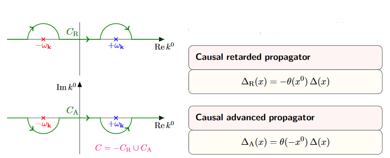
-
Apply Cauchy's integral formula to find in the case the sum of the residues at these two poles times , zero in the other case. (For the retarded propagator we get times the residues, because now the contours encircling non-trivial poles go clockwise).
-
The result is now non-singular at and therefore the limit is now computed by evaluating at .
This computation shows a) that the limiting distribution indeed exists, and b) that the support of is in the future, and that of is in the past.
Hence it only remains to see now that the support of is inside the causal cone. But this follows from the previous argument, by using that the Klein-Gordon equation is invariant under Lorentz transformations: This implies that the support is in fact in the future of every spacelike slice through the origin in , hence in the closed future cone of the origin.
Proposition
(causal propagator is skew-symmetric)
Under reversal of arguments the advanced and retarded causal propagators from prop. are related by
It follows that the causal propagator (95) is skew-symmetric in its arguments:
Proof
By prop. we have with (135)
Here in the second step we applied change of integration variables (which introduces no sign because in addition to the integration domain reverses orientation).
Proposition
(mode expansion of causal propagator for Klein-Gordon equation on Minkowski spacetime)
The causal propagator (95) for the Klein-Gordon equation for mass on Minkowski spacetime (example ) is given, in generalized function notation, by
where in the second line we used Euler's formula .
In particular this shows that the causal propagator is real, in that it is equal to its complex conjugate
Proof
By definition and using the expression from prop. for the advanced and retarded causal propagators we have
For the reality, notice from the last line that
where in the last step we used the change of integration variables (whih introduces no sign, since on top of the orientation of the integration domain changes).
We consider a couple of equivalent expressions for the causal propagator which are useful for computations:
Proposition
(causal propagator for Klein-Gordon operator on Minkowski spacetime as a contour integral)
The causal propagator (prop. ) for the Klein-Gordon equation at mass on Minkowski spacetime (example ) has the following equivalent expression, as a generalized function, given as a contour integral along a Jordan curve going counter-clockwise around the two poles at :
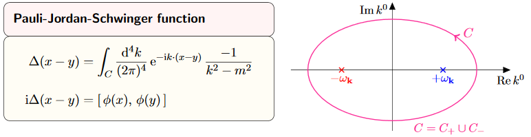
graphics grabbed from Kocic 16
Proof
By Cauchy's integral formula we compute as follows:
The last line is the expression for the causal propagator from prop.
Proposition
(causal propagator as Fourier transform of delta distribution on the Fourier transformed Klein-Gordon operator)
The causal propagator for the Klein-Gordon equation at mass on Minkowski spacetime has the following equivalent expression, as a generalized function:
where the integrand is the product of the sign function of with the delta distribution of the Fourier transform of the Klein-Gordon operator and a plane wave factor.
Proof
By decomposing the integral over into its negative and its positive half, and applying the change of integration variables we get
The last line is the expression for the causal propagator from prop. .
Prop. exhibits the causal propagator of the Klein-Gordon operator on Minkowski spacetime as the difference of a contribution for positive temporal angular frequency (hence positive energy and a contribution of negative temporal angular frequency.
The positive frequency contribution to the causal propagator is called the Wightman propagator (def. below), also known as the the vacuum state 2-point function of the free real scalar field on Minkowski spacetime. Notice that the temporal component of the wave vector is proportional to the negative angular frequency
(see at plane wave), therefore the appearance of the step function in (147) below:
Definition
(Wightman propagator or vacuum state 2-point function for Klein-Gordon operator on Minkowski spacetime)
The Wightman propagator for the Klein-Gordon operator at mass on Minkowski spacetime (example ) is the tempered distribution in two variables which as a generalized function is given by the expression
Here in the first line we have in the integrand the delta distribution of the Fourier transform of the Klein-Gordon operator times a plane wave and times the step function of the temporal component of the wave vector. In the second line we used the change of integration variables , then the definition of the delta distribution and the fact that is by definition the non-negative solution to the Klein-Gordon dispersion relation.
(e.g. Khavkine-Moretti 14, equation (38) and section 3.4)
Proposition
(Wightman propagator on Minkowski spacetime is distributional solution to Klein-Gordon equation)
The Wightman propagator (def. ) is a distributional solution (def. ) to the Klein-Gordon equation
Proof
By definition the Wightman propagator is the Fourier transform of distributions of the product of distributions
where in turn the argument of the delta distribution is just times the Fourier transform of the [Klein-Gordon operator]] itself (prop. ). This is clearly a solution to the equation
Under Fourier inversion (prop. ), this is the equation , as in the proof of prop. .
Proposition
(contour integral representation of the Wightman propagator for the Klein-Gordon operator on Minkowski spacetime)
The Wightman propagator from def. is equivalently given by the contour integral
where the Jordan curve runs counter-clockwise, enclosing the point , but not enclosing the point .
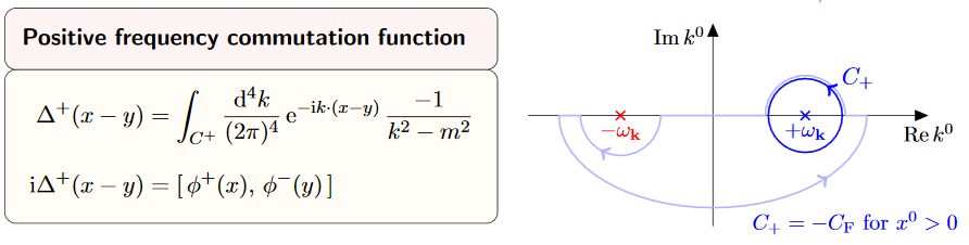
graphics grabbed from Kocic 16
Proof
We compute as follows:
The last step is application of Cauchy's integral formula, which says that the contour integral picks up the residue of the pole of the integrand at . The last line is , by definition .
Proposition
(skew-symmetric part of Wightman propagator is the causal propagator)
The Wightman propagator for the Klein-Gordon equation on Minkowski spacetime (def. ) is of the form
where
-
is the causal propagator (prop. ), which is real (146) and skew-symmetric (prop. )
-
is real and symmetric
(150)
Proof
By applying Euler's formula to (147) we obtain
On the left this identifies the causal propagator by (145), prop. .
The second summand changes, both under complex conjugation as well as under , via change of integration variables (because the cosine is an even function). This does not change the integral, and hence is symmetric.
We have seen that the positive frequency component of the causal propagator for the Klein-Gordon equation on Minkowski spacetime (prop. ) is the Wightman propagator (def. ) given, according to prop. , by (149)
There is an evident variant of this combination, which will be of interest:
Definition
(Feynman propagator for Klein-Gordon equation on Minkowski spacetime)
The Feynman propagator for the Klein-Gordon equation on Minkowski spacetime (example ) is the linear combination
where the first term is proportional to the sum of the advanced and retarded propagators (prop. ) and the second is the symmetric part of the Wightman propagator according to prop. .
Similarly the anti-Feynman propagator is
It follows immediately that:
Proposition
(Feynman propagator is symmetric)
The Feynman propagator and anti-Feynman propagator (def. ) are symmetric:
Proof
By equation (144) in cor. we have that is symmetric, and equation (150) in prop. says that is symmetric.
Proposition
(mode expansion for Feynman propagator of Klein-Gordon equation on Minkowski spacetime)
The Feynman propagator (def. ) for the Klein-Gordon equation on Minkowski spacetime is given by the following equivalent expressions
Similarly the anti-Feynman propagator is equivalently given by
Proof
By the mode expansion of from (135) and the mode expansion of from (151) we have
where in the second line we used Euler's formula. The last line follows by comparison with (147) and using that the integral over is invariant under .
The computation for is the same, only now with a minus sign in front of the cosine:
As before for the causal propagator, there are equivalent reformulations of the Feynman propagator which are useful for computations:
Proposition
(Feynman propagator as a Cauchy principal value)
The Feynman propagator and anti-Feynman propagator (def. ) for the Klein-Gordon equation on Minkowski spacetime is equivalently given by the following expressions, respectively:
where we have a limit of distributions as for the Cauchy principal value (this prop).
Proof
We compute as follows:
Here
-
In the first step we introduced the complex square root . For this to be compatible with the choice of non-negative square root for in (134) we need to choose that complex square root whose complex phase is one half that of (instead of that plus π). This means that is in the upper half plane and is in the lower half plane.
-
In the third step we observe that
-
for the integrand decays for positive imaginary part and hence the integration over may be deformed to a contour which encircles the pole in the upper half plane;
-
for the integrand decays for negative imaginary part and hence the integration over may be deformed to a contour which encircles the pole in the lower half plane
and then apply Cauchy's integral formula which picks out times the residue a these poles.
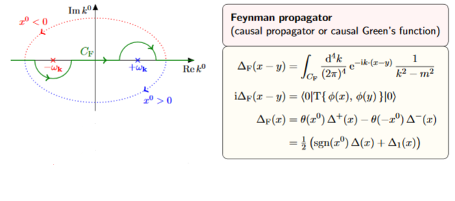
Notice that when completing to a contour in the lower half plane we pick up a minus signs from the fact that now the contour runs clockwise.
-
It follows that:
Proposition
(Feynman propagator is Green function)
The Feynman propagator for the Klein-Gordon equation on Minkowski spacetime (def. ) is proportional to a Green function for the Klein-Gordon equation in that
Proof
Equation (?) in prop. says that the Feynman propagator is the inverse Fourier transform of distributions of
This implies the statement as in the proof of prop. , via the analogue of equation (141).
singular support and wave front sets
We now discuss the singular support (def. ) and the wave front sets (def. ) of the various propagators for the Klein-Gordon equation on Minkowski spacetime.
Proposition
(singular support of the causal propagator of the Klein-Gordon equation on Minkowski spacetime is the light cone)
The singular support of the causal propagator for the Klein-Gordon equation on Minkowski spacetime, regarded via translation invariance as a generalized function in a single variable (136) is the light cone of the origin:
Proof
By prop. the causal propagator is equivalently the Fourier transform of distributions of the delta distribution of the mass shell times the sign function of the angular frequency; and by the basic properties of the Fourier transform (prop. ) this is the convolution of distributions of the separate Fourier transforms:
By prop. , the singular support of the first convolution factor is the light cone.
The second factor is
(by example and example ) and hence the wave front set (def. ) of the second factor is
With this the statement follows, via a partition of unity, from this prop..
For illustration we now make this general argument more explicit in the special case of spacetime dimension
by computing an explicit form for the causal propagator in terms of the delta distribution, the Heaviside distribution and smooth Bessel functions.
We follow (Scharf 95 (2.3.18)).
Consider the formula for the causal propagator in terms of the mode expansion (145). Since the integrand here depends on the wave vector only via its norm and the angle it makes with the given spacetime vector via
we may express the integration in terms of polar coordinates as follws:
In the special case of spacetime dimension this becomes
Here in the second but last step we renamed and doubled the integration domain for convenience, and in the last step we used the trigonometric identity .
In order to further evaluate this, we parameterize the remaining components of the wave vector by the dual rapidity , via
as
which makes use of the fact that is non-negative, by construction. This change of integration variables makes the integrals under the braces above become
Next we similarly parameterize the vector by its rapidity . That parameterization depends on whether is spacelike or not, and if not, whether it is future or past directed.
First, if is spacelike in that then we may parameterize as
which yields
where in the last line we observe that the integrand is a skew-symmetric function of .
Second, if is timelike with then we may parameterize as
which yields
Here in the last line we identified the integral representation of the Bessel function of order 0 (see here). The important point here is that this is a smooth function.
Similarly, if is timelike with then the same argument yields
In conclusion, the general form of is
Therefore we end up with
Proposition
(singular support of the Wightman propagator of the Klein-Gordon equation on Minkowski spacetime is the light cone)
The singular support of the Wightman propagator (def. ) for the Klein-Gordon equation on Minkowski spacetime, regarded via translation invariance as a distribution in a single variable, is the light cone of the origin:
Proof
By prop. the causal propagator is equivalently the Fourier transform of distributions of the delta distribution of the mass shell times the sign function of the angular frequency; and by basic properties of the Fourier transform (prop. ) this is the convolution of distributions of the separate Fourier transforms:
By prop. , the singular support of the first convolution factor is the light cone.
The second factor is
(by example and example and hence the wave front set (def. ) of the second factor is
With this the statement follows, via a partition of unity, from prop. .
For illustration, we now make this general statement fully explicit in the special case of spacetime dimension
by computing an explicit form for the causal propagator in terms of the delta distribution, the Heaviside distribution and smooth Bessel functions.
We follow (Scharf 95 (2.3.36)).
By (151) we have
The first summand, proportional to the causal propagator, which we computed as (155) in prop. to be
The second term is computed in a directly analogous fashion: The integrals from (153) are now
Parameterizing by rapidity, as in the proof of prop. , one finds that for timelike this is
while for spacelike it is
where we identified the integral representations of the Neumann function (see here) and of the modified Bessel function (see here).
As for the Bessel function in (154) the key point is that these are smooth functions. Hence we conclude that
This expression has singularities on the light cone due to the step functions. In fact the expression being differentiated is continuous at the light cone (Scharf 95 (2.3.34)), so that the singularity on the light cone is not a delta distribution singularity from the derivative of the step functions. Accordingly it does not cancel the singularity of as above, and hence the singular support of is still the whole light cone.
Proposition
(singular support of Feynman propagator for Klein-Gordon equation on Minkowski spacetime)
The singular support of the Feynman propagator and of the anti-Feynman propagator (def. ) for the Klein-Gordon equation on Minkowski spacetime, regarded via translation invariance as a distribution in a single variable, is the light cone of the origin:
(e.g DeWitt 03 (27.85))
Proof
By prop. the Feynman propagator is equivalently the Cauchy principal value of the inverse of the Fourier transformed Klein-Gordon operator:
Proposition
(wave front sets of propagators of Klein-Gordon equation on Minkowski spacetime)
The wave front set of the various propagators for the Klein-Gordon equation on Minkowski spacetime, regarded, via translation invariance, as distributions in a single variable, are as follows:
- the causal propagator (prop. ) has wave front set all pairs with and both on the lightcone:
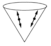
-
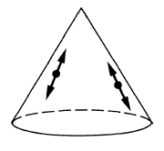
- the Wightman propagator (def. ) has wave front set all pairs with and both on the light cone and :
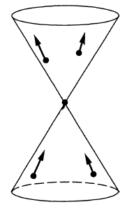
- the Feynman propagator (def. ) has wave front set all pairs with and both on the light cone and
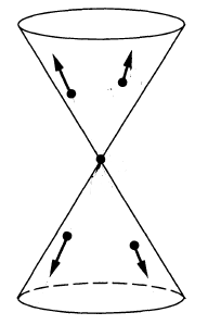
Proof
First regarding the causal propagator:
By prop. the singular support of is the light cone.
Since the causal propagator is a solution to the homogeneous Klein-Gordon equation, the propagation of singularities theorem (prop. ) says that also all wave vectors in the wave front set are lightlike. Hence it just remains to show that all non-vanishing lightlike wave vectors based on the lightcone in spacetime indeed do appear in the wave front set.
To that end, let be a bump function whose compact support includes the origin.
For a point on the light cone, we need to determine the decay property of the Fourier transform of . This is the convolution of distributions of with . By prop. we have
This means that the convolution product is the smearing of the mass shell by .
Since the mass shell asymptotes to the light cone, and since for on the light cone (given that is on the light cone), this implies the claim.
Now for the Wightman propagator:
By def. its Fourier transform is of the form
Moreover, its singular support is also the light cone (prop. ).
Therefore now same argument as before says that the wave front set consists of wave vectors on the light cone, but now due to the step function factor it must satisfy .
Finally regarding the Feynman propagator:
by prop. the Feynman propagator coincides with the positive frequency Wightman propagator for and with the “negative frequency Hadamard operator” for . Therefore the form of now follows directly with that of above.
propagators for the Dirac equation on Minkowski spacetime
We now discuss how the propagators for the free Dirac field on Minkowski spacetime (example ) follow directly from those for the scalar field discussed above.
Proposition
(advanced and retarded propagator for Dirac equation on Minkowski spacetime)
Consider the Dirac operator on Minkowski spacetime, which in Feynman slash notation reads
Its advanced and retarded propagators (def. ) are the derivatives of distributions of the advanced and retarded propagators for the Klein-Gordon equation (prop. ) by :
Hence the same is true for the causal propagator:
Proof
Applying a differential operator does not change the support of a smooth function, hence also not the support of a distribution. Therefore the uniqueness of the advanced and retarded propagators (prop. ) together with the translation-invariance and the anti-formally self-adjointness of the Dirac operator (as for the Klein-Gordon operator (136) implies that it is sufficent to check that applying the Dirac operator to the yields the delta distribution. This follows since the Dirac operator squares to the Klein-Gordon operator:
Similarly we obtain the other propagators for the Dirac field from those of the real scalar field:
Definition
(Wightman propagator for Dirac operator on Minkowski spacetime)
The Wightman propagator for the Dirac operator on Minkowski spacetime is the positive frequency part of the causal propagator (prop. ), hence the derivative of distributions (def. ) of the Wightman propagator for the Klein-Gordon field (def. ) by the Dirac operator:
Here we used the expression (?) for the Wightman propagator of the Klein-Gordon equation.
Definition
(Feynman propagator for Dirac operator on Minkowski spacetime)
The Feynman propagator for the Dirac operator on Minkowski spacetime is the linear combination
of the Wightman propagator (def. ) and the retarded propagator (prop. ). By prop. this means that it is the derivative of distributions (def. ) of the Feynman propagator of the Klein-Gordon equation (def. ) by the Dirac operator
This concludes our discussion of propagators induced from the covariant phase space of Green hyperbolic free Lagrangian field theory. These propagators will be the key in for quantization via causal perturbation theory. But not all free field theories have a covariant phase space of Green hyperbolic equations of motion, for instance the electromagnetic field, a priori, does not. Therefore before turning to quantization in the next chapter we first discuss how gauge symmetries obstruct the existence of Green hyperbolic equations of motion.
Gauge symmetries
In this chapter we discuss these topics:
An infinitesimal gauge symmetry of a Lagrangian field theory (def. below) is a infinitesimal symmetry of the Lagrangian which may be freely parameterized, hence “gauged”, by a gauge parameter. A Lagrangian field theory exhibiting these is also called a gauge theory.
By choosing the gauge parameter to have compact support, infinitesimal gauge symmetries in particular yield infinitesimal symmetries of the Lagrangian with compact spacetime support. One finds (prop. below) that the existence of on-shell non-trivial symmetries of this form is an obstruction to the existence of the covariant phase space of the theory (prop. ).
| name | meaning | def. |
|---|---|---|
| infinitesimal symmetry of the Lagrangian | evolutionary vector field which leaves invariant the Lagrangian density up to a total spacetime derivative | def. |
| spacetime-compactly supported infinitesimal symmetry of the Lagrangian | obstructs existence of the covariant phase space (if non-trivial on-shell) | prop. |
| infinitesimal gauge symmetry | gauge parameterized collection of infinitesimal symmetries of the Lagrangian; for compactly supported gauge parameter this yields spacetime-compactly supported infinitesimal symmetries | def. |
| rigid infinitesimal symmetry of the Lagrangian | infinitesimal symmetry modulo gauge symmetry | def. |
| generating set of gauge parameters | reflects all the Noether identities | remark |
| closed gauge parameters | Lie bracket of infinitesimal gauge symmetries closes on gauge parameters | def. |
But we may hard-wire these gauge equivalences into the very geometry of the types of fields by forming the homotopy quotient of the action of the infinitesimal gauge symmetries on the jet bundle. This homotopy quotient is modeled by the action Lie algebroid (def. below). Its algebra of functions is the local BRST complex of the theory (def. ) below.
In this construction the gauge parameters appear as auxiliary fields whose field bundle is a graded version of the gauge parameter-bundle. As such they are called ghost fields. The ghost fields may have infinitesimal gauge symmetries themselves which leads to ghost-of-ghost fields, etc. (example ) below.
It is these auxiliary ghost fields and ghost-of-ghost fields which will serve to remove the obstruction to the existence of the covariant phase space for gauge theories, this we arrive at in Gauge fixing, further below.
gauge parameters and ghost fields
| symbol | meaning | def. |
|---|---|---|
| gauge parameter bundle | def. | |
| coordinate function on gauge parameter bundle | ||
| gauge parameter | ||
| gauge parameter bundle regarded as graded manifold in degree 1 | expl. | |
| gost field history | ||
| ghost field component function | ||
| ghost field jet component function | ||
| gauge-of-gauge parameter bundle | expl. | |
| coordinate function on gauge-of-gauge parameter bundle | ||
| gauge-of-gauge parameter | ||
| gauge-of-gauge parameter bundle regarded as graded manifold in degree 1 | ||
| gost-of-ghost field history | ||
| ghost-of-ghost field component function | ||
| ghost-of-ghost field jet component function |
The mathematical theory capturing these phenomena is the higher Lie theory of Lie-∞ algebroids (def. below).
compactly supported infinitesimal symmetries obstruc the covariant phase space
As an immediate corollary of prop. we have the following important observation:
Proposition
(spacetime-compactly supported and on-shell non-trivial infinitesimal symmetries of the Lagrangian obstruct the covariant phase space)
Let be a Lagrangian field theory over a Lorentzian spacetime.
If there exists a single infinitesimal symmetry of the Lagrangian (def. ) such that
then there does not exist any Cauchy surface (def. ) for the Euler-Lagrange equations of motion (def. ) outside the spacetime support of .
Proof
By prop. the flow along preserves the on-shell space of field histories. Now by the assumption that does not vanish on-shell implies that this flow is non-trivial, hence that it does continuously change the field histories over some points of spacetime, while the assumption that it has compact spacetime support means that these changes are confined to a compact subset of spacetime.
This means that there is a continuum of solutions to the equations of motion whose restriction to the infinitesimal neighbourhood of any codimension-1 suface outside of this compact support coincides. Therefore this restriction map is not an isomorphism and not a Cauchy surface for the equations of motion.
Notice that there always exist spacetime-compactly supported infinitesimal symmetries that however do vanish on-shell:
Example
(trivial compactly-supported infinitesimal symmetries of the Lagrangian)
Let be a Lagrangian field theory (def. ) over Minkowski spacetime (def. ), so that the Lagrangian density is canonically of the form
with Lagrangian function a smooth function of the jet bundle (characterized by prop. ).
Then every evolutionary vector field (def. ) whose coefficients which is proportional to the Euler-Lagrange derivative (50) of the Lagrangian function
by smooth coefficient functions
such that
is an implicit infinitesimal gauge symmetry (def. ).
This is so for a “trivial reason” namely due to that that skew symmetry:
Here the first steps are just recalling those in the proof of Noether's theorem I (prop. ) while the last step follows with the skew-symmetry of .
Notice that this means that
-
the Noether current (79) vanishes: ;
Therefore these implicit infinitesimal gauge symmetries are called the trivial infinitesimal gauge transformations.
(e.g. Henneaux 90, section 2.5)
Proposition implies that we need a good handle on determining whether the space of non-trivial compactly supported infinitesimal symmetries of the Lagrangian modulo trivial ones is non-zero. This obstruction turns out to be neatly captured by methods of homological algebra applied to the local BV-complex (def. ):
Example
(cochain cohomology of local BV-complex)
Let be a Lagrangian field theory (def. ) whose field bundle is a trivial vector bundle (example ) and whose Lagrangian density is spacetime-independent (example ), and let be a constant section of the shell (59).
By inspection we find that the cochain cohomology of the local BV-complex (def. ) has the following interpretation:
In degree 0 the image of the BV-differential coming from degree -1 and modulo -exact terms
is the ideal of functions modulo that vanish on-shell. Since the differential going from degree 0 to degree 1 vanishes, the cochain cohomology in this degree is the quotient ring
of functions on the shell (109).
In degree -1 the kernel of the BV-differential going to degree 0
is the space of implicit infinitesimal gauge symmetries (def. ) and the image of the differential coming from degree -2
is the trivial implicit infinitesimal gauge transformations (example ).
Therefore the cochain cohomology in degree -1 is the quotient space of implicit infinitesimal gauge transformations modulo the trivial ones:
Proposition
(local BV-complex is homological resolution of the shell iff there are no non-trivial compactly supported infinitesimal symmetries)
Let be a Lagrangian field theory (def. ) whose field bundle is a trivial vector bundle (example ) and whose Lagrangian density is spacetime-independent (example ) and let be a constant section of the shell (59). Furthermore assume that is at least quadratic in the vertical coordinates around .
Then the local BV-complex of local observables (def. ) is a homological resolution of the algebra of functions on the infinitesimal neighbourhood of in the shell (example ), hence the canonical comparison morphisms (113) is a quasi-isomorphism precisely if there is no non-trivial (example ) implicit infinitesimal gauge symmetry (def. ):
Proof
By example the vanishing of compactly supported infinitesimal symmetries is equivalent to the vanishing of the cochain cohomology of the local BV-complex in degree -1 (156).
Therefore the statement to be proven is equivalently that the Koszul complex of the sequence of elements
is a homological resolution of , hence has vanishing cohomology in all negative degrees, already if it has vanishing cohomology in degree -1.
By a standard fact about Koszul complexes (this prop.) a sufficient condition for this to be the case is that
-
the ring is the tensor product of with a Noetherian ring;
-
the elements are contained in its Jacobson radical.
The first condition is the case since is by definition a formal power series ring over a field tensored with (by this example). Since the Jacobson radical of a power series algebra consists of those elements whose constant term vanishes (see this example), the assumption that is at least quadratic, hence that is at least linear in the fields, guarantees that all are contained in the Jacobson radical.
Prop. says what gauge fixing has to accomplish: given a local BV-BRST complex we need to find a quasi-isomorphism to another complex which is such that it comes from a graded Lagrangian density whose BV-cohomology vanishes in degree -1 and hence induces a graded covariant phase space, and such that the remaining BRST differential respects the Poisson bracket on this graded covariant phase space.
infinitesimal gauge symmetries
Prop. says that the problem is to identify the presence of spacetime-compactly supported infinitesimal symmetries that are on-shell non-trivial. One way they may be identified is if infinitesimal symmetries appear in linearly parameterized collections, where the parameter itself is an arbitrary spacetime-dependent section of some fiber bundle (hence is itself like a field history), because then choosing the parameter to have compact support yields an infinitesimal symmetry of the Lagrangian with compact spacetime support (remark below).
In this case we speak of a gauge parameter (def. below). It turns out that in most examples of Lagrangian field theories of interest, the compactly supported infinitesimal symmetries all come from gauge parameters this way. Therefore we now consider this case in detail.
Definition
(infinitesimal gauge symmetries)
Let be a Lagrangian field theory (def. ).
Then a collection of infinitesimal gauge symmetries of is
-
a vector bundle over spacetime of positive rank, to be called a gauge parameter bundle;
-
a bundle morphism (def. ) from the jet bundle of the fiber product with the field bundle (def. ) to the vertical tangent bundle of (def. ):
such that
-
is linear in the first argument (in the gauge parameter);
-
is an evolutionary vector field on (def. );
-
is an infinitesimal symmetry of the Lagrangian (def. ) in the second argument.
We may express this equivalently in components in the case that the field bundle is a trivial vector bundle with field fiber coordinates (example ) and also happens to be a trivial vector bundle
where is a vector space with coordinate functions .
Then may be expanded in the form
where the components
are smooth functions on the jet bundle of , locally of finite order (prop. ), and such that the Lie derivative of the Lagrangian density along is a total spacetime derivative, which by Noether's theorem I (prop. ) means in components that
(e.g. Henneaux 90 (3))
The point is that infinitesimal gauge symmetries in particular yield spacetime-compactly supported infinitesimal gauge symmetries as in prop. :
Remark
(infinitesimal gauge symmetries yield spacetime-compactly supported infinitesimal symmetries of the Lagrangian)
Let be a Lagrangian field theory (def. ) and a bundle of gauge parameters for it (def. ) with gauge parametrization
Then for every smooth section of the gauge parameter bundle (def. ) there is an induced infinitesimal symmetry of the Lagrangian (def. ) given by the composition of with the jet prolongation of (def. )
In terms of the components (157) this means that
where now
are the actual spacetime partial derivatives of the gauge parameter section (which are functions of spacetime).
In particular, since is assumed to be a vector bundle, there always exists gauge parameter sections that have compact support (bump functions). For such compactly supported the infinitesimal symmetry is spacetime-compactly supported as in prop. .
The following remark and def. introduce some useful terminology:
Remark
(generating set of gauge transformations)
Given a Lagrangian field theory, then a choice of gauge parameter bundle with gauge parameterized infinitesimal gauge symmetries (def. ) is indeed a choice and not uniquely fixed.
For example given any such bundle one may form the direct sum of vector bundles with any other smooth vector bundle over , extend by zero to , and thereby obtain another gauge parameterized of infinitesimal gauge symmetries
Conversely, given any subbundle , then the restriction of to is still a gauge parameterized collection of infinitesimal gauge symmetries.
We will see that for the purpose of removing the obstruction to the existence of the covariant phase space, the gauge parameters have to capture all Noether identities (prop. ). In this case one says that the gauge parameter bundle is a generating set.
(e.g. Henneaux 90, section (2.8))
Definition
(rigid infinitesimal symmetries of the Lagrangian)
Let be a Lagrangian field theory (def. ) and let be infinitesimal gauge symmetries (def. ) whose gauge parameters form a generating set (remark ).
Then the vector space of rigid infinitesimal symmetries of the Lagrangian is the quotient space of the infinitesimal symmetries of the Lagrangian by the image of the infinitesimal gauge symmetries:
The following is a way to identify infinitesimal gauge symmetries:
Proposition
(Noether's theorem II – Noether identities)
Let be a Lagrangian field theory (def. ) and let be a vector bundle.
Then a bundle morphism of the form
is a collection of infinitesimal gauge symmetries (def. ) with local components (157)
precisely if the Euler-Lagrange form (prop. ) satisfies the following conditions:
These relations are called the Noether identities of the Euler-Lagrange equations of motion (def ).
Proof
By Noether's theorem I, is an infinitesimal symmetry of the Lagrangian precisely if the contraction (def. ) of with the Euler-Lagrange form (prop. ) is horizontally exact:
From (157) this means that
where in the last step we used jet-level integration by parts (example ) to move the total spacetime derivatives off of , thereby picking up some horizontally exact correction term, as shown.
This means that the term over the brace is horizontally exact:
But now the term on the left is independent of the jet coordinates of positive order , while the horizontal derivative increases the dependency on the jet order by one. Therefore the term on the left is horizontally exact precisely if it vanishes, which is the case precisely if the coefficients of vanish, which is the statement of the Noether identities.
Alternatively we may reach this conclusion from (159) by applying to both sides of (159) the Euler-Lagrange derivative (50) with respect to . On the left this yields again the coefficients of , while by the argument from example it makes the right hand side vanish.
As a corollary we obtain:
Proposition
(conserved charge of infinitesimal gauge symmetry vanishes)
The conserved current (def. )
which corresponds to an infinitesimal gauge symmetry (def. ) by Noether's first theorem (prop. ), is up to a term which vanishes on-shell (52)
not just on-shell-conserved, but off-shell-conserved, in that its total spacetime derivative vanishes identically:
Moreover, if the field bundle as well as the gauge parameter-bundles are trivial vector bundles over Minkowski spacetime (example ) then is horizontally exact on-shell (52)
In particular the conserved charge (prop. )
corresponding to an infinitesimal gauge symmetry vanishes on every codimension one submanifold of spacetime (without boundary, ):
Proof
Take to be as in equation (158):
By the construction there, manifestly vanishes on the prolonged shell (52), being a sum of total spacetime derivatives of terms proportional to the components of the Euler-Lagrange form.
By Noether's second theorem (prop. ) we have and hence
Now if the field bundle and gauge parameter bundle are trivial, then prop. implies that
By restricting this equation to the prolonged shell and using that , it follows that .
This implies by prop. and Stokes' theorem (prop. ).
This situation has a concise cohomological incarnation:
Example
(Noether's theorems I and II in terms of local BV-cohomology)
Let be a Lagrangian field theory (def. ) over Minkowski spacetime of dimension , and let be a gauge parameter bundle (def. ) which is closed (def. ). Assume that both are trivial vector bundles (example ) with field coordinates as in prop. .
Then in the local BV-complex (def. ) we have:
The -closure of an element in total degree is characterizes as the direct sum of an evolutionary vector field which is an infinitesimal symmetry of the Lagrangian and theconserved current that corresponds to it under Noether's first theorem (prop. ).
Moreover, such a pair is -exact precisely if the infinitesimal symmetry of the Lagrangian is in fact an infinitesimal gauge symmetry as witnessed by Noether's second theorem (prop. ).
(Barnich-Brandt-Henneaux 94, top of p. 20)
Proof
An element of the local BV-complex in degee is the direct sum of a horizontal differential form of degree with the product of a horizontal form of degree times a function proportional to the antifields:
Its closure means that
where the equality in the top right corner is euqation
It being exact means that
where now the equality in the second term from the left is equation (160) for conserved currents corresponding to infinitesimal gauge symmetries (prop. ).
We will need some further technical results on Noether identities:
Definition
Let be a Lagrangian field theory (def. ) over Minkowski spacetime of dimension , and let be a gauge parameter bundle (def. ) which is closed (def. ). Assume that both are trivial vector bundles (example ) with field coordinates as in prop. .
A Noether operator is a differential operator (def. ) from the vertical cotangent bundle of (example ) to the trivial real line bundle
such that it annihilates the Euler-Lagrange form (prop. ):
Given For an evolutionary vector field which is an infinitesimal symmetry of the Lagrangian (def. ), we define a new differentia opeator by
where denotes the prolongation of the evolutionary vector field (prop. ) and where denotes the formally adjoint differential operator (def. ) of the evolutionary derivative of (def. ).
Proposition
(Lie algebra action of infinitesimal symmetries of the Lagrangian on Noether operators)
The operation (161) exhibits a Lie algebra action of the Lie algebra of infinitesimal symmetries of the Lagrangian (prop. ) on Noether operators (def. ), in that
-
is again a Noether operator;
-
.
Moreover, if denotes the map which identifies a Noether identity with an infinitesimal gauge symmetry by Noether's second theorem (def. ) then
where on the right we have again the Lie bracket of evolutionary vector fields from (prop. ).
(Barnich 10, prop. 3.1 and (3.8))
Proof
For the first statement observe that by the product law for differentiation we have
where on the right we used (82).
Here are examples of infinitesimal gauge symmetries in Lagrangian field theory:
Example
(infinitesimal gauge symmetry of electromagnetic field)
Consider the Lagrangian field theory of free electromagnetism on Minkowski spacetime from example . With field coordinates denoted the Lagrangian density is
where is the universal Faraday tensor from example .
Let be the trivial line bundle, regarded as a gauge parameter bundle (def. ) with coordinate functions .
Then a gauge parametrized evolutionary vector field (157) is given by
This is because already the universal Faraday tensor is invariant under this flow:
because partial derivatives commute with each other: (29).
Equivalently, the Euler-Lagrange form
of the theory (example ), corresponding to the vacuum Maxwell equations (example ), satisfies the following Noether identity (prop. ):
again due to the fact that partial derivatives commute with each other.
This is the archetypical infinitesimal gauge symmetry that gives gauge theory its name.
More generally:
Example
(infinitesimal gauge symmetry of Yang-Mills theory)
For a semisimple Lie algebra, consider the Lagrangian field theory of Yang-Mills theory on Minkowski spacetime from example , with Lagrangian density
given by the universal field strength (31)
Let be the trivial vector bundle with fiber , regarded as a gauge parameter bundle (def. ) with coordinate functions .
Then a gauge parametrized evolutionary vector field (157) is given by
We compute the derivative of the Lagrangian function along this vector field:
Here in the third step we used that (29), so that its contraction with the skew-symmetric vanishes, and in the last step we used that for a semisimple Lie algebra is totally skew symmetric.
So the Lagrangian density of Yang-Mills theory is strictly invariant under these infinitesimal gauge symmetries.
Example
(infinitesimal gauge symmetry of the B-field)
Consider the Lagrangian field theory of the B-field on Minkowski spacetime from example , with field bundle the differential 2-form-bundle with coordinates subject to ; and with Lagrangian density
for
the universal B-field strength (example ).
Let be the cotangent bundle (def. ), regarded as a gauge parameter bundle (def. ) with coordinate functions as in example .
Then a gauge parametrized evolutionary vector field (157) is given by
In fact this leaves the Lagrangian function invariant, in direct higher analogy to example :
due to the symmetry of partial derivatives (29).
While so far all this is in direct analogy to the case of the electromagnetic field (example ), just with field histories being differential 1-forms now replaced by differential 2-forms, a key difference is that now the gauge parameterization itself has infinitesimal gauge symmetries:
Let
be the trivial real line bundle with coordinates , to be regarded as a second order infinitesimal gauge-of-gauge symmetry, then
with prolongation
has the property that
We further discuss these higher gauge transformations below.
Lie algebra actions and Lie algebroids
We have seen above infinitesimal gauge symmetries implied by a Lagrangian field theory, exhibited by infinitesimal symmetries of the Lagrangian. In order to remove the obstructions that these infinitesimal gauge symmetries cause for the existence of the covariant phase space (via prop. and remark ) we will need (discussed below in Gauge fixing) to make these symmetries manifest by hard-wiring them into the geometry of the type of fields. Mathematically this means that we need to take the homotopy quotient of the jet bundle of the field bundle by the action of the infinitesimal gauge symmetries, which is modeled by their action Lie algebroid.
Here we introduce the required higher Lie theory of Lie ∞-algebroids (def. below). Further below we specify this to actions by infinitesimal gauge symmetries to obtain the local BRST complex of a Lagrangian field theory (def. ) below.
The following discussion introduces and uses the tremendously useful fact that (higher) Lie theory may usefully be dually expressed in terms of differential graded-commutative algebra (def. below), namely in terms of “Chevalley-Eilenberg algebras”. In the physics literature, besides the BRST-BV formalism, this fact underlies the D'Auria-Fré formulation of supergravity (“FDAs”, see the convoluted history of the concept). Mathematically the deep underlying phenomenon is called the “Koszul duality between the Lie operad and the commutative algebra operad”, but this need not concern us here. The phenomenon is readily seen in direct application:
Before we proceed, we make explicit a structure wich we already encountered in example .
Definition
(differential graded-commutative superalgebra)
A differential graded-commutative superalgebra is
-
a cochain complex of super vector spaces, hence for each
1 a super vector space ;
-
a super-degree preserving linear map
such that
-
1, an associative algebra-structure on
such that for all with homogenous bidegree we have the super sign rule
-
.
A homomorphism between two differential graded-commutative superalgebras is a linear map between the underlying super vector spaces which preserves both degrees, and respects the product as well as the differential .
We write for the category of differential graded-commutative superalgebra.
For the super sigsn rule appearing here see also e.g. Castellani-D’Auria-Fré 91 (II.2.106) and (II.2.109), Deligne-Freed 99, section 6.
Example
(de Rham algebra of super differential forms is differential graded-commutative superalgebra)
For a super Cartesian space, def. (or more generally a supermanifold, def. ) the de Rham algebra of super differential forms from def.
is a differential graded-commutative superalgebra (def. ) with product the wedge product of differential forms and differential the de Rham differential.
We will recognize the dual incarnation of this in higher Lie theory below in example .
Proposition
(Lie algebra in terms of Chevalley-Eilenberg algebra)
Let be a finite dimensional super vector space equipped with a super Lie bracket . Write for the dual vector space and for the linear dual map of the Lie bracket. Then on the Grassmann algebra (which is -bigraded as in def. ) the graded derivation of degree , which on is given by constitutes a differential in that . The resulting differential graded-commutative algebra is called the Chevalley-Eilenberg algebra
In components:
If is a linear basis of , so that the Lie bracket is given by the structure constants as
and if denotes the corresponding dual basis, then is equivalently the differential graded-commutative superalgebra (def. ) generated from the in bi-degree , where is the super-degree of as in def. subject to the relation
and the differential is given by
Notice that by degree-reasons every degree +1 derivation on is of this form,
The condition that is equivalently the (super-)Jacobi identity on the bracket , making it an actual (super-)Lie bracket:
(where the square brackets on the right denote super-skew-symmetrization).
Hence not only is a differential graded-commutative superalgebra (def. ) whenever is a super Lie algebra, but conversely super Lie algebra-structure on a super vector space is the same as a differential of degree on the Grassmann algebra .
We may state this equivalence in a more refined form: A homomorphism between super vector space is, by degree-reasons, the same as a graded algebra homomorphism and it is immediate to check that is a homomorphism of super Lie algebras precisely if is a homomorpism of differential algebras:
This is a natural bijection between homomrophism of super Lie algebras and of differential graded-commutative superalgebras (def. )
Stated more abstractly this means that forming Chevalley-Eilenberg algebras is a fully faithful functor
Notice that prop. establishes a dual algebraic incarnation of (super-)Lie algebras which is of analogous form as the dual algebraic characterization of (super-)Cartesian spaces from prop. and def. . In fact both these concepts unify into the concept of an action Lie algebroid:
Definition
(action of Lie algebra by infinitesimal diffeomorphism)
Let be a supermanifold (def. ), for instance a super Cartesian space (def. ), and let be a finite dimensional super Lie algebra as in prop. .
An action of on by infinitesimal diffeomorphisms, is a homomorphism of super Lie algebras
to the tangent vector fields on (example )
Equivalently – to bring out the relation to the gauge parameterized infinitesimal gauge transformations in def. – this is a -parameterized section
of the tangent bundle, such that for all pairs of points in we have
(with the Lie bracket of tangent vector fields on the left).
In components:
If is a linear basis of with corresponding structure constants (as in prop. ) and if is a coordinate chart of , then is given by
Now the construction of the Chevalley-Eilenberg algebra of a super Lie algebra (prop. ) extends to the case where this super Lie algebra acts on a supermanifold (def. ):
Definition
Given a Lie algebra action
of a finite-dimensional super Lie algebra on a supermanifold (def. ) we obtain a differential graded-commutative superalgebra to be denoted
-
whose underlying graded-commutative superalgebra is the Grassmann algebra of the -free module on over
which means that the graded manifold underlying the action Lie algebroid according to remark is
(170) -
whose differential is given
- on functions by the linear dual of the Lie algebra action
-
on dual Lie algebra elements by the linear dual of the Lie bracket
In components:
Assume that is a super Cartesian space with coordinate functions and let be a linear basis for with dual basis for and structure constants as in prop. and with the Lie action given in components as in def. . Then the differential is given by
We may summarize this by writing the derivation as follows:
That this squares to zero is equivalently
-
in degree 0 the action property:
-
in degree 1 the Jacobi identity (169).
Hence as before in prop. the Lie theoretic structure is faithfully captured dually by differential graded-commutative superalgebra.
We call the formal dual of this dgc-superalgebra the action Lie algebroid of acting on .
The concept emerging by this example we may consider generally:
Definition
Let be a supermanifold (def. ) (for instance a super Cartesian space, def. ) and write for its algebra of functions. Then a connected super Lie ∞-algebroid over of finite type is a
-
a sequence of free modules of finite rank over , hence a graded module in degrees ;
-
a differential that makes the graded-commutative algebra into a cochain differential graded-commutative algebra (hence with of degree +1) over (not necessarily over ), to be called the Chevalley-Eilenberg algebra of :
(172)
If we allow to also have terms in non-positive degree, then we speak of a derived Lie algebroid. If is only concentrated in negative degrees, we also speak of a derived manifold.
With canonically itself regarded as a differential graded-commutative superalgebra, there is a canonical dg-algebra homomorphism
which is the identity on and zero on .
(We discuss homomorphism between Lie ∞-algebroid below in def. .)
Remark
(Lie algebroids as differential graded manifolds)
Definition of derived Lie algebroids is an encoding in higher algebra (homological algebra, in this case) of a situation that is usefully thought of in terms of higher differential geometry.
To see this, recall the magic algebraic properties of ordinary differential geometry (prop. )
-
embedding of smooth manifolds into formal duals of R-algebras;
-
embedding of smooth vector bundles into formal duals of modules
Together these imply that we may think of the graded algebra underlying a Chevalley-Eilenberg algebra as being the algebra of functions on a graded manifold
which is infinitesimal in non-vanishing degree.
The “higher” in higher differential geometry refers to the degrees higher than zero. See at Higher Structures for exposition. Specifically if has components in negative degrees, these are also called derived manifolds.
Example
(basic examples of Lie algebroids)
Two basic examples of Lie algebroids are:
-
For any supermanifold (def. ), for instance a super Cartesian space (def. ) then setting and makes it a Lie algebroid in the sense of def. .
-
For a finite-dimensional super Lie algebra, its Chevalley-Eilenberg algebra (prop. ) exhibits as a Lie algebroid in the sense of def. . We write or for regarded as a Lie algebroid this way.
-
For and as in the previous items, and for a Lie algebra action (def. ) of on , then the dgs-superalegbra from def. defines a Lie algebroid in the sense of def. , the action Lie algebroid.
In the special case that this reduces to the first example, while for this reduces to the second example.
Here is another basic examples of Lie algebroids that will plays a role:
Example
(horizontal tangent Lie algebroid)
Let be a smooth manifold or more generally a supermanifold or more generally a locally pro-manifold (prop. ). Then we write for the Lie algebroid over and whose Chevalley-Eilenberg algebra is generated over in degree 1 from the module
of differential 1-forms and whose Chevalley-Eilenberg differential is the de Rham differential, so that the Chevalley-Eilenberg algebra is the de Rham dg-algebra of super differential forms (example )
This is called the tangent Lie algebroid of . As a graded manifold (via remark ) this is called the “shifted tangent bundle” of .
More generally, let be a fiber bundle over . Then there is a Lie algebroid over the jet bundle of (def. ) defined by its Chevalley-Eilenberg algebra being the horizontal part of the variational bicomplex (def. ):
The underlying graded manifold of is the fiber product of the jet bundle of with the shifted tangent bundle of .
There is then a canonical homomorphism of Lie algebroids (def. )
With the general concept of Lie algebra action (def. ) and the corresponding action Lie algebroids (def. ) and more general Lie ∞-algebroids in hand (def. ) we now apply this to the action of infinitesimal gauge symmetries (def. ) on field histories of a Lagrangian field theory, but we consider this locally, namely on the jet bundle. The Chevalley-Eilenberg algebra of the resulting action Lie algebroid (def. ) is known as the local BRST complex, example below.
The Lie algebroid-perspective on BV-BRST formalism has been made explicit in (Barnich 10).
Definition
(closed gauge parameters)
Let be a Lagrangian field theory (def. ). Then a gauge parameter bundle parameterizing infinitesimal gauge symmetries (def. )
is called closed if it is closed under the Lie bracket of evolutionary vector fields (prop. ) in that there exists a morphism (not necessarily uniquely)
such that
where on the left we have the Lie bracket of evolutionary vector fields from prop. .
Beware that may be a function of the fields, namely of the jet bundle of the field bundle . Hence for closed gauge parameters in general defines a Lie algebroid-structure (def. ).
Notice that the collection of all infinitesimal symmetries of the Lagrangian by necessity always forms a (very large) Lie algebra. The condition of closed gauge parameters is a condition on the choice of parameterization of the infinitesimal gauge symmetries, see remark .
Recall the general concept of a Lie algebra action from def. . The following realizes this for the action of closed infinitesimal gauge symmetries on the jet bundle of a Lagrangian field theory.
Example
(action of closed infinitesimal gauge symmetries on fields)
Let be a Lagrangian field theory (def. ), and let be a bundle of gauge parameters (def. ) paramaterizing infinitesimal gauge symmetries
which are closed (def. ), via a bracket .
By passing from these evolutionary vector fields (def. ) to their prolongations , being actual vector fields on the jet bundle (prop. ), we obtain a bundle morphism of the form
and via the assumed bracket on gauge parameters this exhibits Lie algebroid structure on .
In the case that is a trivial vector bundle, with fiber , then so is its jet bundle
If moreover the bracket (173) on the infinitesimal gauge symmetries is independent of the fields, then this induces a Lie algebra structure on and exhibits an Lie algebra action
of the gauge parameterized infinitesimal gauge symmetries on the jet bundle of the field bundle by infinitesimal diffeomorphisms.
Example
(local BRST complex and ghost fields for closed infinitesimal gauge symmetries)
Let be a Lagrangian field theory (def. ), and let be a bundle of irreducible closed gauge parameters for the theory (def. ) with bundle morphism
Assuming that the gauge parameter bundle is trivial, , then by example this induces an action of a Lie algebra on by infinitesimal diffeomorphisms.
The corresponding action Lie algebroid (def. ) has as underlying graded manifold (remark )
the jet bundle of the graded field bundle
which regards the gauge parameters as fields in degree 1. As such these are called ghost fields:
Therefore we write suggestively
for the action Lie algebroid of the gauge parameterized implicit infinitesimal gauge symmetries on the jet bundle of the field bundle.
The Chevalley-Eilenberg differential of the BRST complex is traditionally denoted
To express this in coordinates, assume that the field bundle as well as the gauge parameter bundle are trivial vector bundles (example ) with the field coordinates on the fiber of with induced jet coordinates and are ghost field coordinates on the fiber of with induced jet coordinates .
Then in terms of the corresponding coordinate expression for the gauge symmetries (157) the BRST differential is given on the fields by
and on the ghost fields by
and it extends from there, via prop. , to jets of fields and ghost fields by (anti-)commutativity with the total spacetime derivative.
Moreover, since the action of the infinitesimal gauge symmetries is by definition via prolongations (prop. ) of evolutionary vector fields (def. ) and hence compatible with the total spacetime derivative (75) this construction descends to the horizontal tangent Lie algebroid (example ) to yield
The Chevalley-Eilenberg differential on is
The Chevalley-Eilenberg algebra of functions on this differential graded manifold (172) is called the off-shell local BRST complex.
(Barnich-Brandt-Henneaux 94, Barnich 10 (35)).
Definition
(global BRST complex)
We may pass from the off-shell local BRST complex (def. ) on the jet bundle to the “global” BRST complex by transgression of variational differential forms (def. ):
Write for the induced graded off-shell algebra of observables (def. ). For with corresponding local observable its BRST differential is defined by
and extended from there to as a graded derivation.
Examples of local BRST complexes of Lagrangian gauge theories
Example
(local BRST complex for free electromagnetic field on Minkowski spacetime)
Consider the Lagrangian field theory of free electromagnetism on Minkowski spacetime (example ) with its gauge parameter bundle as in example .
By (163) the action of the BRST differential is the derivation
In particular the Lagrangian density is BRST-closed
as is the Euler-Lagrange form (due to the symmetry (29) and in contrast to the skew-symmetry ).
Example
(local BRST complex for the Yang-Mills field on Minkowski spacetime)
For a semisimple Lie algebra, consider the Lagrangian field theory of Yang-Mills theory on Minkowski spacetime from example , with Lagrangian density
given by the universal field strength (31)
Let be the trivial vector bundle with fiber , regarded as a gauge parameter bundle (def. ) with coordinate functions and consider the gauge parametrized evolutionary vector field (157)
We claim that these are closed gauge parameters in the sense of def. , hence that the local BRST complex in the form of example exists.
To see this, observe that, by def. the candidate BRST differential needs to be of the form (164) plus the linear dual of the Lie bracket
Moreover, by def. we may equivalently make an Ansatz for and if the resulting differential squares to zero, as this dually defines the required closure bracket .
We claim that
where the hat denotes prolongation (prop. ). This is the local (jet bundle) BRST differential for Yang-Mills theory on Minkowski spacetime.
(e.g. Barnich-Brandt-Henneaux 00 (7.2))
Proof
We need to show that (174) squares to zero. Consider the two terms that appear:
The first term is
Here first we expanded out, then in the second-but-last line we used the Jacobi identity (169) and in the last line we adjusted indices, just for convenience of comparison with the next term. That next term is
where the first summand on the right comes from the prolongation.
This shows that the two terms cancel.
Example
(local BRST complex for B-field on Minkowski spacetime)
Consider the Lagrangian field theory of the B-field on Minkowski spacetime from example , with field bundle the differential 2-form-bundle with coordinates subject to ; and with Lagrangian density.
By example the local BRST complex (example ) has BRST differential of the form
In this case this enhanced to an Lie 2-algebroid by regarding the second-order gauge parameters (166) in degree 2 to form a graded field bundle
by adding the ghost-of-ghost field (167) and taking the local BRST differential to be the sum of the first order infinitesimal gauge symmetries (165) and the second order infinitesimal gauge-of-gauge symmetry (167):
Notice that this indeed still squares to zero, due to the second-order Noether identity (168):
This concludes our discussion of infinitesimal gauge symmetries, their off-shell action on the jet bundle of the field bundle and the corresponding homotopy quotient exhibited by the local BRST complex. In the next chapter we discuss the homotopy intersection of this construction with the shell: the reduced phase space.
Reduced phase space
In this chapter we discuss these topics:
-
Global gauge reduction for strictly invariant functions (action functionals):
-
Local gauge reduction for weakly invariant local functions (Lagrangian densities):
For a Lagrangian field theory with infinitesimal gauge symmetries, the reduced phase space is the quotient of the shell (the solution-locus of the equations of motion) by the action of the gauge symmetries; or rather it is the combined homotopy quotient by the gauge symmetries and its homotopy intersection with the shell. Passing to the reduced phase space may lift the obstruction for a gauge theory to have a covariant phase space and hence a quantization.
The higher differential geometry of homotopy quotients and homotopy intersections is usefully modeled by tools from homological algebra, here known as the BV-BRST complex.
In order to exhibit the key structure without getting distracted by the local jet bundle geometry, we first discuss the simple form in which the reduced phase space would appear after transgression (def. ) if spacetime were compact, so that, by the principle of extremal action (prop. ), it would be the derived critical locus () of a globally defined action functional . This “global” version of the BV-BRST complex is example below.
The genuine local construction of the derived shell is in the jet bundle of the field bundle, where the action functional appears “de-transgressed” in the form of the Lagrangian density, which however is invariant under gauge transformations generally only up to horizontally exact terms. This local incarnation of the redcuced phase space is modeled by the genuine local BV-BRST complex, example below.
Finally, under transgression of variational differential forms this yields a differential on the graded local observables of the field theory. This is the global BV-BRST complex of the Lagrangian field theory (def. below).
derived critical loci inside Lie algebroids
By analogy with the algebraic formulation of smooth functions between Cartesian spaces (the embedding of Cartesian spaces into formal duals of R-algebras, prop. ) it is clear how to define a map (homomorphism) between Lie algebroids:
Definition
(homomorphism between Lie algebroids)
Given two derived Lie algebroids , (def. ), then a homomorphism between them
is a dg-algebra-homomorphism between their Chevalley-Eilenberg algebras going the other way around
such that this covers an algebra homomorphism on the function algebras:
(This is also called a “non-curved sh-map”.)
Example
(invariant functions in terms of Lie algebroids)
Let be a super Lie algebra equipped with a Lie algebra action (def. )
on a supermanifold . Then there is a canonical homomorphism of Lie algebroids (def. )
from the manifold regarded as a Lie algebroid by example to the action Lie algebroid (example ), which may be called the homotopy quotient coprojection map. The dual homomorphism of differential graded-commutative superalgebras is given simply by the identity on and the zero map on .
Next regard the real line manifold as a Lie algebroid by example . Then homomorphisms of Lie algebroids (def. ) of the form
hence smooth functions on the Lie algebroid, are equivalently
-
ordinary smooth functions on the underlying smooth manifold,
-
which are invariant under the Lie algebra action in that .
In terms of the canonical homotopy quotient coprojection map (175) this says that a smooth function on extension extends to the action Lie algebroid precisely if it is invariant:
Proof
An -algebra homomorphism
is fixed by what it does to the canonical coordinate function on , which is taken by to . For this to be a dg-algebra homomorphism it needs to respect the differentials on both sides. Since the differential on the right is trivial, the condition is that :
Given a gauge invariant function, hence a function on a Lie algebroid (example ), its exterior derivative should be a section of the cotangent bundle of the Lie algebroid. Moreover, if all field variations are infinitesimal (as in def. ) then it should in fact be a section of the infinitesimal neighbourhood (example ) of the zero section inside the cotangent bundle, the infinitesimal cotangent bundle of the Lie algebroid (def. ebelow).
To motivate the definition below of infinitesimal cotangent bundle of a Lie algebroid recall from example that the algebra of functions on the infinitesimal cotangent bundle should be fiberwise the formal power series algebra in the linear functions. But a fiberwise linear function on a cotangent bundle is by definition a vector field. Finally observe that vector fields are equivalently derivations of smooth functions (prop. ). This leads to the following definition:
Definition
(infinitesimal cotangent Lie algebroid)
Let be a Lie ∞-algebroid (def. ) over some manifold . Then its infinitesimal cotangent bundle is the Lie ∞-algebroid over whose underlying graded module over is the direct sum of the original module with the derivations of the graded algebra underlying :
with differential on the summand being the original differential and on being the graded commutator with the differential on (which is itself a graded derivation of degree +1):
Just as for ordinary cotangent bundles (def. ) there is a canonical homomorphism of Lie algebroids (def. ) from the infinitesimal cotangent Lie algebroid down to the base Lie algebroid:
given dually by the identity on the original generators.
Example
(infinitesimal cotangent bundle of action Lie algebroid)
Let be an action Lie algebroid (def. ) whose Chevalley-Eilenberg differential is given in local coordinates by (171)
Then its infinitesimal cotangent Lie algebroid (def. ) has the generators
and we find that CE-differential on the new derivation generators is given by
and
To amplify that the derivations on , such as and , are now coordinate functions in one writes them as
so that the generator content then reads as follows:
In this notation the full action of the CE-differential for is therefore the following:
With a concept of cotangent bundles for Lie algebroids in hand, we want to see next that their sections are differential 1-forms on a Lie algebroid in an appropriate sense:
Proposition
(exterior differential of invariant function is section of infinitesimal cotangent bundle)
For a Lie ∞-algebroid (def. ) over some ; and a invariant smooth function on it (example ) there is an induced section of the infinitesimal cotangent Lie algebroid (def. ) bundle projection (176):
given dually by the homomorphism of differential graded-commutative superalgebras
which sends
-
the generators in to themselves;
-
a vector field on , regarded as a degree-0 derivation to ;
-
all other derivations to zero.
Proof
We discuss the proof in the special case that is an action Lie algebroid (def. ) hence where is as in example . The general case is directly analogous.
Since has been defined on generators, it is uniquely a homomorphism of graded algebras. It is clear that if is indeed a homomorphism of differential graded-commutative superalgebras in that it also respects the CE-differentials, then it yields a section as claimed, because by definition it is the identity on . Hence all we need to check is that indeed respects the CE-differentials.
On the original generators in this is immediate, since on these the CE-differential on both sides are by definition the same.
On the derivation we find from (178)
Notice that the left vertical map is indeed as shown, due to the invariance of (example ), which allows an “integration by parts”:
Similarly, on the derivation we find from (177) and using the invariance of (example )
This shows that the differentials are being respected.
Next we describe the vanishing locus of , hence the critical locus of . Notice that if is regarded as an ordinary differential 1-form on an ordinary smooth manifold , then its ordinary vanishing locus
is simply the fiber product of with the zero section of the cotangent bundle, hence the universal space that makes the following diagram commute:
This is just the general abstract way to express the equation .
In this general abstract form the concept of critical locus generalizes to invariant functions on super Lie algebroids, where the vanishing of is regarded only up to homotopy, namely up to infinitesimal symmetry transformations by the Lie algebra . In this homotopy-theoretic refinement we speak of the derived critical locus. The following definition simply states what this comes down to in components. For a detailed derivation see at derived critical locus and for general introduction to higher differential geometry and higher Lie theory see at Higher structures in Physics.
Definition
(derived critical locus of invariant function on Lie ∞-algebroid)
Let be a Lie ∞-algebroid (def. ) over some , let
be an invariant function (example ) and consider the section of its infinitesimal cotangent bundle (def. ) corresponding to its exterior derivative via prop. :
Then the derived critical locus of is the derived Lie algebroid (def. ) to be denoted which is the homotopy pullback of the section along the zero section:
This means equivalently (details are at derived critical locus) that the Chevalley-Eilenberg algebra of is like that of the infinitesimal cotangent Lie algebroid (def. ) except for two changes:
-
all derivations are shifted down in degree by one;
rephrased in terms of graded manifold (remark ) this means that the graded manifold underlying is ;
-
the Chevalley-Eilenberg differential on the derivations coming from tangent vector fields on is that of the infinitesimal cotangent Lie algebroid plus .
We now make the general concept of derived critical locus inside an L-∞ algebroid (def. ) explicit in our running example of an action Lie algebroid; the reader not concerned with the general idea of homotopy pullbacks may consider the following example as the definition of derived critical locus for the purposes of our running examples:
Example
(derived critical locus inside action Lie algebroid)
Consider an invariant function (def. ) on an action Lie algebroid (def. )
for the case that the underlying supermanifold is a super Cartesian space (def. ) with global coordinates as in example . Then the derived critical locus (def. )
is, in terms of its Chevalley-Eilenberg algebra (def. ) given as follows:
Its generators are those of as in (180), except for a shift of degree of the derivation-generators down by one:
Rephrased in terms of graded manifold (remark ) this means that the graded manifold underlying the derived critical locus is the shifted infinitesimal cotangent bundle of the graded manifold (170) which underlies the action Lie algebroid (def. ):
and if is a super Cartesian space this becomes more specifically
Moreover, on these generators the CE-differential is given by
which is just the expression for the differential (181) in from example , except for the fact that (the derivations are shifted down in degree and) the new term over the brace.
The following example illustrates how the concept of derived critical locus of is a homotopy theoretic version of the ordinary concept of critical locus :
Example
(ordinary critical locus is cochain cohomology of derived critical locus in degree 0)
Let be an superpoint (def. ) or more generally the infinitesimal neighbourhood (example ) of a point in a super Cartesian space (def. ) with coordinate functions , so that its algebra of functions is a truncated polynomial algebra or formal power series algebra in the variables .
Consider for simplicity the special case that so that there is no Lie algebra action on .
Then the Chevalley-Eilenberg algebra of the derived critical locus of (example ) has generators
and differential given by
Hence the cochain cohomology of the Chevalley-Eilenberg algebra of the derived critical locus indegree 0 is the quotient of by the ideal which is generated by
But under the assumption that is a superpoint or infinitesimal neighbourhood of a point, this quotient algebra is just the algebra of functions on the ordinary critical locus .
(The quotient says that every function on which vanishes where vanishes is zero in the quotient. This means that the quotient algebra consists of the functions on modulo the equivalence relation that identifies two if they agree on the critical locus , which is the functions on .)
Hence the derived critical locus yields the ordinary critical locus in cochain cohomology:
However, it is not in general the case that the derived critical locus is a resolution of the ordinary critical locus, in that all its cohomology in negative degree vanishes. Instead, the cohomology of the Chevalley-Eilenberg algebra of a derived critical locus in negative degree detects Lie algebra action and more generally L-∞ algebra action on under which is invariant. If this action is incorporated into by passing to the action Lie algebroid and then forming the derived critical locus in there, as in example .
This issue we discuss in detail in the chapter Gauge fixing, see prop. below.
In order to generalize the statement of example to the case that a Lie algebra action is taken into account, we need to realize the Chevalley-Eilenberg algebra of a derived critical locus in a Lie algebroid is the total complex of a double complex:
Proposition
(Chevalley-Eilenberg algebra of derived critical locus is total complex of BV-BRST bicomplex)
Let be a derived critical locus inside an action Lie algebroid as in example . Then its Chevalley-Eilenberg differential (183) may be decomposed as the sum of two anti-commuting differential
which are defined on the generators of the Chevalley-Eilenberg algebra as follows:
If we moreover decompose the degree of the generators into two degrees
then these two differentials constitute a bicomplex
whose total complex is the Chevalley-Eilenberg dg-algebra of the derived critical locus
Proof
It is clear from the definition that the graded derivations and have (i.e. increase) bidegree as follows:
This implies that in
all three terms have to vanish separately, as shown, since they each have different bidegree (the last term denotes the graded commutator, hence the anticommutator). This is the statement to be proven.
Notice that the nilpotency of is also immediately checked explicitly, due to the invariance of (example ):
As a corollary of prop. \refDerivedCriticalLocusOfActionLiAlgebroidBicomplexStructure{} we obtain the generalization of example to non-trivial -actions:
Proposition
(cochain cohomology of BV-BRST complex in degree 0 is the invariant function on the critical locus)
Let be a derived critical locus inside an action Lie algebroid as in example .
Then if the vertical differential (prop. )
has vanishing cochain cohomology in negative -degree
then the cochain cohomology of the full Chevalley-Eilenberg dg-algebra is given by the cochain cohomology of on :
Moreover if is inside the infinitesimal neighbourhood of a point as in example then the full cochain cohomology in degree 0 is the space of those functions on the ordinary critical locus which are -invariant:
Proof
The first statement follows from the spectral sequence of the double complex
Under the given assumption the second page of this spectral sequence is concentrated on the row . This implies that all differentials on this page vanish, so that the sequence collapses on this page. Moreover, since the spectral sequence consists of vector spaces (modules over the real numbers) the extension problem is trivial, and hence the claim follows.
Now if is inside the infinitesimal neighbourhood of a point, then example says that in consists of the functions on the ordinary critical locus and hence the abvove result implies that
This means that under condition (185) the construction of a derived critical locus inside an action Lie algebroid provides a resolution of the space of those functions which are
-
restricted to the critical locus (a homotopy intersection);
-
invariant under the Lie algebra action (a homotopy quotient).
We apply this general mechanism below to Lagrangian field theory, where it serves to provide a resolution by the BV-BRST complex of the space of observables which are
But in order to control this application, we first establish the tool of the Schouten bracket/antibracket.
Since the infinitesimal cotangent Lie algebroid has function algebra given by tensor products of tangent vector fields/derivations, we expect that a graded analogue of the Lie bracket of ordinary tangent vector fields exists on the Chevalley-Eilenberg algebra . This is indeed the case, and crucial for the theory:
Definition
(Schouten bracket and antibracket for action Lie algebroid)
Consider a derived critical locus inside an action Lie algebroid as in example .
Then the graded commutator of graded derivations of the Chevalley-Eilenberg algebra of
uniquely extends, by the graded Leibniz rule, to a graded bracket of degree on the CE-algebra of the derived critical locus
such that this is a graded derivation in both arguments.
This is called the Schouten bracket.
There is an elegant way to rewrite this in terms of components: With the notation (179) for the coordinate-derivations the Schouten bracket is equivalently given by
where the arrow over the partial derivative indicates that we we pick up signs via the Leibniz rule either as usual, going through products from left to right (for ) or by going through the products from right to left (for ).
In this form the Schouten bracket is called the antibracket.
(e. g. Henneaux 90, (53d), Henneaux-Teitelboim 92, section 15.5.2)
The power of the Schouten bracket/antibracket rests in the fact that it makes the Chevalley-Eilenberg differential on a derived critical locus become a Hamiltonian vector field, for “Hamiltonian” the sum of with the Chevalley-Eilenberg differential of :
Example
(Chevalley-Eilenberg differential of derived critical locus is Hamiltonian vector field for the Schouten bracket/antibracket)
Let be a derived critical locus inside an action Lie algebroid as in example .
Then the CE-differential (183) of the derived critical locus is simply the Schouten bracket/antibracket (def. ) with the sum
of the Chevalley-Eilenberg differential of and the function :
In coordinates, using the expression for from (171) and using the notation for derivations from (179) this means that
Proof
This is a simple straightforward computation, but we spell it out for illustration of the general principle. The result is to be compared with (183):
for :
for :
for :
for :
Hence these values of the Schouten bracket/antibracket indeed all agree with the values of the CE-differential from (183).
As a corollary we obtain:
Proposition
Let be a derived critical locus inside an action Lie algebroid as in example .
Then the Schouten bracket/antibracket (def. ) of the function S_{\text{BV-BRST}}
with itself vanishes:
Conversely, given a shifted cotangent bundle of the form (182), then the struture of a differential of degree +1 on its algebra of functions is equivalent to a degree-0 element such that
Since therefore this equation controls the structure of derived critical loci once the underlying manifold and Lie algebra is specified, it is also called the master equation and here specifically the classical master equation.
This concludes our discussion of plain derived critical loci inside Lie algebroids. Now we turn to applying these considerations about to Lagrangian densities on a jet bundle, which are invariant under infinitesimal gauge symmetries generally only up to a total spacetime derivative. By example it is clear that this is best understood by first considering the refinement of the Schouten bracket/antibracket to this situation.
If we think of the invariant function in def. as being the action functional (example ) of a Lagrangian field theory (def. ) over a compact spacetime , with the space of field histories (or rather an infinitesimal neighbourhood therein), hence with a Lie algebra of gauge symmetries acting on the field histories, then the Chevalley-Eilenberg algebra of the derived critical locus of is called the BV-BRST complex of the theory.
In applications of interest, the spacetime is not compact. In that case one may still appeal to a construction on the space of field histories as in example by considering the action functional for all adiabatically switched Lagrangians, with . This approach is taken in (Fredenhagen-Rejzner 11a).
Here we instead consider now the “local lift” or “de-transgression” of the above construction from the space of field histories to the jet bundle of the field bundle of the theory, refining the BV-BRST complex (prop. ) to the local BV-BRST complex (prop. below), corresponding to the local BRST complex from example (Barnich-Brandt-Henneaux 00).
This requires a slight refinement of the construction that leads to example : In contrast to the action functional (example ), the Lagrangian density is not strictly invariant under infinitesimal gauge transformations, in general, rather it may change up to a horizontally exact term (by the very definition ). The same is then true, in general, for its Euler-Lagrange variational derivative (unless we have already restricted to the shell, by prop. , which however here we do not explicitly, but only via passing to cochain cohomology as in example ).
This means that the Euler-Lagrange form is, off-shell, not a section of the infinitesimal cotangent bundle (def. ) of the gauge action Lie algebroid on the jet bundle.
But it turns out that it still is a section of local refinement of the cotangent bundle, which is twisted by horizontally exact terms (prop. below). To see the required twist, it is most convenient to make use of a local version of the antibracket (def. below), via local refinement of example . As a result we may form the local derived critical locus as in def. but now with the invariance of the Lagrangian density only up to total spacetime derivatives taken into account. Its Chevalley-Eilenberg algebra is called the local BV-BRST complex (prop. below).
The following is the direct refinement of the concept of the underlying graded manifold of the infinitesimal cotangent bundle of an action Lie algebroid in example to the case where the base manifold is generalized to a field bundle (def. ) and the Lie algebra to a gauge parameter bundle (def. ):
Definition
(infinitesimal neighbourhood of zero section in cotangent bundle of fiber product of field bundle with shifted gauge parameter bundle)
Let be a Lagrangian field theory (def. ) over some spacetime , and let be a bundle of gauge parameters (def. ) which are closed (def. ), inducing the Lie algebroid
whose Chevalley-Eilenberg algebra is the local BRST complex of the field theory (example ).
Then we write
for, on the left, the infinitesimal neighbourhood of the zero section of the vertical cotangent bundle of the graded fiber product of the field bundle with the fiber-wise shifted gauge parameter bundle, as well as its shifted version on the right, as in (182).
In local coordinates this means the following: Assuming that the field bundle and the gauge parameter bundle are trivial vector bundles (example ) with fiber coordinates and , respectively, then is the trivial graded vector bundle with fiber coordinates
and such that smooth functions on are formal power series in (necessarily due to degree reasons) and in (reflecting the infinitesimal neighbourhood of the zero section).
Here the shifted cotangents to the fields are called the antifields:
-
is antifield to the ghost field .
The following is the direct refinement of the concept of the Schouten bracket on an action Lie algebroid from def. to the case where the base manifold is generalized to the jet bundle (def. ) field bundle (def. ) and the Lie algebra to the jet bundle of a gauge parameter bundle (def. ):
Definition
Let be a Lagrangian field theory (def. ) over Minkowski spacetime (def. ), and let be a bundle of gauge parameters (def. ) which are closed (def. ), inducing via example the Lie algebroid
whose Chevalley-Eilenberg algebra is the local BRST complex of the field theory with shifted infinitesimal vertical cotangent bundle
of its underlying graded bundle from def. .
Then on the horizontal -forms on this bundle (def. ) which in terms of the volume form may all be decomposed as (42)
are the functions which are given in the local coordinates (188) as follows:
The first version is
This is of the form of the Schouten bracket (186) but with Euler-Lagrange derivatives (50) instead of partial derivatives,
The second version is this:
where again denotes the Euler-Lagrange variational derivative (50)
(Barnich-Henneaux 96 (2.9) and (2.12), reviewed in Barnich 10 (4.9))
Proposition
(basic properties of the local antibracket)
The local antibracket from def. satisfies the following properties:
-
The two versions differ by a total spacetime derivative (def. ):
-
The primed version is strictly graded skew-symmetric:
-
The unprimed version strictly satisfies the graded Jacobi identity; in that it is a graded derivation in the second argument, of degree one more than the degree of the first argument:
(191)and the first term on the right is equivalently given by the primed bracket, as shown under the brace;
-
the horizontally exact horizontal differential forms are an ideal for either bracket, in that for or we have
for all , of homogeneous degree and , respectively.
(Barnich-Henneaux 96 (B.6) and footnote 9).
Proof
That the two expressions differ by a horizontally exact terms follows by the very definition of the Euler-Lagrange derivative (50). Also the graded skew symmetry of the primed bracket is manifest.
The third point requires some computation (Barnich-Henneaux 96 (B.9)).
Finally that vanishes when at least one of its arguments is horizontally exact follows from the fact that already the Euler-Lagrange derivative vanishes on this argument (example ). This implies that is horizontally exact when at least one of its arguments is so, by the first item.
The following is the local refinement of prop. :
Remark
(local classical master equation)
The third item in prop. implies that the following conditions on a Lagrangian density whose degree is even
are equivalent:
-
forming the local antibracket (def. ) with is a differential
-
the local antibracket (def. ) of with itself is a total spacetime derivative:
-
the other variant of the local antibracket (def. ) of with itself is a total spacetime derivative:
This condition is also called the local classical master equation.
derived critical locus on jet bundle – the local BV-BRST complex
With the local version of the antibracket in hand (def. ) it is now straightforward to refine the construction of a derived critical locus inside an action Lie algebroid (example ) to the “derived” shell (51) inside the formal dual of the local BRST complex (example ). The result is a derived Lie algebroid whose Chevalley-Eilenberg algebra is called the local BV-BRST complex. This is example below.
The following definition is the local refinement of def. :
Definition
(local infinitesimal cotangent Lie algebroid)
Let be a Lagrangian field theory (def. ) over some spacetime , and let be a bundle of gauge parameters (def. ) which are closed (def. ), inducing via example the Lie algebroid
whose Chevalley-Eilenberg algebra is the local BRST complex of the field theory.
Consider the case that both the field bundle (def. ) as well as the gauge parameter bundle are trivial vector bundles (example ) over Minkowski spacetime (def. ) with field coordinates and gauge parameter coordinates .
Then the vertical infinitesimal cotangent Lie algebroid (def. ) has coordinates as in (180) as well as all the corresponding jets and including also the horizontal differentials:
In terms of these coordinates BRST differential , thought of as a prolonged evolutionary vector field on , corresponds to the smooth function on the shifted cotangent bundle given by
to be called the BRST Lagrangian function and the product with the spacetime volume form
as the BRST Lagrangian density.
We now define the Chevalley-Eilenberg differential on smooth functions on to be given by the local antibracket (190) with the BRST Lagrangian density (192)
This defines an -algebroid to be denoted
The local refinement of prop. is now this:
Proposition
(Euler-Lagrange form is section of local cotangent bundle of jet bundle gauge-action Lie algebroid)
Let be a Lagrangian field theory (def. ) over some spacetime , and let be a gauge parameter bundle (def. ) which are closed (def. ), inducing via example the Lie algebroid and via def. its local cotangent Lie ∞-algebroid .
Then the Euler-Lagrange variational derivative (prop. ) constitutes a section of the local cotangent Lie ∞-algebroid (def. )
given dually
by
Proof
The proof of this proposition is a special case of the observation that the differentials involved are part of the local BV-BRST differential; this will be a direct consequence of the proof of prop. below.
The local analog of def. is now the following definition of the “derived prolonged shell” of the theory (recall the ordinary prolonged shell from (52)):
Definition
(derived reduced prolonged shell)
Let be a Lagrangian field theory (def. ) over some spacetime , and let be a bundle of closed irreducible gauge parameters (def. ), inducing via prop. a section of the local cotangent Lie algebroid of the jet bundle gauge-action Lie algebroid.
Then the derived prolonged shell is the derived critical locus of , hence the homotopy pullback of along the zero section of the local cotangent Lie -algebroid:
As before, for the purpose of our running examples the reader may take the following example as the definition of the derived reduced prolonged shell (def. ). This is local refinement of example :
Example
Let be a Lagrangian field theory (def. ) over Minkowski spacetime , and let be a gauge parameter bundle (def. ) which is closed (def. ). Assume that both are trivial vector bundles (example ) with field coordinates as in prop. .
Then the Chevalley-Eilenberg algebra of the derived prolonged shell (def. ) is
where the underlying graded algebra is the algebra of functions on the (-1)-shifted vertical cotangent bundle of the fiber product of the field bundle with the (+1)-shifted gauge parameter bundle (as in example ) and the shifted cotangent bundle of , and where the Chevalley-Eilenberg differential is the sum of the horizontal derivative with the BV-BRST differential
which is the local antibracket (def. ) with the BV-BRST Lagrangian density
which itself is the sum of (minus) the given Lagrangian density (def. ) with the BRST Lagrangian (192).
The action of the BV-BRST differential on the generators is as follows:
and this extends to jets of generator by .
This is called the local BV-BRST complex.
By introducing a bigrading as in prop.
this splits into the total complex of a bicomplex with
with
as shown in the above table. Under this decomposition, the classical master equation
is equivalent to three conditions:
(e.q. Barnich 10 (4.10))
Proof
Due to the construction in def. the BRST differential by itself is already assumed to square to the
The remaining conditions we may check on 0-jet generators.
The condition
is non-trivial only on the antifields of the ghost fields. Here we obtain
That this vanishes is the statement of Noether's second theorem (prop. ).
Next we check
on generators. On the fields and the ghost fields this is trivial (both summands vanish separately). On the antifields we get on the one hand
and on the other hand
That the sum of these two terms indeed vanishes is equation (82) in the proof of the on-shell invariance of the equations of motion under infinitesimal symmetries of the Lagrangian (prop. )
Finally, on antifields of ghostfields we get
as well as
where in the last line we identified the Lie algebra action of infinitesimal symmetries of the Lagrangian on Noether operators from def. . Under this identification, the fact that
is relation (162) in prop. .
Example
(derived prolonged shell in the absence of explicit gauge symmetry – the local BV-complex)
Let be a Lagrangian field theory (def. ) with vanishing gauge parameter bundle (def. ) (possibly because there are no non-trivial infinitesimal gauge symmetries, such as for the scalar field, or because none were chose), hence with no ghost fields introduced. Then the local derived critical locus of its Lagrangian density (def. ) is the plain local BV-complex of def. .
Example
(local BV-BRST complex of vacuum electromagnetism on Minkowski spacetime)
Consider the Lagrangian field theory of free electromagnetism on Minkowski spacetime (example ) with gauge parameter as in example . With the field and gauge parameter coordinates as chosen in these examples
then the local BV-BRST complex (prop. ) has generators
together with their total spacetime derivatives, and the local BV-BRST differential acts on these generators as follows:
More generally:
Example
(local BV-BRST complex of Yang-Mills theory)
For a semisimple Lie algebra, consider -Yang-Mills theory on Minkowski spacetime from example , with local BRST complex as in example , hence with BRST Lagrangian (192) given by
Then its local BV-BRST complex (example ) has BV-BRST differential given on 0-jets as follows:
(e.g. Barnich-Brandt-Henneaux 00 (2.8))
So far the discussion yields just the algebra of functions on the derived reduced prolonged shell. We now discuss the derived analog of the full variational bicomplex (def. ) to the derived reduced shell.
(derived variational bicomplex)
The analog of the de Rham complex of a derived Lie algebroid is called the Weil algebra:
Definition
(Weil algebra of a Lie algebroid)
Given a derived Lie algebroid over some (def. ), its Weil algebra is
where acts as the de Rham differential on functions, and as the degree shift operator on the graded elements.
| smooth manifolds | derived Lie algebroids |
|---|---|
| algebra of functions | Chevalley-Eilenberg algebra |
| algebra of differential forms | Weil algebra |
Example
(classical Weil algebra)
Let be a Lie algebra with corresponding Lie algebroid (example ). Then the Weil algebra (def. ) of is the traditional Weil algebra of from classical Lie theory.
Definition
Let be a Lagrangian field theory (def. ) equipped with a gauge parameter bundle (def. ) which is closed (def. ). Consider the Lie algebroid from example , whose Chevalley-Eilenberg algebra is the local BRST complex of the theory.
Then its Weil algebra (def. ) has as differential the variational derivative (def. ) plus the BRST differential
Therefore we speak of the variational BRST-bicomplex and write
Similarly, the Weil algebra of the derived prolonged shell (def. ) has differential
Since is the BV-BRST differential (prop. ) this defines the “BV-BRST variational bicomplex”.
global BV-BRST complex
Finally we may apply transgression of variational differential forms to turn the local BV-BRST complex on smooth functions on the jet bundle into a global BV-BRST complex on graded local observables on the graded space of field histories.
Definition
(global BV-BRST complex)
Let be a Lagrangian field theory (def. ) equipped with a gauge parameter bundle (def. ) which is closed (def. ). Then on the local observables (def. ) on the space of field histories (def. ) of the graded field bundle
underlying the local BV-BRST complex (189), consider the linear map
where (def. ), where denotes transgression of variational differential forms (def. ), and where on the right is the local antibracket (def. ).
This is well-defined, in that this formula indeed depends on the horizontal differential forms and only through the local observables which they induce. The resulting bracket is called the (global) antibracket.
Indeed the formula makes sense already if at least one of have compact spacetime support (def. ), and hence the transgression of the BV-BRST differential (193) is a well-defined differential on the graded local observables
where by example we may think of the first argument on the left as the BV-BRST action functional without adiabatic switching, which makes sense inside the antibracket when acting on functionals with compact spacetime support. Hence we may suggestively write
for this (global) BV-BRST differential.
This uniquely extends as a graded derivation to multilocal observables (def. ) and from there along the dense subspace inclusion (107)
to a differential on off-shell polynomial observables (def. ):
This differential graded-commutative superalgebra
is the global BV-BRST complex of the given Lagrangian field theory with the chosen gauge parameters.
Proof
We need to check that the global antibracket (194) is well defined:
By the last item of prop. the horizontally exact horizontal differential forms form a “Lie ideal” for the local antibracket. With this the proof that the transgressed bracket is well defined is the same as the proof that the global Poisson bracket on the Hamiltonian local observables is well defined, def. .
Example
(global BV-differential in components)
In the situation of def. , assume that the field bundles of all fields, ghost fields and auxiliary fields are trivial vector bundles, with field/ghost-field/auxiliary-field coordinates on their fiber product bundle collectively denoted .
Then the first summand of the global BV-BRST differential (def. ) is given by
where
-
is the differential operator (66) from def. , corresponding to the Euler-Lagrange equations of motion.
-
is the sum of the cohomological degree and of the super-degree of (as in def. , def. ).
It follows that the cochain cohomology of the global BV-differential (196) in is the space of on-shell polynomial observables:
Proof
By definition, the part of the gauge fields Lagrangian density is independent of antifields, so that the local antibracket with reduces to
With this the expression for follows directly from the definition of the global antibracket (def. ) and the Euler-Lagrange equations (66)
where the sign is the relative sign between and (def. ):
By the assumption that defines a free field theory, is quadratic in the fields, so that from it follows that the derivations from the left and from the right differ by the relative sign
From this the identification (198) follows by (102) in theorem .
This concludes our discussion of the reduced phase space of a Lagrangian field theory exhibited, dually by its local BV-BRST complex. In the next chapter we finally turn to the key implication of this construction: the gauge fixing of a Lagrangian gauge theory which makes the collection of fields and auxiliary fields (ghost fields and antifields) jointly have a (differential-graded) covariant phase space.
Gauge fixing
In this chapter we discuss the following topics:
While in the previous chapter we had constructed the reduced phase space of a Lagrangian field theory, embodied by the local BV-BRST complex (example ), as the homotopy quotient by the infinitesimal gauge symmetries of the homotopy intersection with the shell, this in general still does not yield a covariant phase space of on-shell field histories (prop. ), since Cauchy surfaces for the equations of motion may still not exist (def. ).
However, with the homological resolution constituted by the BV-BRST complex in hand, we now have the freedom to adjust the field-content of the theory without changing its would-be reduced phase space, namely without changing its BV-BRST cohomology. In particular we may adjoin further “auxiliary fields” in various degrees, as long as they contribute only a contractible cochain complex to the BV-BRST complex. If such a quasi-isomorphism of BV-BRST complexes brings the Lagrangian field theory into a form such that the equations of motion of the combined fields, ghost fields and potential further auxiliary fields are Green hyperbolic differential equations after all, and thus admit a covariant phase space, then this is called a gauge fixing (def. below), since it is the infinitesimal gauge symmetries which obstruct the existence of Cauchy surfaces (by prop. and remark ).
The archetypical example is the Gaussian-averaged Lorenz gauge fixing of the electromagnetic field (example below) which reveals that the gauge-invariant content of electromagnetic waves is only in their transversal wave polarization (prop. below).
The tool of gauge fixing via quasi-isomorphisms of BV-BRST complexes finally brings us in position to consider, in the following chapters, the quantization also of gauge theories: We use gauge fixing quasi-isomorphisms to bring the BV-BRST complexes of the given Lagrangian field theories into a form that admits degreewise quantization of a graded covariant phase space of fields, ghost fields and possibly further auxiliary fields, compatible with the gauge-fixed BV-BRST differential:
Here:
| term | meaning |
|---|---|
| “phase space” | derived critical locus of Lagrangian equipped with Poisson bracket |
| “reduced” | gauge transformations have been homotopy-quotiented out |
| “covariant” | Cauchy surfaces exist degreewise |
quasi-isomorphisms between local BV-BRST complexes
Recall (prop. ) that given a local BV-BRST complex (example ) with BV-BRST differential , then the space of local observables which are on-shell and gauge invariant is the cochain cohomology of in degree zero:
The key point of having resolved (in chapter Reduced phase space) the naive quotient by infinitesimal gauge symmetries of the naive intersection with the shell by the L-infinity algebroid whose Chevalley-Eilenberg algebra is called the local BV-BRST complex, is that placing the reduced phase space into the context of homotopy theory/homological algebra this way provides the freedom of changing the choice of field bundle and of Lagrangian density without actually changing the Lagrangian field theory up to equivalence, namely without changing the cochain cohomology of the BV-BRST complex.
A homomorphism of differential graded-commutative superalgebras (such as BV-BRST complexes) which induces an isomorphism in cochain cohomology is called a quasi-isomorphism. We now discuss two classes of quasi-isomorphisms between BV-BRST complexes:
-
gauge fixing (def. below)
-
adjoining auxiliary fields (def. below).
Proposition
(local anti-Hamiltonian flow is automorphism of local antibracket)
Let
be a local BV-BRST complex of a Lagrangian field theory (example ).
Then for
a Lagrangian density (def. ) on the graded field bundle
of degree
then the exponential of forming the local antibracket (def. ) with
is an endomorphism of the local antibracket (def. ) in that
and in fact an automorphism, with inverse morphism given by
We may think of this as the Hamiltonian flow of under the local antibracket.
In particular when applied to the BV-Lagrangian density
this yields another differential
and hence another differential graded-commutative superalgebra (def. )
Finally, constitutes a chain map from the local BV-BRST complex to this deformed version, in fact a homomorphism of differential graded-commutative superalgebras, in that
Proof
By prop. the local antibracket is a graded derivation in its second argument, of degree one more than the degree of its first argument (191). Hence for the first argument of degree -1 this implies that is an automorphism of the local antibracket. Moreover, it is clear from the definition that is a derivation with respect to the pointwise product of smooth functions, so that is also a homomorpism of graded algebras.
Since is an automorphism of the local antibracket, and since and are themselves given by applying the local antibracket in the second argument, this implies that respects the differentials:
Definition
(gauge fixing Lagrangian density)
Let
be a local BV-BRST complex of a Lagrangian field theory (example ) and let
be a Lagrangian density (def. ) on the graded field bundle such that
If the quasi-isomorphism of BV-BRST complexes given by the local anti-Hamiltonian flow via prop.
is such that for the transformed graded Lagrangian field theory
(with Lagrangian density the part independent of antifields) the Euler-Lagrange equations of motion (def. ) admit Cauchy surfaces (def. ), then we call a gauge fixing Lagrangian density for the original Lagrangian field theory, and the corresponding gauge fixed form of the original Lagrangian density .
Remark
(warning on terminology)
What we call a gauge fixing Lagrangian density in def. is traditionally called a gauge fixing fermion and denoted by “” (Henneaux 90, section 8.3, 8.4).
Here “fermion” is meant as a reference to the fact that the cohomological degree , which is reminiscent of the odd super-degree of fermion fields such as the Dirac field (example ); see at signs in supergeometry the section The super odd sign rule.
Example
(gauge fixing via anti-Lagrangian subspaces)
Let be a gauge fixing Lagrangian density as in def. such that
-
its local antibracket-square vanishes
hence its anti-Hamiltonian flow has at most a linear component in its argument :
-
it is independent of the antifields
Then with
-
collectively denoting all the field coordinates
(including the actual fields , the ghost fields as well as possibly further auxiliary fields)
-
collectively denoting all the antifield coordinates
(includion the antifields of the actual fields, the antifields of the ghost fields as well as those of possibly further auxiliary fields )
we have
(and similarly for the higher jets); and the corresponding transformed Lagrangian density (199) may be written as
where the notation on the right denotes that is substituted for and for .
This means that the defining condition that be the antifield-independent summand (199), which we may write as
translates into
In this form BV-gauge fixing is considered traditionally (e.g. Hennaux 90, section 8.3, page 83, equation (76b) and item (iii)).
adjoining contractible cochain complexes of auxiliary fields
Typically a Lagrangian field theory for given choice of field bundle, even after finding appropriate gauge parameter bundles , does not yet admit a gauge fixing Lagrangian density (def. ). But if the gauge parameter bundle has been chosen suitably, then the remaining obstruction vanishes “up to homotopy” in that a gauge fixing Lagrangian density does exist if only one adjoins sufficiently many auxiliary fields forming a contractible complex, hence without changing the cochain cohomology of the BV-BRST complex:
Definition
(auxiliary fields and antighost fields)
Over Minkowski spacetime , let
be any graded vector bundle (remark ), to be regarded as a field bundle (def. ) for auxiliary fields. If this is a trivial vector bundle (example ) we denote its field coordinates by . On the corresponding graded bundle with degrees shifted down by one
we write for the induced field coordinates.
Accordingly, the shifted infinitesimal vertical cotangent bundle (def. ) of the fiber product of these bundles
has the following coordinates:
On this fiber bundle consider the Lagrangian density (def. )
given in local coordinates by
This is such that the local antibracket (def. ) with this Lagrangian acts on generators as follows:
Remark
(warning on terminology)
Beware that when adjoining antifields as in def. to a Lagrangian field theory which also has ghost fields adjoined (example ) then there is no relation, a priori, between
- the “antighost field”
and
- the “antifield of the ghost field”
In particular there is also the
- “antifield of the antighost field”
The terminology and notation is maybe unfortunate but entirely established.
The following is immediate from def. , in fact this is the purpose of the definition:
Proposition
(adjoining auxiliary fields is quasi-isomorphism of BV-BRST complexes)
Let
be a local BV-BRST complex of a Lagrangian field theory (example ).
Let moreover be any auxiliary field bundle (def. ). Then on the fiber product of the original field bundle and the shifted gauge parameter bundle with the auxiliary field bundle the sum of the original BV-Lagrangian density with the auxiliary Lagrangian density (200) induce a new differential graded-commutative superalgebra:
with generators
Moreover, the differential graded-commutative superalgebra of auxiliary fields and their antighost fields is a contractible chain complex
and thus the canonical inclusion map
(of the original BV-BRST complex into its tensor product with that for the auxiliary fields and their antighost fields) is a quasi-isomorphism.
Proof
From (201) we read off that
-
the map is a differential (squares to zero), and the auxiliary Lagrangian density satisfies its classical master equation (remark ) strictly
-
the cochain cohomology of this differential is trivial:
-
The local antibracket of the BV-Lagrangian density with the auxiliary Lagrangian density vanishes:
Together this implies that the sum satisfies the classical master equation (remark )
and hence that
is indeed a differential; such that its cochain cohomology is identified with that of under the canonical inclusion map.
Remark
(gauge fixed BV-BRST field bundle)
In conclusion, we have that, given
-
a Lagrangian field theory (def. ), with field bundle (def. );
-
a choice of gauge parameters (def. ),
hence
a choice of ghost fields (example );
-
a choice of auxiliary fields (def. ),
hence
a choice of antighost fields (def. )
-
the corresponding antifields (def. )
-
a gauge fixing Lagrangian density (def. )
then the result is a new Lagrangian field theory
now with graded field bundle (remark ) the fiber product
and with Lagrangian density independent of the antifields, but complemented by an auxiliary Lagrangian density .
The key point being that admits a covariant phase space (while may not), while in BV-BRST cohomology both theories still have the same gauge-invariant on-shell observables.
Gauge fixed electromagnetic field
As an example of the general theory of BV-BRST gauge fixing above we now discuss the gauge fixing of the electromagnetic field.
Example
(Gaussian-averaged Lorenz gauge fixing of vacuum electromagnetism)
Consider the local BV-BRST complex for the free electromagnetic field on Minkowski spacetime from example :
The field bundle is and the gauge parameter bundle is . The 0-jet field coordinates are
the Lagrangian density is (43)
and the BV-BRST differential acts as:
Introduce a trivial real line bundle for auxiliary fields in degree 0 and their antighost fields (def. ) in degree -1:
In the present context the auxiliary field is called the abelian Nakanishi-Lautrup field.
The corresponding BV-BRST complex with auxiliary fields adjoined, which, by prop. , is quasi-isomorphic to the original one above, has coordinate generators
and BV-BRST differential given by the local antibracket (def. ) with :
We say that the gauge fixing Lagrangian (def. ) for Gaussian-averaged Lorenz gauge_ for the electromagnetic field
is given by (Henneaux 90 (103a))
We check that this really is a gauge fixing Lagrangian density according to def. :
From (202) and (203) we find the local antibrackets (def. ) with this gauge fixing Lagrangian density to be
(So we are in the traditional situation of example .)
Therefore the corresponding gauge fixed Lagrangian density (199) is (see also Henneaux 90 (103b)):
The Euler-Lagrange equation of motion (def. ) induced by the gauge fixed Lagrangian density at antifield degree 0 are (using (64)):
(e.g. Rejzner 16 (7.15) and (7.16)).
(Here in the middle we show the equations as the appear directly from the Euler-Lagrange variational derivative (prop. ). The differential operator on the right is the wave operator (example ) and denotes the divergence. The equivalence to the equations on the right follows from using in the first equation the derivative of the second equation on the left, which is and recalling the definition of the universal Faraday tensor (30): .)
Now the differential equations for gauge-fixed electromagnetism on the right in (205) are nothing but the wave equations of motion of free massless scalar fields (example ).
As such, by example they are a system of Green hyperbolic differential equations (def. ), hence admit Cauchy surfaces (def. ).
Therefore (204) indeed is a gauge fixing of the Lagrangian density of the electromagnetic field on Minkowski spacetime according to def. .
The gauge-fixed BRST operator induced from the gauge fixed Lagrangian density (204) acts as
From this we immediately obtain the propagators for the gauge-fixed electromagnetic field:
Proposition
(photon propagator in Gaussian-averaged Lorenz gauge)
After fixing Gaussian-averaged Lorenz gauge (example ) of the electromagnetic field on Minkowski spacetime, the causal propagator (prop. ) of the combined electromagnetic field and Nakanishi-Lautrup field is of the form
with
where
-
is the Minkowski metric tensor (def. );
-
is the causal propagator of the free field theory massless real scalar field (prop. ).
Accordingly the Feynman propagator of the electromagnetic field in Gaussian-averaged Lorenz gauge is
where on the right is the Feynman propagator of the free massless real scalar field (def. ).
This is also called the photon propagator.
Hence by prop. the distributional Fourier transform of the photon propagator is
(this is a special case of Khavkine 14 (99), see also Rejzner 16, (7.20))
Proof
The Gaussian-averaged Lorenz gauge-fixed equations of motion (205) of the electromagnetic field are just uncoupled massless Klein-Gordon equations, hence wave equations (example ) for the real components of the electromagnetic field (“vector potential”)
This shows that the propoagator is proportional to that of the real scalar field.
To see that the index structure is as claimed, recall that the domain and codomain of the advanced and retarded propagators in def. is
corresponding to a differential operator for the equations of motion which by (64) and (205) is given by
Then the defining equation (93) for the advanced and retarded Green functions is, in terms of their integral kernels, the advanced and retarded propagators
This shows that
with the advanced and retarded propagator of the free real scalar field on Minkowski spacetime (prop. ), and hence
Next we compute the gauge-invariant on-shell polynomial observables of the electromagnetic field. The result will involve the following concept:
Definition
(wave polarization of linear observables of the electromagnetic field)
Consider the electromagnetic field on Minkowski spacetime , with field bundle the cotangent bundle
The space of off-shell linear observables is spanned by the point evaluation observables
where
-
is some vector;
-
is some point in Minkowski spacetime
-
is the functional which sends a section to its -component at .
After Fourier transform of distributions this is
for the wave vector
for the wave polarization
The linear on-shell observables are spanned by the same expressions, but subject to the condition that
hence
We say that the space of transversally polarized linear on-shell observables is the quotient vector space
of those observables whose Fourier modes involve wave polarization vectors that vanish when contracted with the wave vector , modulo those whose wave polarization vector is proportional to the wave vector.
For example if , then the corresponding space of transversal polarization vectors may be identified with .
Proposition
(BRST cohomology on linear on-shell observables of the Gaussian-averaged Lorenz gauge fixed electromagnetic field)
After fixing Gaussian-averaged Lorenz gauge (example ) of the electromagnetic field on Minkowski spacetime, the global BRST cohomology (def. ) on the Gaussian-averaged Lorenz gauge fixed (def. ) on-shell linear observables (def. ) at (prop. ) is isomorphic to the space of transversally polarized linear observables, def. :
(e.g. Dermisek 09 II-5, p. 325)
Proof
The gauge fixed BRST differential (206) acts on the Fourier modes of the linear observables (def. ) as follows
This impies that the gauge fixed BRST cohomology on linear on-shell observables at is the space of transversally polarized linear observables (def. ):
Here the first line is the definition of cochain cohomology (using that both and are immediately seen to vanish in cohomology), the second line is spelling out the action of the BRST operator and using the on-shell relations (205) for and the last line is by def. .
As a corollary we obtain:
Proposition
(BRST cohomology on polynomial on-shell observables of the Gaussian-averaged Lorenz gauge fixed electromagnetic field)
After fixing Gaussian-averaged Lorenz gauge (example ) of the electromagnetic field on Minkowski spacetime, the global BRST cohomology (def. ) on the Gaussian-averaged Lorenz gauge fixed (def. ) polynomial on-shell observables (def. ) at (prop. ) is isomorphic to the distributional polynomial algebra on transversally polarized linear observables, def. :
Proof
Generally, if is a cochain complex over a ground field of characteristic zero (such as the real numbers in the present case) and the differential graded-symmetric algebra that it induces (this example), then
(by this prop.).
In conclusion we finally obtain:
Proposition
(gauge-invariant polynomial on-shell observables of the free field theory electromagnetic field)
The BV-BRST cohomology on infinitesimal observables (def. ) of the free electromagnetic field on Minkowski spacetime (example ) at is the distributional polynomial algebra in the transversally polarized linear on-shell observables, def. , as in prop. .
Proof
By the classes of quasi-isomorphisms of prop. and prop. we may equivalently compute the cohomology if the BV-BRST complex with differential , obtained after Gaussian-averaged Lorenz gauge fixing from example . Since the equations of motion (205) are manifestly Green hyperbolic differential equations after this gauge fixing Cauchy surfaces for the equations of motion exist and hence prop. together with prop. implies that the gauge fixed BV-complex has its cohomology concentrated in degree zero on the on-shell observables. Therefore prop. (i.e. the collapsing of the spectral sequence for the BV/BRST bicomplex) implies that the gauge fixed BV-BRST cohomology at ghost number zero is given by the on-shell BRST-cohomology. This is characterized by prop. .
This concludes our discussion of gauge fixing. With the covariant phase space for gauge theories obtained thereby, we may finally pass to the quantization of field theory to quantum field theory proper, in the next chapter.
Quantization
In this chapter we discuss the following topics:
-
Example: Wick algebra of normal ordered product on Kähler vector space
-
Star-product on regular polynomial observables in field theory
In the previous chapters we had found the Peierls-Poisson bracket (theorem ) on the covariant phase space (prop. ) of a gauge fixed (def. ) free Lagrangian field theory (def. ).
This Poisson bracket (def. below) is a Lie bracket and hence reflects infinitesimal symmetries acting on the covariant phase space. Just as with the infinitesimal symmetries of the Lagrangian and the BRST-reduced field bundle (example ), we may hard-wire these Hamiltonian symmetries into the very geometry of the phase space by forming their homotopy quotient given by the corresponding Lie algebroid (def. ): here this is called the Poisson Lie algebroid. Its Lie integration to a finite (instead of infinitesimal) structure is called the symplectic groupoid. This is the original covariant phase space, but with its Hamiltonian flows hard-wired into its higher differential geometry (Bongers 14, section 4).
Where smooth functions on the plain covariant phase space form the commutative algebra of observables under their pointwise product (def. ), the smooth functions on this symplectic groupoid-refinement of the phase space are multiplied by the groupoid convolution product and as such become a non-commutative algebra of quantum observables. This passage from the commutative to the non-commutative algebra of observables is called quantization, here specifically geometric quantization of symplectic groupoids (Hawkins 04, Nuiten 13).
Instead of discussing this in generality, we here focus right away on the simple special case relevant for the quantization of gauge fixed free Lagrangian field theories in the next chapter.
After an informal motivation of geometric quantization from Lie theory below (for a self-contained introduction see Bongers 14), we first showcase geometric quantization by discussing how the archetypical example of quantum mechanics in the Schrödinger representation arises from the polarized action of the Poisson bracket Lie algebra (example below). With the concept of polarization thus motivated, we use this to find the polarized groupoid convolution algebra of the symplectic groupoid of a free theory (prop. below).
The result is the “Moyal-star product” (def. below). This is the exponentiation of the integral kernel of the Poisson bracket plus possibly a symmetric shift (prop. below); it turns out to be (example below) a formal deformation quantization of the original commutative pointwise product (def. below).
Below we spell out the (elementary) proofs of these statements for the case of phase spaces which are finite dimensional vector spaces. But these proofs manifestly depend only on elementary algebraic properties of polynomials and hence go through in more general contexts as long as these basic algebraic properties are retained.
In the context of free Lagrangian field theory the analogue of the formal power series algebras on a linear phase space is, a priori, the algebra of polynomial observables (def. ). These are effectively polynomials in the field observables (def. ) whose coefficients, however, are distributions of several variables. By microlocal analysis, such polynomial distributions do satisfy the usual algebraic properties of ordinary polynomials if potential UV-divergences (remark ) encoded in their wave front set (def. ) vanish, according to Hörmander's criterion (prop. ).
This criterion is always met on the subspace of regular polynomial observables and hence every propagator induces a star product on these (prop. below). In particular thus the star product of the causal propagator of a gauge fixed free Lagrangian field theory is a formal deformation quantization of its algebra of regular polynomial observables (cor. below). In order to extend this to local observables one may appeal to a certain quantization freedom (prop. below) and shift the causal propagator by a symmetric contribution, such that it becomes the Wightman propagator; this is the topic of the following chapters (remark at the end below).
In conclusion, for free gauge fixed Lagrangian field theory the product in the algebra of quantum observables is given by exponentiating propagators. It is the combinatorics of these exponentiated propagator expressions that yields the hallmark structures of perturbative quantum field theory, namely the combinatorics of Wick's lemma for the Wick algebra of free fields, and the combinatorics of Feynman diagrams for the time-ordered products. This is the topic of the following chapters Free quantum fields and Scattering. Here we conclude just with discussing the finite-dimensional toy version of the normal-ordered product in the Wick algebra (example below).
motivation from Lie theory
Quantization of course was and is motivated by experiment, hence by observation of the observable universe: it just so happens that quantum mechanics and quantum field theory correctly account for experimental observations where classical mechanics and classical field theory gives no answer or incorrect answers. A historically important example is the phenomenon called the “ultraviolet catastrophe”, a paradox predicted by classical statistical mechanics which is not observed in nature, and which is corrected by quantum mechanics.
But one may also ask, independently of experimental input, if there are good formal mathematical reasons and motivations to pass from classical mechanics to quantum mechanics. Could one have been led to quantum mechanics by just pondering the mathematical formalism of classical mechanics?
The following spells out an argument to this effect. It will work for readers with a background in modern mathematics, notably in Lie theory, and with an understanding of the formalization of classical/prequantum mechanics in terms of symplectic geometry.
So to briefly recall, a system of classical mechanics/prequantum mechanics is a phase space, formalized as a symplectic manifold . A symplectic manifold is in particular a Poisson manifold, which means that the algebra of functions on phase space , hence the algebra of classical observables, is canonically equipped with a compatible Lie bracket: the Poisson bracket. This Lie bracket is what controls dynamics in classical mechanics. For instance if is the function on phase space which is interpreted as assigning to each configuration of the system its energy – the Hamiltonian function – then the Poisson bracket with yields the infinitesimal time evolution of the system: the differential equation famous as Hamilton's equations.
Something to take notice of here is the infinitesimal nature of the Poisson bracket. Generally, whenever one has a Lie algebra , then it is to be regarded as the infinitesimal approximation to a globally defined object, the corresponding Lie group (or generally smooth group) . One also says that is a Lie integration of and that is the Lie differentiation of .
Therefore a natural question to ask is: Since the observables in classical mechanics form a Lie algebra under Poisson bracket, what then is the corresponding Lie group?
The answer to this is of course “well known” in the literature, in the sense that there are relevant monographs which state the answer. But, maybe surprisingly, the answer to this question is not (at time of this writing) a widely advertized fact that has found its way into the basic educational textbooks. The answer is that this Lie group which integrates the Poisson bracket is the “quantomorphism group”, an object that seamlessly leads to the quantum mechanics of the system.
Before we spell this out in more detail, we need a brief technical aside: of course Lie integration is not quite unique. There may be different global Lie group objects with the same Lie algebra.
The simplest example of this is already one of central importance for the issue of quantization, namely, the Lie integration of the abelian line Lie algebra . This has essentially two different Lie groups associated with it: the simply connected translation group, which is just itself again, equipped with its canonical additive abelian group structure, and the discrete quotient of this by the group of integers, which is the circle group
Notice that it is the discrete and hence “quantized” nature of the integers that makes the real line become a circle here. This is not entirely a coincidence of terminology, but can be traced back to the heart of what is “quantized” about quantum mechanics.
Namely, one finds that the Poisson bracket Lie algebra of the classical observables on phase space is (for a connected manifold) a Lie algebra extension of the Lie algebra of Hamiltonian vector fields on by the line Lie algebra:
This means that under Lie integration the Poisson bracket turns into an central extension of the group of Hamiltonian symplectomorphisms of . And either it is the fairly trivial non-compact extension by , or it is the interesting central extension by the circle group . For this non-trivial Lie integration to exist, needs to satisfy a quantization condition which says that it admits a prequantum line bundle. If so, then this -central extension of the group of Hamiltonian symplectomorphisms exists and is called… the quantomorphism group :
While important, for some reason this group is not very well known, which is striking because it contains a small subgroup which is famous in quantum mechanics: the Heisenberg group.
More precisely, whenever itself has a compatible group structure, notably if is just a symplectic vector space (regarded as a group under addition of vectors), then we may ask for the subgroup of the quantomorphism group which covers the (left) action of phase space on itself. This is the corresponding Heisenberg group , which in turn is a -central extension of the group itself:
At this point it is worth pausing for a second to note how the hallmark of quantum mechanics has appeared as if out of nowhere simply by applying Lie integration to the Lie algebraic structures in classical mechanics:
if we think of Lie integrating to the interesting circle group instead of to the uninteresting translation group , then the name of its canonical basis element is canonically “”, the imaginary unit. Therefore one often writes the above central extension instead as follows:
in order to amplify this. But now consider the simple special case where is the 2-dimensional symplectic vector space which is for instance the phase space of the particle propagating on the line. Then a canonical set of generators for the corresponding Poisson bracket Lie algebra consists of the linear functions and of classical mechanics textbook fame, together with the constant function. Under the above Lie theoretic identification, this constant function is the canonical basis element of , hence purely Lie theoretically it is to be called “”.
With this notation then the Poisson bracket, written in the form that makes its Lie integration manifest, indeed reads
Since the choice of basis element of is arbitrary, we may rescale here the by any non-vanishing real number without changing this statement. If we write “” for this element, then the Poisson bracket instead reads
This is of course the hallmark equation for quantum physics, if we interpret here indeed as Planck's constant. We see it arises here merely by considering the non-trivial (the interesting, the non-simply connected) Lie integration of the Poisson bracket.
This is only the beginning of the story of quantization, naturally understood and indeed “derived” from applying Lie theory to classical mechanics. From here the story continues. It is called the story of geometric quantization. We close this motivation section here by some brief outlook.
The quantomorphism group which is the non-trivial Lie integration of the Poisson bracket is naturally constructed as follows: given the symplectic form , it is natural to ask if it is the curvature 2-form of a -principal connection on complex line bundle over (this is directly analogous to Dirac charge quantization when instead of a symplectic form on phase space we consider the the field strength 2-form of electromagnetism on spacetime). If so, such a connection is called a prequantum line bundle of the phase space . The quantomorphism group is simply the automorphism group of the prequantum line bundle, covering diffeomorphisms of the phase space (the Hamiltonian symplectomorphisms mentioned above).
As such, the quantomorphism group naturally acts on the space of sections of . Such a section is like a wavefunction, except that it depends on all of phase space, instead of just on the “canonical coordinates”. For purely abstract mathematical reasons (which we won’t discuss here, but see at motivic quantization for more) it is indeed natural to choose a “polarization” of phase space into canonical coordinates and canonical momenta and consider only those sections of the prequantum line bundle which depend only on the former. These are the actual wavefunctions of quantum mechanics, hence the quantum states. And the subgroup of the quantomorphism group which preserves these polarized sections is the group of exponentiated quantum observables. For instance in the simple case mentioned before where is the 2-dimensional symplectic vector space, this is the Heisenberg group with its famous action by multiplication and differentiation operators on the space of complex-valued functions on the real line.
We had seen that every Lagrangian field theory induces a presymplectic current (def. ) on the jet bundle of its field bundle in terms of which there is a concept of Hamiltonian differential forms and Hamiltonian vector fields on the jet bundle (def. ). The concept of quantization is induced by this local phase space-structure.
In order to disentangle the core concept of quantization from the technicalities involved in fully fledged field theory, we now first discuss the finite dimensional situation.
Example
(Schrödinger representation via geometric quantization)
Consider the Cartesian space (def. ) with canonical coordinate functions denoted and to be called the canonical coordinate and its canonical momentum (as in example ) and equipped with the constant differential 2-form given in in (60) by
This is closed in that , and invertible in that the contraction of tangent vector fields into it (def. ) is an isomorphism to differential 1-forms, and as such it is a symplectic form.
A choice of presymplectic potential for this symplectic form is
in that . (Other choices are possible, notably ).
For
a smooth function (an observable), we say that a Hamiltonian vector field for it (as in def. ) is a tangent vector field (example ) whose contraction (def. ) into the symplectic form (210) is the de Rham differential of :
Consider the foliation of this phase space by constant--slices
These are also called the leaves of a real polarization of the phase space.
(Other choices of polarization are possible, notably the constant -slices.)
We says that a smooth function
is polarized if its covariant derivative with connection on a bundle along the leaves vanishes; which for the choice of polarization in (213) means that
which in turn, for the choice of presymplectic potential in (211), means that
The solutions to this differential equation are of the form
for any smooth function, now called a wave function.
This establishes a linear isomorphism between polarized smooth functions and wave functions.
By (212) we have the Hamiltonian vector fields
The corresponding Poisson bracket is
The action of the corresponding quantum operators and on the polarized functions (214) is as follows
and
Hence under the identification (214) we have
This is called the Schrödinger representation of the canonical commutation relation (215).
Let be a finite dimensional vector space and let be an element of the tensor product (not necessarily skew symmetric at the moment).
We may canonically regard as a smooth manifold, in which case is canonically regarded as a constant rank-2 tensor. As such it has a canonical action by forming derivatives on the tensor product of the space of smooth functions:
If is a linear basis for , identified, as before, with a basis for , then in this basis this operation reads
where denotes the partial derivative of the smooth function along the th coordinate, and where we use the Einstein summation convention.
For emphasis we write
for the pointwise product of smooth functions.
Definition
(star product induced by constant rank-2 tensor)
Given as above, then the star product induced by on the formal power series algebra in a formal variable (“Planck's constant”) with coefficients in the smooth functions on is the linear map
given by
Hence
Example
(star product degenerating to pointwise product)
If in def. , then the star product is the plain pointwise product of functions.
Example
If the tensor in def. is skew-symmetric, it may be regarded as a constant Poisson tensor on the smooth manifold . In this case is called a Moyal star product and the star-product algebra is called the Moyal deformation quantization of the Poisson manifold .
Proposition
(star product is associative and unital)
Given as above, then the star product from def. is associative and unital with unit the constant function .
Hence the vector space equipped with the star product is a unital associative algebra.
Proof
Observe that the product rule of differentiation says that
Using this we compute as follows:
In the last line we used that the ordinary pointwise product of functions is associative, and wrote for the unique pointwise product of three functions.
The last expression above is manifestly independent of the choice of order of the arguments in the triple star product, and hence it is clear that an analogous computation yields
Proposition
(shift by symmetric contribution is isomorphism of star products)
Let be a vector space, a rank-2 tensor and a symmetric rank-2 tensor.
Then the linear map
constitutes an isomorphism of star product algebras (prop. ) of the form
hence identifying the star product induced from with that induced from .
In particular every star product algebra is isomorphic to a Moyal star product algebra (example ) with the skew-symmetric part of , this isomorphism being exhibited by the symmetric part .
Proof
We need to show that
hence that
To this end, observe that the product rule of differentiation applied twice in a row implies that
Using this we compute
Moyal star product as deformation quantization
Definition
(super-Poisson algebra)
A super-Poisson algebra is
-
a supercommutative algebra (here: over the real numbers)
-
to be called the Poisson bracket
such that
-
is a super Lie bracket on , hence it
-
is graded skew-symmetric;
-
satisfies the super-Jacobi identity;
-
-
for each of homogeneous degree, the operation
is a graded derivation on of the same degree as .
Definition
(formal deformation quantization)
Let be a super-Poisson algebra (def. ). Then a formal deformation quantization of is
-
the structure of an associative algebra on the formal power series algebra over in a variable to be called , hence an associative and unital product
such that for all of homogeneous degree we have
meaning that
-
to zeroth order in the star product coincides with the given commutative product on ,
-
to first order in the graded commutator of the star product coincides with the given Poisson bracket on .
Example
(Moyal star product is formal deformation quantization)
Let be a Poisson vector space, hence a vector space , equipped with a skew-symmetric tensor .
Then with regarded as a smooth manifold, the algebra of smooth functions (def. ) becomes a Poisson algebra (def. ) with Poisson bracket given by
Moreover, for every symmetric tensor , the Moyal star product associated with
is a formal deformation quantization (def. ) of this Poisson algebra-structure.
Moyal star product via geometric quantization of symplectic groupoid
Proposition
(integral representation of star product)
If skew-symmetric and invertible, in that there exists with , and if the functions admit Fourier analysis (are functions with rapidly decreasing partial derivatives), then their star product (def. ) is equivalently given by the following integral expression:
(Baker 58)
Proof
We compute as follows:
Here in the first step we expressed and both by their Fourier transform (inserting the Fourier expression of the delta distribution from this example) and used that under this transformation the partial derivative turns into the product with (this prop.). Then we identified again the Fourier-expansion of a delta distribution and finally we applied the change of integration variables and then evaluated the delta distribution.
Next we express this as the groupoid convolution product of polarized sections of the symplectic groupoid. To this end, we first need the following definnition:
Definition
(symplectic groupoid of symplectic vector space)
Assume that is the inverse of a symplectic form on . Then the Cartesian product
inherits the symplectic structure
given by
The pair groupoid on equipped with this symplectic form on its space of morphisms is a symplectic groupoid.
A choice of potential form for , hence with , is given by
Choosing the real polarization spanned by a polarized section is function such that
hence
Proposition
(polarized symplectic groupoid convolution product of symplectic vector space is given by Moyal star product)
Given a symplectic vector space , then the groupoid convolution product on polarized sections (216) on its symplectic groupoid (def. ), given by convolution product followed by averaging (integration) over the polarization fiber, is given by the star product (def. ) for the corresponding Poisson tensor , in that
(Weinstein 91, p. 446, Garcia-Bondia & Varilly 94, section V, Hawkins 06, example6.2)
Proof
We compute as follows:
The first line just unwinds the definition of polarized sections from def. , the following lines each implement a change of integration variables and finally in the last line we used prop. .
Example: Wick algebra of normal ordered products on Kähler vector space
Definition
An Kähler vector space is a real vector space equipped with a linear complex structure as well as two bilinear forms such that the following equivalent conditions hold:
-
and ;
-
with regarded as a smooth manifold and with regarded as constant tensors, then is an almost Kähler manifold.
Example
(standard Kähler vector spaces)
Let equipped with the complex structure which is given by the canonical identification , hence, in terms of the canonical linear basis of , this is
Moreover let
and
Then is a Kähler vector space (def. ).
The corresponding Kähler manifold is regarded as a smooth manifold in the standard way and equipped with the bilinear forms extended as constant rank-2 tensors over this manifold.
If we write
for the standard coordinate functions on with
and
for the corresponding complex coordinates, then this translates to
being the differential 2-form given by
and with Riemannian metric tensor given by
The Hermitian form is given by
(for more see at Kähler vector space this example).
Definition
(Wick algebra of a Kähler vector space)
Let be a Kähler vector space (def. ). Then its Wick algebra is the formal power series vector space equipped with the star product (def. ) which is given by the bilinear form
hence:
(e.g. Collini 16, def. 1)
Proposition
(star product algebra of Kähler vector space is star-algebra)
Under complex conjugation the star product of a Kähler vector space structure (def. ) is a star algebra in that for all we have
Proof
This follows directly from that fact that in the imaginary part coincides with the skew-symmetric part, so that
Example
(Wick algebra of a single mode)
Let be the standard Kähler vector space according to example , with canonical coordinates denoted and . We discuss its Wick algebra according to def. and show that this reproduces the traditional definition of products of “normal ordered” operators as above.
To that end, consider the complex linear combination of the coordinates to the canonical complex coordinates
which we use in the form
(with “” the traditional symbol for the amplitude of a field mode).
Now
so that with
we get
Using this, we find the star product
to be as follows (where we write for the plain commutative product in the formal power series algebra):
and so forth, for instance
If we instead indicate the commutative pointwise product by colons and the star product by plain juxtaposition
then this reads
This is the way the Wick algebra with its operator product and normal-ordered product is traditionally presented.
star products on regular polynomial observables in field theory
Proposition
(star products on regular polynomial observables induced from propagators)
Let be a free Lagrangian field theory with field bundle , and let be a distribution of two variables on field histories.
On the off-shell regular polynomial observables with a formal paramater adjoined consider the bilinear map
given as in def. , but with partial derivatives replaced by functional derivatives
As in prop. this defines a unital and associative algebra structure.
If the Euler-Lagrange equations of motion induced by the Lagrangian density are Green hyperbolic differential equations and if is a homogeneous propagator for these differential equations in that , then this star product algebra descends to the on-shell regular polynomial observables
Proof
The proof of prop. goes through verbatim in the present case, as long as all products of distributions that appear when the propagator is multiplied with the coefficients of the polynomial observables are well-defined, in that Hörmander's criterion (prop. ) on the wave front sets (def. ) of the propagator and of these coefficients is met. But the definition the coefficients of regular polynomial observables are non-singular distributions, whose wave front set is necessarily empty (example ), so that their product of distributions is always well-defined.
Corollary
(quantization of regular polynomial observables of gauge fixed free Lagrangian field theory)
Consider a gauge fixed (def. ) free Lagrangian field theory (def. ) with BV-BRST-extended field bundle (remark )
and with causal propagator (95)
Then the star product (def. ) is well-defined on off-shell (as well as on-shell) regular polynomial observables (def. )
and the resulting non-commutative algebra structure
is a formal deformation quantization (def. ) of the Peierls-Poisson bracket on the covariant phase space (theorem ), restricted to regular polynomial observables.
(Dito 90, Dütsch-Fredenhagen 00 Dütsch-Fredenhagen 01, Hirshfeld-Henselder 02)
Proof
As in prop. , the vanishing of the wave front set of the coefficients of the regular polynomial observables implies that all arguments go through as for star products on polynomial algebras on finite dimensional vector spaces. By theorem the causal propagator is the integral kernel of the Peierls-Poisson bracket, so that the tensor from the definition of the Moyal star product (example ) now is
Remark
(extending quantization beyond regular polynomial observables)
While cor. provides a quantization of the regular polynomial observables of any gauge fixed free Lagrangian field theory, the regular polynomial observables are too small a subspace of that of all polynomial observables:
By example the only local observables (def. ) contained among the regular polynomial observables are the linear observables (def. ). But in general it is necessary to consider also non-linear polynomial local observables. Notably the interaction action functionals induced from interaction Lagrangian densities (example ) are non-linear polynomial observables.
For example:
-
For quantum electrodynamics on Minkowski spacetime (example ) the adiabatically switched action functional (example ) which is the transgression of the electron-photon interaction is a cubic local observable
-
For scalar field phi^n theory (example ) the adiabatically switched action functional (example ) which is the transgression of the phi^n interaction
is a local observable of order .
Therefore one needs to extend the formal deformation quantization provided by corollary to a larger subspace of polynomial observables that includes at least the local observables.
But prop. characterizes the freedom in choosing a formal deformation quantization: We may shift the causal propagator by a symmetric contribution. In view of prop. and in view of of Hörmander's criterion for the product of distributions (prop. ) to be well defined, we are looking for symmetric integral kernels such that the sum
has a smaller wave front set (def. ) than itself has. The smaller , the larger the subspace of polynomial observables on which the corresponding formal deformation quantization exists.
Now by prop. the Wightman propagator is of the form (218) and by prop. its wave front set is only “half” that of the causal propagator. It turns out that does yield a formal deformation quantization of a subspace of polynomial observables that includes all local observables: this is the Wick algebra on microcausal polynomial observables. We discuss this in detail in the chapter Free quantum fields.
With such a formal deformation quantization of the local observables free field theory in hand, we may then finally obtain also a formal deformation quantization of interacting Lagrangian field theories by perturbation theory. This we discuss in the chapters Scattering and Quantum observables.
This concludes our discussion of some basic concepts of quantization. In the next chapter we apply this to discuss the algebra of quantum observables of free Lagrangian field theories. Further below in the chapter Quantum observables we then discuss also the quantization of the interacting Lagrangian field theories, perturbatively.
Free quantum fields
In this chapter we discuss the following topics:
In the previous chapter we discussed quantization of linear phase spaces, which turns the algebra of observables into a noncommutative algebra of quantum observables. Here we apply this to the covariant phase spaces of gauge fixed free Lagrangian field theories (as discussed in the chapter Gauge fixing), obtaining genuine quantum field theory for free fields.
For this purpose we first need to find a sub-algebra of all observables which is large enough to contain all local observables (such as the phi^n interaction, example below, and the electron-photon interaction, example below) but small enough for the star product deformation quantization to meet Hörmander's criterion for absence of UV-divergences (remark ). This does exist (example below): It is called the algebra of microcausal polynomial observables (def. below).
While the star product of the causal propagator still violates Hörmander's criterion for absence of UV-divergences on microcausal polynomial observables, we have seen in the previous chapter that qantization freedom allows to shift this Poisson tensor by a symmetric contribution. By prop. such a shift is provided by passage from the causal propagator to the Wightman propagator, and by prop. this reduces the wave front set and hence the UV-singularities “by half”.
This way the deformation quantization of the Peierls-Poisson bracket exists on microcausal polynomial observables as the star product algebra induced by the Wightman propagator. The resulting non-commutative algebra of observables is called the Wick algebra (prop. below). Its algebra structure may be expressed in terms of a commutative “normal-ordered product” (def. below) and the vacuum expectation values of field observables in a canonically induced vacuum state (prop. below).
The analogous star product induced by the Feynman propagator (def. below) acts by first causal ordering its arguments and then multiplying them with the Wick algebra product (prop. below) and hence is called the time-ordered product (def. below). This is the key structure in the discussion of interacting field theory discussed in the next chapter Interacting quantum fields. Here we consider this on regular polynomial observables only, hence for averages of field observables that evaluate at distinct spacetime points. The extension of the time-ordered product to local observables is possible, but requires making choices: This is called renormalization, which we turn to in the chapter Renormalization below.
| free field algebra of quantum observables | physics terminology | maths terminology | |
|---|---|---|---|
| 1) | supercommutative product | normal ordered product | pointwise product of functionals |
| 2) | non-commutative product (deformation induced by Poisson bracket) | operator product | star product for Wightman propagator |
| 3) | time-ordered product | star product for Feynman propagator | |
| perturbative expansion of 2) via 1) | Wick's lemma 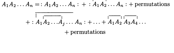 | Moyal product for Wightman propagator | |
| perturbative expansion of 3) via 1) | Feynman diagrams 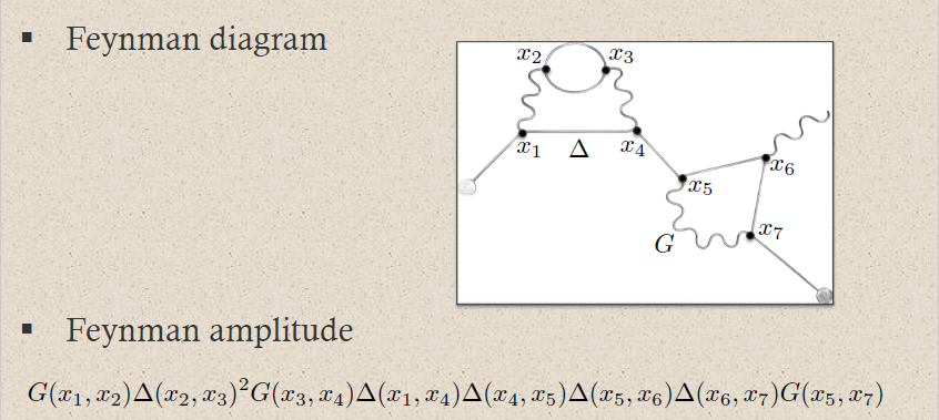 | Moyal product for Feynman propagator |
While the Wick algebra with its vacuum state provides a quantization of the algebra of observables of free gauge fixed Lagrangian field theories, the possible existence of infinitesimal gauge symmetries implies that the physically relevant observables are just the gauge invariant on-shell ones, exhibited by the cochain cohomology of the BV-BRST differential . Hence to complete quantization of gauge theories, the BV-BRST differential needs to be lifted to the noncommutative algebra of quantum observables – this is called BV-BRST quantization.
To do so, we may regard the gauge fixed BRST-action functional as an interaction term, to be dealt with later via scattering theory, and hence consider quantization of just the free BV-differential . One finds that this is equal to its time-ordered version (prop. below) plus a quantum correction, called the BV-operator (def. below) or BV-Laplacian (prop. below).
Applied to observables this relation is the Schwinger-Dyson equation (prop. below), which expresses the quantum-correction to the equations of motion of the free gauge field Lagrangian field theory as seen by time-ordered products of observables (example below.)
After introducing field-interactions via scattering theory in the next chapter the quantum correction to the BV-differential by the BV-operator becomes the “quantum master equation” and the Schwinger-Dyson equation becomes the “master Ward identity”. When choosing renormalization these identities become conditions to be satisfied by renormalization choices in order for the interacting quantum BV-BRST differential, and hence for gauge invariant quantum observables, to be well defined in perturbative quantum field theory of gauge theories. This we discuss below in Renormalization.
The abstract Wick algebra of a free field theory with Green hyperbolic differential equation is directly analogous to the star product-algebra induced by a finite dimensional Kähler vector space (def. ) under the following identification of the Wightman propagator with the Kähler space-structure:
Remark
(Wightman propagator as Kähler vector space-structure)
Let be a free Lagrangian field theory whose Euler-Lagrange equation of motion is a Green hyperbolic differential equation. Then the corresponding Wightman propagator is analogous to the rank-2 tensor on a Kähler vector space as follows:
(Fredenhagen-Rejzner 15, section 3.6, Collini 16, table 2.1)
Definition
(microcausal polynomial observables)
Let be a field bundle which is a vector bundle, over some spacetime .
A polynomial observable (def. )
is called microcausal if each distributional coefficient
as above has wave front set (def. ) not containing those elements where the wave vectors are all in the closed future cone or all in the closed past cone (def. ).
We write
for the subspace of off-shell/on-shell microcausal polynomial observables inside all off-shell/on-shell polynomial observables.
The important point is that microcausal polynomial observables still contain all regular polynomial observables but also all polynomial local observables:
Example
(regular polynomial observables are microcausal)
Every regular polynomial observable (def. ) is microcausal (def. ).
Proof
By definition of regular polynomial observables, their coefficients are non-singular distributions and because the wave front set of non-singular distributions is empty (example )
Example
(polynomial local observables are microcausal)
Every polynomial local observable (def. ) is a microcausal polynomial observable (def. ).
Proof
For notational convenience, consider the case of the scalar field with ; the general case is directly analogous. Then the local observable coming from (a phi^n interaction-term), has, regarded as a polynomial observable, the delta distribution as coefficient in degree 2:
Now for and a chart around this point, the Fourier transform of distributions of restricted to this chart is proportional to the Fourier transform of evaluated at the sum of the two covectors:
Since is a plain bump function, its Fourier transform is quickly decaying (according to prop. ) along , as long as . Only on the cone the Fourier transform is constant, and hence in particular not decaying.
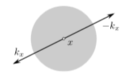
This means that the wave front set consists of the elements of the form with . Since and are both in the closed future cone or both in the closed past cone precisely if , this situation is excluded in the wave front set and hence the distribution is microcausal.
(graphics grabbed from Khavkine-Moretti 14, p. 45)
Proposition
(Hadamard-Moyal star product on microcausal observables – abstract Wick algebra)
Let a free Lagrangian field theory with Green hyperbolic equations of motion . Write for the causal propagator and let
be a corresponding Wightman propagator (Hadamard 2-point function).
Then the star product induced by
on off-shell microcausal observables (def. ) is well defined in that the wave front sets involved in the products of distributions that appear in expanding out the exponential satisfy Hörmander's criterion.
Hence by the general properties of star products (prop. ) this yields a unital associative algebra structure on the space of formal power series in of off-shell microcausal observables
This is the off-shell Wick algebra corresponding to the choice of Wightman propagator .
Moreover the image of is an ideal with respect to this algebra structure, so that it descends to the on-shell microcausal observables to yield the on-shell Wick algebra
Finally, under complex conjugation these are star algebras in that
(e.g. Collini 16, p. 25-26)
Proof
By prop. the wave front set of has all cotangents on the first variables in the closed future cone (at the given base point, which itself is on the light cone)
and hence all those on the second variables in the closed past cone.
The first variables are integrated against those of and the second against . By definition of microcausal observables (def. ), the wave front sets of and are disjoint from the subsets where all components are in the closed future cone or all components are in the closed past cone. Therefore the relevant sum of of the wave front covectors never vanishes and hence Hörmander's criterion (prop. ) for partial products of distributions of several variables (prop. ).
It remains to see that the star product is itself again a microcausal observable. It is clear that it is again a polynomial observable and that it respects the ideal generated by the equations of motion. That it still satisfies the condition on the wave front set follows directly from the fact that the wave front set of a product of distributions is inside the fiberwise sum of elements of the factor wave front sets (prop. , prop. ).
Finally the star algebra-structure via complex conjugation follows via remark as in prop. .
Remark
(Wick algebra is formal deformation quantization of Poisson-Peierls algebra of observables)
Let a free Lagrangian field theory with Green hyperbolic equations of motion with causal propagator and let be a corresponding Wightman propagator (Hadamard 2-point function).
Then the Wick algebra from prop. is a formal deformation quantization of the Poisson algebra on the covariant phase space given by the on-shell polynomial observables equipped with the Poisson-Peierls bracket in that for all we have
and
(Dito 90, Dütsch-Fredenhagen 00, Dütsch-Fredenhagen 01, Hirshfeld-Henselder 02)
Proof
By prop. this is immediate from the general properties of the star product (example ).
Explicitly, consider, without restriction of generality, and be two linear observables. Then
Now since is skew-symmetric while is symmetric (prop. ) it follows that
The right hand side is the integral kernel-expression for the Poisson-Peierls bracket, as shown in the second line.
Definition
(time-ordered product on regular polynomial observables)
Let be a free Lagrangian field theory over a Lorentzian spacetime and with Green-hyperbolic Euler-Lagrange differential equations; write for the induced causal propagator. Let moreover be a compatible Wightman propagator and write for the induced Feynman propagator.
Then the time-ordered product on the space of off-shell regular polynomial observable is the star product induced by the Feynman propagator (via prop. ):
hence
(Notice that this does not descend to the on-shell observables, since the Feynman propagator is not a solution to the homogeneous equations of motion.)
Proposition
(time-ordered product is indeed causally ordered Wick algebra product)
Let be a free Lagrangian field theory over a Lorentzian spacetime and with Green-hyperbolic Euler-Lagrange differential equations; write for the induced causal propagator. Let moreover be a compatible Wightman propagator and write for the induced Feynman propagator.
Then the time-ordered product on regular polynomial observables (def. ) is indeed a time-ordering of the Wick algebra product in that for all pairs of regular polynomial observables
with disjoint spacetime support we have
Here is the causal order relation (“ does not intersect the past cone of ”). Beware that for general pairs of subsets neither nor .
Proof
Recall the following facts:
-
the advanced and retarded propagators by definition are supported in the future cone/past cone, respectively
-
they turn into each other under exchange of their arguments (cor. ):
-
the real part of the Feynman propagator, which by definition is the real part of the Wightman propagator is symmetric (by definition or else by prop. ):
Using this we compute as follows:
Proposition
(time-ordered product on regular polynomial observables isomorphic to pointwise product)
The time-ordered product on regular polynomial observables (def. ) is isomorphic to the pointwise product of observables (def. ) via the linear isomorphism
given by
in that
hence
(Brunetti-Dütsch-Fredenhagen 09, (12)-(13), Fredenhagen-Rejzner 11b, (14))
Proof
Since the Feynman propagator is symmetric (prop. ), the statement is a special case of prop. .
Example
(time-ordered exponential of regular polynomial observables)
Let be a regular polynomial observable (def. ) of degree zero, and write
for the exponential of with respect to the pointwise product (89).
Then the exponential of with respect to the time-ordered product (def. ) is equal to the conjugation of the exponential with respect to the pointwise product by the time-ordering isomorphism from prop. :
Remark
(renormalization of time-ordered product)
The time-ordered product on regular polynomial observables from prop. extends to a product on polynomial local observables (def. ), then taking values in microcausal observables (def. ):
This extension is not unique. A choice of such an extension, satisfying some evident compatibility conditions, is a choice of renormalization scheme for the given perturbative quantum field theory. Every such choice corresponds to a choice of perturbative S-matrix for the theory, namely an extension of the time-ordered exponential (example ) from regular to local observables.
This construction of perturbative quantum field theory is called causal perturbation theory. We discuss this below in the chapters Interacting quantum fields and Renormalization.
operator product notation
Definition
(notation for operator product and normal-ordered product)
It is traditional to use the following alternative notation for the product structures on microcausal polynomial observables:
-
The Wick algebra-product, hence the star product for the Wightman propagator (def. ), is rewritten as plain juxtaposition:
-
The pointwise product of observables (def. ) is equivalently written as plain juxtaposition enclosed by colons:
-
The time-ordered product, hence the star product for the Feynman propagator (def. ) is equivalently written as plain juxtaposition prefixed by a “”
Under representation of the Wick algebra on a Fock Hilbert space by linear operators the first product becomes the operator product, while the second becomes the operator poduct applied after suitable re-ordering, called “normal odering” of the factors.
Disregarding the Fock space-representation, which is faithful, we may still refer to these “abstract” products as the “operator product” and the “normal-ordered product”, respectively.
Example
Consider phi^n theory from example . The adiabatically switched action functional (example ) which is the transgression of the phi^n interaction is the following local (hence, by example , microcausal) observable:
Here in the first line we have the integral over a pointwise product (def. ) of field observables (example ), which in the second line we write equivalently as a normal ordered product by def. .
Example
Consider the Lagrangian field theory defining quantum electrodynamics from example . The adiabatically switched action functional (example ) which is the transgression of the electron-photon interaction is the local (hence, by example , microcausal) observable
Here in the first line we have the integral over a pointwise product (def. ) of field observables (example ), which in the second line we write equivalently as a normal ordered product by def. .
(e.g. Scharf 95, (3.3.1))
Proposition
(canonical vacuum states on abstract Wick algebra)
Let be a free Lagrangian field theory with Green-hyperbolic Euler-Lagrange equations of motion; and let be a compatible Wightman propagator.
For
any on-shell field history (i.e. solving the equations of motion), consider the function from the Wick algebra to formal power series in with coefficients in the complex numbers which evaluates any microcausal polynomial observable on
Specifically for (which is a solution of the equations of motion by the assumption that defines a free field theory) this is the function
which sends each microcausal polynomial observable to its value on the zero field history, hence to the constant contribution in its polynomial expansion.
The function is
-
linear over ;
-
real, in that for all
-
positive, in that for every there exist a such that
-
normalized, in that
where denotes componet-wise complex conjugation.
This means that is a state on the Wick star-algebra (prop. ). One says that
- is a Hadamard vacuum state;
and generally
- is called a coherent state.
(Dütsch 18, def. 2.12, remark 2.20, def. 5.28, exercise 5.30 and equations (5.178))
Proof
The properties of linearity, reality and normalization are obvious, what requires proof is positivity. This is proven by exhibiting a representation of the Wick algebra on a Fock Hilbert space (this algebra homomorphism is Wick's lemma), with formal powers in suitably taken care of, and showing that under this representation the function is represented, degreewise in , by the inner product of the Hilbert space.
Example
(operator product of two linear observables)
Let
for be two linear microcausal observables represented by distributions which in generalized function-notation are given by
Then their Hadamard-Moyal star product (prop. ) is the sum of their pointwise product with their value
in the Wightman propagator, which is the value of the Hadamard vacuum state from prop. :
In the operator product/normal-ordered product-notation of def. this reads
Example
Let a free Lagrangian field theory with Green hyperbolic equations of motion and with Wightman propagator .
Then for
two linear microcausal observables, the Hadamard-Moyal star product (def. ) of their exponentials exhibits the Weyl relations:
where on the right we have the exponential of the value of the Hadamard vacuum state (prop. ) as in example .
(e.g. Dütsch 18, exercise 2.3)
Example
(Wightman propagator is 2-point function in the Hadamard vacuum state)
Let be a free Lagrangian field theory with Green-hyperbolic Euler-Lagrange equations of motion; and let be a compatible Wightman propagator.
With respect to the induced Hadamard vacuum state from prop. , the Wightman propagator itself is the 2-point function, namely the distributional vacuum expectation value of the operator product of two field observables:
Equivalently in the operator product-notation of def. this reads:
Similarly:
Example
(Feynman propagator is time-ordered 2-point function in the Hadamard vacuum state)
Let be a free Lagrangian field theory with Green-hyperbolic Euler-Lagrange equations of motion; and let be a compatible Wightman propagator with induced Feynman propagator .
With respect to the induced Hadamard vacuum state from prop. , the Feynman propagator itself is the time-ordered 2-point function, namely the distributional vacuum expectation value of the time-ordered product (def. ) of two field observables:
Equivalently in the operator product-notation of def. this reads:
propagators (i.e. integral kernels of Green functions)
for the wave operator and Klein-Gordon operator
on a globally hyperbolic spacetime such as Minkowski spacetime:
So far we have discussed the plain (graded-commutative) algebra of quantum observables of a gauged fixed free Lagrangian field theory, deforming the commutative pointwise product of observables. But after gauge fixing, the algebra of observables is not just a (graded-commutative) algebra, but carries also a differential making it a differential graded-commutative superalgebra: the global BV-differential (def. ). The gauge invariant on-shell observables are (only) the cochain cohomology of this differential. Here we discuss what becomes of this differential as we pass to the non-commutative Wick-algebra of quantum observables.
Proposition
(global BV-differential on Wick algebra)
Let be a free Lagrangian field theory (def. ) with gauge fixed BV-BRST Lagrangian density (def. ) on a graded BV-BRST field bundle (remark ). Let be a compatible Wightman propagator (def. ).
Then the global BV-differential (def. ) restricts from polynomial observables to a linear map on microcausal polynomial observables (def. )
and as such is a derivation not only for the pointwise product, but also for the product in the Wick algebra (the star product induced by the Wightman propagator):
We call regarded as a nilpotent derivation on the Wick algebra this way the free quantum BV-differential.
(Fredenhagen-Rejzner 11b, below (37), Rejzner 11, below (5.28))
Proof
By example the action of on polyomial observables is to replace antifield field observables by
where is a differential operator. By partial integration this translates to acting by the formally adjoint differential operator (def. ) via distributional derivative on the distributional coefficients of the given polynomial observable.
Now by prop. the application of retains or shrinks the wave front set of the distributional coefficient, hence it preserves the microcausality condition (def. ). This makes restrict to microcausal polynomial observables.
To see that thus restricted is a derivation of the Wick algebra product, it is sufficient to see that its commutators with the Wightman propagator vanish in each argument:
and
Because with this we have:
Here in the first step we used that is a derivation with respect to the pointwise product, by construction (def. ) and then we used the vanishing of the above commutators.
To see that these commutators indeed vanish, use that by example we have
and similarly for the other order of the tensor products. Here the term over the brace vanishes by the fact that the Wightman propagator is a solution to the homogeneous equations of motion by prop. .
To analyze the behaviour of the free quantum BV-differential in general and specifically after passing to interacting field theory (below in chapter Interacting quantum fields) it is useful to re-express it in terms of the incarnation of the global antibracket with respect not to the pointwise product of observables, but the time-ordered product:
Definition
Let be a free Lagrangian field theory (def. ) with gauge fixed BV-BRST Lagrangian density (def. ) on a graded BV-BRST field bundle (remark ).
Then the time-ordered global antibracket on regular polynomial observables
is the conjugation of the global antibracket (def. ) by the time-ordering operator (from prop. ):
hence
(Fredenhagen-Rejzner 11, (27), Rejzner 11, (5.14))
Proposition
(time-ordered antibracket with gauge fixed action functional)
Let be a free Lagrangian field theory (def. ) with gauge fixed BV-BRST Lagrangian density (def. ) on a graded BV-BRST field bundle (remark ).
Then the time-ordered antibracket (def. ) with the gauge fixed BV-action functional (def. ) equals the conjugation of the global BV-differential with the isomorphism from the pointwise to the time-ordered product of observables (from prop. )
hence
Proof
By the assumption that is a free field theory its Euler-Lagrange equations are linear in the fields, and hence is quadratic in the fields. This means that
where the second term on the right is independent of the fields, and hence that
This implies the claim:
Definition
(BV-operator for gauge fixed free Lagrangian field theory)
Let be a free Lagrangian field theory (def. ) with gauge fixed BV-BRST Lagrangian density (def. ) on a graded BV-BRST field bundle (remark ) and with corresponding gauge-fixed global BV-BRST differential on graded regular polynomial observables
Then the corresponding BV-operator
on regular polynomial observables is, up to a factor of , the difference between the free component of the gauge fixed global BV differential and its time-ordered version (def. )
hence
Proposition
(BV-operator in components)
If the field bundles of all fields, ghost fields and auxiliary fields are trivial vector bundles, with field/ghost-field/auxiliary-field coordinates collectively denoted then the BV-operator from prop. is given explicitly by
Since this formula exhibits a graded Laplace operator, the BV-operator is also called the BV-Laplace operator or BV-Laplacian, for short.
(Fredenhagen-Rejzner 11, (29), Rejzner 11, (5.20))
Proof
and by example the second term on the right is
With this we compute as follows:
Here we used
-
under the first brace that by assumption of a free field theory, is linear in the fields, so that the first commutator with the Feynman propagator is independent of the fields, and hence all the higher commutators vanish;
-
under the second brace that the Feynman propagator is times the Green function for the Green hyperbolic Euler-Lagrange equations of motion (cor. ).
Proposition
(global antibracket exhibits failure of BV-operator to be a derivation)
Let be a free Lagrangian field theory (def. ) with gauge fixed BV-BRST Lagrangian density (def. ) on a graded BV-BRST field bundle
The BV-operator (def. ) and the global antibracket (def. ) satisfy for all polynomial observables (def. ) the relation
for the pointwise product of observables (def. ).
Moreover, it commutes on regular polynomial observables with the time-ordering operator (prop. )
and hence satisfies the analogue of relation (223) also for the time-ordered antibracket (def. ) and the time-ordered product on regular polynomial observables
(e.g. Henneaux-Teitelboim 92, (15.105d))
Proof
With prop. the first statement is a graded version of the analogous relation for an ordinary Laplace operator acting on smooth functions on Cartesian space, which on smooth functions satisfies
by the product law for differentiation, where now is the gradient and the inner product. Here one just needs to carefully record the relative signs that appear.
That the BV-operator commutes with the time-ordering operator is clear from the fact that both of these are given by partial functional derivatives with constant coefficients. This immediately implies the last statement from the first.
Example
(BV-operator on time-ordered exponentials)
Let be a free Lagrangian field theory (def. ) with gauge fixed BV-BRST Lagrangian density (def. ) on a graded BV-BRST field bundle .
Let moreover be a regular polynomial observable (def. ) of degree zero. Then the application of the BV-operator (def. ) to the time-ordered exponential (example ) is the time-ordered product of the time-ordered exponential with the sum of and the global antibracket of with itself:
Proof
By prop. acts as a derivation on the time-ordered product up to a correction given by the antibracket of the two factors. This yields the result by the usual combinatorics of exponentials.
A special case of the general occurrence of the BV-operator is the following important property of on-shell time-ordered products:
Proposition
Let be a free Lagrangian field theory (def. ) with gauge fixed BV-BRST Lagrangian density (def. ) on a graded BV-BRST field bundle (remark ).
Let
be an off-shell regular polynomial observable which is linear in the antifield field observables . Then
This is called the Schwinger-Dyson equation.
The following proof is due to (Rejzner 16, remark 7.7) following the informal traditional argument (Henneaux-Teitelboim 92, (15.108b)).
Proof
Applying the inverse time-ordering map (prop. ) to equation (221) applied to yields
where we have identified the terms under the braces by 1) the component expression for the BV-differential from prop. , 2) prop. and 3) prop. .
The last term is manifestly in the image of the BV-differential and hence vanishes when passing to on-shell observables along the isomorphism (198)
The same argument with the replacement throughout yields the other version of the equation (with time-ordering instead of reverse time ordering and the sign of the -term reversed).
Remark
(“Schwinger-Dyson operator”)
The proof of the Schwinger-Dyson equation in prop. shows that, up to time-ordering, the Schwinger-Dyson equation is the on-shell vanishing of the “quantized” BV-differential (221)
where the BV-operator is the quantum correction of order . Therefore this is also called the Schwinger-Dyson operator (Henneaux-Teitelboim 92, (15.111)).
Example
(distributional Schwinger-Dyson equation)
Often the Schwinger-Dyson equation (prop. ) is displayed before spacetime-smearing of field observables in terms of operator products of operator-valued distributions, taking the observable in (224) to be
This choice makes (225) become the distributional Schwinger-Dyson equation
(e.q. Dermisek 09).
In particular this means that if for all then
Since by the principle of extremal action (prop. ) the equation
is the Euler-Lagrange equation of motion (for the classical field theory) “at ”, this may be interpreted as saying that the classical equations of motion for fields at still hold for time-ordered quantum expectation values, as long as all other observables are evaluated away from ; while if observables do coincide at then there is a correction measured by the BV-operator.
This concludes our discussion of the algebra of quantum observables for free field theories. In the next chapter we discuss the perturbative QFT of interacting field theories as deformations of such free quantum field theories.
Interacting quantum fields
In this chapter we discuss the following topics:
In the previous chapter we have found the quantization of free Lagrangian field theories by first choosing a gauge fixed BV-BRST-resolution of the algebra of gauge invariant on-shell observabes, then applying algebraic deformation quantization induced by the resulting Peierls-Poisson bracket on the graded covariant phase space to pass to a non-commutative algebra of quantum observables, such that, finally, the BV-BRST differential is respected.
Of course most quantum field theories of interest are non-free; they are interacting field theories whose equations of motion is a non-linear differential equation. The archetypical example is the coupling of the Dirac field to the electromagnetic field via the electron-photon interaction, corresponding to the interacting field theory called quantum electrodynamics (discussed below).
In principle, the perturbative quantization of such non-free interacting field theories proceeds the same way: One picks a BV-BRST-gauge fixing, computes the Peierls-Poisson bracket on the resulting covariant phase space (Khavkine 14) and then finds a formal deformation quantization of this Poisson structure to obtain the quantized non-commutative algebra of quantum observables, as formal power series in Planck's constant .
It turns out (Collini 16, Hawkins-Rejzner 16, prop. below) that the resulting interacting formal deformation quantization may equivalently be expressed in terms of scattering amplitudes (example below): These are the probability amplitudes for plane waves of free fields to come in from the far past, then interact in a compact region of spacetime via the given interaction (adiabatically switched-off outside that region) and to emerge again as free fields into the far future.
The collection of all these scattering amplitudes, as the types and wave vectors of the incoming and outgoing free fields varies, is called the perturbative scattering matrix of the interacting field theory, or just S-matrix for short. It may equivalently be expressed as the exponential of time-ordered products of the adiabatically switched interaction action functional with itself (def. below). The combinatorics of the terms in this exponential is captured by Feynman diagrams (prop. below), which, with some care (remark below), may be thought of as finite multigraphs (def. below) whose edges are worldlines of virtual particles and whose vertices are the interactions that these particles undergo (def. below).
The axiomatic definition of S-matrices for relativistic Lagrangian field theories and their rigorous construction via ("re"-)normalization of time-ordered products (def. below) is called causal perturbation theory, due to (Epstein-Glaser 73). This makes precise and well-defined the would-be path integral quantization of interacting field theories (remark below) and removes the errors (remark below) and ensuing puzzlements (expressed in Feynman 85) that plagued the original informal conception of perturbative quantum field theory due to Schwinger-Tomonaga-Feynman-Dyson (remark below).
The equivalent re-formulation of the formal deformation quantization of interacting field theories in terms of scattering amplitudes (prop. below) has the advantage that it gives a direct handle on those observables that are measured in scattering experiments, such as the LHC-experiment. The bulk of mankind’s knowledge about realistic perturbative quantum field theory – such as notably the standard model of particle physics – is reflected in such scattering amplitudes given via their Feynman perturbation series in formal powers of Planck's constant and the coupling constant.
Moreover, the mathematical passage from scattering amplitudes to the actual interacting field algebra of quantum observables (def. below) corresponding to the formal deformation quantization is well understood, given via “Bogoliubov's formula” by the quantum Møller operators (def. below).
Via Bogoliubov's formula every perturbative S-matrix scheme (def. ) induces for every choice of adiabatically switched interaction action functional a notion of perturbative interacting field observables (def. ). These generate an algebra (def. below). By Bogoliubov's formula, in general this algebra depends on the choice of adiabatic switching; which however is not meant to be part of the physics, but just a mathematical device for grasping global field structures locally.
But this spurious dependence goes away (prop. below) when restricting attention to observables whose spacetime support is inside a compact causally closed subsets of spacetime (def. below). This is a sensible condition for an observable in physics, where any realistic experiment nessecarily probes only a compact subset of spacetime, see also remark .
The resulting system (a “co-presheaf”) of well-defined perturbative interacting field algebras of observables (def. below)
is in fact causally local (prop. below). This fact was presupposed without proof already in Il’in-Slavnov 78; because this is one of two key properties that the Haag-Kastler axioms (Haag-Kastler 64) demand of an intrinsically defined quantum field theory (i.e. defined without necessarily making recourse to the geometric backdrop of Lagrangian field theory). The only other key property demanded by the Haag-Kastler axioms is that the algebras of observables be C*-algebras; this however must be regarded as the axiom encoding non-perturbative quantum field theory and hence is necessarily violated in the present context of perturbative QFT. Since quantum field theory following the full Haag-Kastler axioms is commonly known as AQFT, this perturbative version, with causally local nets of observables but without the C*-algebra-condition on them, has come to be called perturbative AQFT (Dütsch-Fredenhagen 01, Fredenhagen-Rejzner 12).
In this terminology the content of prop. below is that while the input of causal perturbation theory is a gauge fixed Lagrangian field theory, the output is a perturbative algebraic quantum field theory:
The independence of the causally local net of localized interacting field algebras of observables from the choice of adiabatic switching implies a well-defined spacetime-global algebra of observables by forming the inductive limit
This is also called the algebraic adiabatic limit, defining the algebras of observables of perturbative QFT “in the infrared”. The only remaining step in the construction of a perturbative QFT that remains is then to find an interacting vacuum state
on the global interacting field algebra . This is related to the actual adiabatic limit, and it is by and large an open problem, see remark below.
In conclusion so far, the algebraic adiabatic limit yields, starting with a BV-BRST gauge fixed free field vacuum, the perturbative construction of interacting field algebras of observables (def. ) and their organization in increasing powers of and (loop order, prop. ) via the Feynman perturbation series (example , example ).
But this interacting field algebra of observables still involves all the auxiliary fields of the BV-BRST gauge fixed free field vacuum (as in example for QED), while the actual physical gauge invariant on-shell observables should be (just) the cochain cohomology of the BV-BRST differential on this enlarged space of observables. Hence for the construction of perturbative QFT to conclude, it remains to pass the BV-BRST differential of the free field Wick algebra of observables to a differential on the interacting field algebra, such that its cochain cohomology is well defined.
Since the time-ordered products away from coinciding interaction points are uniquely fixed (prop. below), one finds that also this interacting quantum BV-differential is uniquely fixed, on regular polynomial observables, by conjugation with the quantum Møller operators (def. ). The formula that characterizes it there is called the quantum master equation or equivalently the quantum master Ward identity (prop. below).
In its incarnation as the master Ward identity, this expresses the difference between the shell of the free classical field theory and that of the interacting quantum field theory, thus generalizing the Schwinger-Dyson equation to interacting field theory (example below). Applied to Noether's theorem it expresses the possible failure of conserved currents associated with infinitesimal symmetries of the Lagrangian to still be conserved in the interacting perturbative QFT (example below).
As one extends the time-ordered products to coinciding interaction points in ("re"-)normalization of the perturbative QFT (def. below), the quantum master equation/master Ward identity becomes a renormalization condition (prop. below). If this condition fails one says that the interacting perturbative QFT has a quantum anomaly, specifically a gauge anomaly if the Ward identity of an infinitesimal gauge symmetry is violated.
These issues of "(re)-"normalization we discuss in detail in the next chapter.
Free field vacua
In considering perturbative QFT, we are considering perturbation theory in formal deformation parameters around a fixed free Lagrangian quantum field theory in a chosen Hadamard vacuum state.
For convenient referencing we collect all the structure and notation that goes into this in the following definitions:
Definition
(free relativistic Lagrangian quantum field vacuum)
Let
-
be a spacetime (e.g. Minkowski spacetime);
-
a free Lagrangian field theory (def. ), with field bundle ;
-
a gauge parameter bundle for (def. ), with induced BRST-reduced Lagrangian field theory (example );
-
a gauge fixing (def. ) with graded BV-BRST field bundle (remark );
-
a Wightman propagator compatible with the causal propagator which corresponds to the Green hyperbolic Euler-Lagrange equations of motion induced by the gauge-fixed Lagrangian density .
Given this, we write
for the corresponding Wick algebra-structure on formal power series in (Planck's constant) of microcausal polynomial observables (def. ). This is a star algebra with respect to (coefficient-wise) complex conjugation (prop. ).
Write
for the induced Hadamard vacuum state (prop. ), hence the state whose distributional 2-point function is the chosen Wightman propagator:
Given any microcausal polynomial observable then its value in this state is called its free vacuum expectation value
Write
for the inclusion of local observables (def. ) into microcausal polynomial observables (example ), thought of as forming normal-ordered products in the Wick algebra (by def. ).
We denote the Wick algebra-product (the star product induced by the Wightman propagator according to prop. ) by juxtaposition (def. )
If an element has an inverse with respect to this product, we denote that by :
Finally, for we write for its spacetime support (def. ). For two subsets of spacetime we write
for the causal order-relation (def. ) and
for spacelike separation.
Being concerned with perturbation theory means mathematically that we consider formal power series in deformation parameters (“Planck's constant”) and (“coupling constant”), also in (“source field”), see also remark . The following collects our notational conventions for these matters:
Definition
(formal power series of observables for perturbative QFT)
Let be a relativistic free vacuum according to def. .
Write
for the space of formal power series in three formal variables
-
(“Planck's constant”),
-
(“source field”)
with coefficients in the topological vector spaces of the off-shell polynomial local observables of the free field theory (def. ); similarly for the off-shell microcausal polynomial observables (def. ):
Similary
denotes the subspace for which no powers of appear, etc.
Accordingly
denotes the vector space of bump functions on spacetime tensored with the vector space spanned by a single copy of . The elements
may be regarded as spacetime-dependent “coupling constants” with compact support, called adiabatically switched couplings.
Similarly then
is the subspace of those formal power series that are at least linear in or (hence those that vanish if one sets ). Hence every element of this space may be written in the form
where the notation is to suggest that we will think of the coefficient of as an (adiabatically switched) interaction action functional and of the coefficient of as an external source field (reflected by internal and external vertices, respectively, in Feynman diagrams, see def. below).
In particular for
a formal power series in and of local Lagrangian densities (def. ), thought of as a local interaction Lagrangians, and if
is an adiabatically switched coupling as before, then the transgression (def. ) of the product
is such an adiabatically switched interaction
We also consider the space of off-shell microcausal polynomial observables of the free field theory with formal parameters adjoined
which, in its -dependent, is the space of Laurent series in , hence the space exhibiting also negative formal powers of .
Perturbative S-Matrices
We introduce now the axioms for perturbative scattering matrices relative to a fixed relativistic free Lagrangian quantum field vacuum (def. below) according to causal perturbation theory (def. below). Since the first of these axioms requires the S-matrix to be a formal sum of multi-linear continuous functionals, it is convenient to impose axioms on these directly: this is the axiomatics for time-ordered products in def. below. That these latter axioms already imply the former is the statement of prop. , prop. below . Its proof requires a close look at the “reverse-time ordered products” for the inverse S-matrix (def. below) and their induced reverse-causal factorization (prop. below).
Definition
(S-matrix axioms – causal perturbation theory)
Let be a relativistic free vacuum according to def. .
Then a perturbative S-matrix scheme for perturbative QFT around this free vacuum is a function
from local observables to microcausal polynomial observables of the free vacuum theory, with formal parameters adjoined as indicated (def. ), such that the following two conditions “perturbation” and “causal additivity (jointly: ”causal perturbation theory“) hold:
-
There exist multi-linear continuous functionals (over ) of the form
(228)for all , such that:
-
The nullary map is constant on the unit of the Wick algebra
-
The unary map is the inclusion of local observables as normal-ordered products (227)
-
The perturbative S-matrix is the exponential series of these maps in that for all
(229)
-
-
For all perturbative local observables we have
(230)
(The inverse of with respect to the Wick algebra-structure is implied to exist by the axiom “perturbation”, see remark below.)
Def. is due to (Epstein-Glaser 73 (1)), following (Stückelberg 49-53, Bogoliubov-Shirkov 59). That the domain of an S-matrix scheme is indeed the space of local observables was made explicit (in terms of axioms for the time-ordered products, see def. below), in (Brunetti-Fredenhagen 99, section 3, Dütsch-Fredenhagen 04, appendix E, Hollands-Wald 04,around (20)). Review includes (Rejzner 16, around def. 6.7, Dütsch 18, section 3.3).
Remark
(invertibility of the S-matrix)
The mutliplicative inverse of the perturbative S-matrix in def. with respect to the Wick algebra-product indeed exists, so that the list of axioms is indeed well defined: By the axiom “perturbation” this follows with the usual formula for the multiplicative inverse of formal power series that are non-vanishing in degree 0:
If we write
then
where the sum does exist in , because (by the axiom “perturbation”) has vanishing coefficient in zeroth order in the formal parameters and , so that only a finite sub-sum of the formal infinite sum contributes in each order in and .
This expression for the inverse of S-matrix may usefully be re-organized in terms of “rever-time ordered products” (def. below), see prop. below.
Notice that is instead the inverse with respect to the time-ordered products (228) in that
(Since the time-ordered product is, by definition, symmetric in its arguments, the usual formula for the multiplicative inverse of an exponential series applies).
Remark
(adjoining further deformation parameters)
The definition of S-matrix schemes in def. has immediate variants where arbitrary countable sets and of formal deformation parameters are considered, instead of just a single coupling constant and a single source field . The more such constants are considered, the “more perturbative” the theory becomes and the stronger the implications.
Given a perturbative S-matrix scheme (def. ) it immediately induces a corresponding concept of observables:
Definition
(generating function scheme for interacting field observables)
Let be a relativistic free vacuum according to def. , let be a corresponding S-matrix scheme according to def. .
The corresponding generating function scheme (for interacting field observables, def. below) is the functional
given by
Proposition
(causal additivity in terms of generating functions)
In terms of the generating functions (def. ) the axiom “causal additivity” on the S-matrix scheme (def. ) is equivalent to:
-
(causal additivity in terms of )
For all local observables we have
(233)
(Whence “additivity”.)
Proof
This follows by elementary manipulations:
Multiplying both sides of (230) by yields
This is the first line of (233).
Multiplying both sides of (230) by yields
This is the second line of (233).
Definition
(interacting field observables – Bogoliubov's formula)
Let be a relativistic free vacuum according to def. , let be a corresponding S-matrix scheme according to def. , and let be a local observable regarded as an adiabatically switched interaction-functional.
Then for a local observable of the free field theory, we say that the corresponding local interacting field observable
is the coefficient of in the generating function (232):
This expression is called Bogoliubov's formula, due to (Bogoliubov-Shirkov 59).
One thinks of as the deformation of the local observable as the interaction is turned on; and speaks of an element of the interacting field algebra of observables. Their value (“expectation value”) in the given free Hadamard vacuum state (def. ) is a formal power series in Planck's constant and in the coupling constant , with coefficients in the complex numbers
which express the probability amplitudes that reflect the predictions of the perturbative QFT, which may be compared to experiment.
(Epstein-Glaser 73, around (74)); review includes (Dütsch-Fredenhagen 00, around (17), Dütsch 18, around (3.212)).
Remark
(interacting field observables are formal deformation quantization)
The interacting field observables in def. are indeed formal power series in the formal parameter (Planck's constant), as opposed to being more general Laurent series, hence they involve no negative powers of (Dütsch-Fredenhagen 00, prop. 2 (ii), Hawkins-Rejzner 16, cor. 5.2). This is not immediate, since by def. the S-matrix that they are defined from does involve negative powers of .
It follows in particular that the interacting field observables have a classical limit , which is not the case for the S-matrix itself (due to it involving negative powers of ). Indeed the interacting field observables constitute a formal deformation quantization of the covariant phase space of the interacting field theory (prop. below) and are thus the more fundamental concept.
As the name suggests, the S-matrices in def. serve to express scattering amplitudes (example below). But by remark the more fundamental concept is that of the interacting field observables. Their perspective reveals that consistent interpretation of scattering amplitudes requires the following condition on the relation between the vacuum state and the interaction term:
Definition
Let be a relativistic free vacuum according to def. , let be a corresponding S-matrix scheme according to def. , and let be a local observable, regarded as an adiabatically switched interaction action functional.
We say that the given Hadamard vacuum state (prop. )
is stable with respect to the interaction , if for all elements of the Wick algebra
we have
Example
(time-ordered product of interacting field observables)
Let be a relativistic free vacuum according to def. , let be a corresponding S-matrix scheme according to def. , and let be a local observable regarded as an adiabatically switched interaction-functional.
Consider two local observables
with causally ordered spacetime support
Then causal additivity according to prop. implies that the Wick algebra-product of the corresponding interacting field observables (def. ) is
Here the last line makes sense if one extends the axioms on the S-matrix in prop. from formal power series in to formal power series in (remark ). Hence in this generalization, the generating functions are not just generating functions for interacting field observables themselves, but in fact for time-ordered products of interacting field observables.
An important special case of time-ordered products of interacting field observables as in example is the following special case of scattering amplitudes, which is the example that gives the scattering matrix in def. its name:
Example
(scattering amplitudes as vacuum expectation values of interacting field observables)
Let be a relativistic free vacuum according to def. , let be a corresponding S-matrix scheme according to def. , and let be a local observable regarded as an adiabatically switched interaction-functional, such that the vacuum state is stable with respect to (def. ).
Consider local observables
whose spacetime support satisfies the following causal ordering:
for all and .
Then the vacuum expectation value of the Wick algebra-product of the corresponding interacting field observables (def. ) is
These vacuum expectation values are interpreted, in the adiabatic limit where , as scattering amplitudes (remark below).
Proof
For notational convenience, we spell out the argument for . The general case is directly analogous.
So assuming the causal order (def. )
we compute with causal additivity via prop. as follows:
With this the statement follows by the definition of vacuum stability (def. ).
Remark
(computing S-matrices via Feynman perturbation series)
For practical computation of vacuum expectation values of interacting field observables (example ) and hence in particular, via example , of scattering amplitudes, one needs some method for collecting all the contributions to the formal power series in increasing order in and .
Such a method is provided by the Feynman perturbation series (example below) and the effective action (def. ), see example below.
Conceptual remarks
The simple axioms for S-matrix schemes in causal perturbation theory (def. ) and hence for interacting field observables (def. ) have a wealth of implications and consequences. Before discussing these formally below, we here make a few informal remarks meant to put various relevant concepts into perspective:
Remark
(perturbative QFT and asymptotic expansion of probability amplitudes)
Given a perturbative S-matrix scheme (def. ), then by remark the expectation values of interacting field observables (def. ) are formal power series in the formal parameters and (which are interpreted as Planck's constant, and as the coupling constant, respectively):
This means that there is no guarantee that these series converge for any positive value of and/or . In terms of synthetic differential geometry this means that in perturbative QFT the deformation of the classical free field theory by quantum effects (measured by ) and interactions (meaured by ) is so very tiny as to actually be infinitesimal: formal power series may be read as functions on the infinitesimal neighbourhood in a space of Lagrangian field theories at the point , .
In fact, a simple argument (due to Dyson 52) suggests that in realistic field theories these series never converge for any positive value of and/or . Namely convergence for would imply a positive radius of convergence around , which would imply convergence also for and even for imaginary values of , which would however correspond to unstable interactions for which no converging field theory is to be expected. (See Helling, p. 4 for the example of phi^4 theory.)
In physical practice one tries to interpret these non-converging formal power series as asymptotic expansions of actual but hypothetical functions in , which reflect the actual but hypothetical non-perturbative quantum field theory that one imagines is being approximated by perturbative QFT methods. An asymptotic expansion of a function is a power series which may not converge, but which has for every an estimate for how far the sum of the first terms in the series may differ from the function being approximated.
For examples such as quantum electrodynamics and quantum chromodynamics, as in the standard model of particle physics, the truncation of these formal power series scattering amplitudes to the first handful of loop orders in happens to agree with experiment (such as at the LHC collider) to high precision (for QED) or at least decent precision (for QCD), at least away from infrared phenomena (see remark ).
In summary this says that perturbative QFT is an extremely coarse and restrictive approximation to what should be genuine non-perturbative quantum field theory, while at the same time it happens to match certain experimental observations to remarkable degree, albeit only if some ad-hoc truncation of the resulting power series is considered.
This is strong motivation for going beyond perturbative QFT to understand and construct genuine non-perturbative quantum field theory. Unfortunately, this is a wide-open problem, away from toy examples. Not a single interacting field theory in spacetime dimension has been non-perturbatively quantized. Already a single aspect of the non-perturbative quantization of Yang-Mills theory (as in QCD) has famously been advertized as one of the Millennium Problems of our age; and speculation about non-perturbative quantum gravity is the subject of much activity.
Now, as the name indicates, the axioms of causal perturbation theory (def. ) do not address non-perturbative aspects of non-perturbative field theory; the convergence or non-convergence of the formal power series that are axiomatized by Bogoliubov's formula (def. ) is not addressed by the theory. The point of the axioms of causal perturbation theory is to give rigorous mathematical meaning to everything else in perturbative QFT.
Remark
(Dyson series and Schrödinger equation in interaction picture)
The axiom “causal additivity” (230) on an S-matrix scheme (def. ) implies immediately this seemingly weaker condition (which turns out to be equivalent, this is prop. below):
-
For all local observables we have
(This is the special case of “causal additivity” for , using that by the axiom “perturbation” (229) we have .)
If we now think of and themselves as adiabatically switched interaction action functionals, then this becomes
This exhibits the S-matrix-scheme as a “causally ordered exponential” or “Dyson series” of the interaction, hence as a refinement to relativistic field theory of what in quantum mechanics is the “integral version of the Schrödinger equation in the interaction picture” (see this equation at S-matrix; see also Scharf 95, second half of 0.3).
The relevance of manifest causal additivity of the S-matrix, over just causal factorization (even though both conditions happen to be equivalent, see prop. below), is that it directly implies that the induced interacting field algebra of observables (def. ) forms a causally local net (prop. below).
Remark
(path integral-intuition)
In informal discussion of perturbative QFT going back to informal ideas of Schwinger-Tomonaga-Feynman-Dyson, the perturbative S-matrix is thought of in terms of a would-be path integral, symbolically written
Here the would-be integration is thought to be over the space of field histories (the space of sections of the given field bundle, remark ) for field histories which satisfy given asymptotic conditions at ; and as these boundary conditions vary the above is regarded as a would-be integral kernel that defines the required operator in the Wick algebra (e.g. Weinberg 95, around (9.3.10) and (9.4.1)). This is related to the intuitive picture of the Feynman perturbation series (example below) expressing a sum over all possible interactions of virtual particles (remark ).
Beyond toy examples, it is not known how to define the would-be measure and it is not known how to make sense of this expression as an actual integral.
The analogous path-integral intuition for Bogoliubov's formula for interacting field observables (def. ) symbolically reads
If here we were to regard the expression
as a would-be Gaussian measure on the space of field histories, normalized to a would-be probability measure, then this formula would express interacting field observables as ordinary expectation values
As before, beyond toy examples it is not known how to make sense of this as an actual integration.
But we may think of the axioms for the S-matrix in causal perturbation theory (def. ) as rigorously defining the path integral, not analytically as an actual integration, but synthetically by axiomatizing the properties of the desired outcome of the would-be integration:
The analogy with a well-defined integral and the usual properties of an exponential vividly suggest that the would-be path integral should obey causal factorization. Instead of trying to make sense of path integration so that this factorization property could then be appealed to as a consequence of general properties of integration and exponentials, the axioms of causal perturbation theory directly prescribe the desired factorization property, without insisting that it derives from an actual integration.
The great success of path integral-intuition in the development of quantum field theory, despite the dearth of actual constructions, indicates that it is not the would-be integration process as such that actually matters in field theory, but only the resulting properties that this suggests the S-matrix should have; which is what causal perturbation theory axiomatizes. Indeed, the simple axioms of causal perturbation theory rigorously imply finite (i.e. ("re"-)normalized) perturbative quantum field theory (see remark ).
Remark
Let be a relativistic free vacuum according to def. , let be a corresponding S-matrix scheme according to def. , and let
be a local observable, regarded as an adiabatically switched interaction action functional.
Then for
two microcausal polynomial observables, with causal ordering
the corresponding scattering amplitude (as in example ) is the value (called “expectation value” when referring to , or “matrix element” when referring to , or “transition amplitude” when referring to and )
for the Wick algebra-product in the given Hadamard vacuum state .
If here and are monomials in Wick algebra-products of the field observables , then this scattering amplitude comes from the integral kernel
or similarly, under Fourier transform of distributions,
These are interpreted as the (distributional) probability amplitudes for plane waves of field species with wave vector to come in from the far past, ineract with each other via , and emerge in the far future as plane waves of field species with wave vectors .
Or rather:
Remark
(adiabatic limit, infrared divergences and interacting vacuum)
Since a local observable by definition has compact spacetime support, the scattering amplitudes in remark describe scattering processes for interactions that vanish (are “adiabatically switched off”) outside a compact subset of spacetime. This constraint is crucial for causal perturbation theory to work.
There are several aspects to this:
-
(adiabatic limit) On the one hand, real physical interactions (say the electron-photon interaction) are not really supposed to vanish outside a compact region of spacetime. In order to reflect this mathematically, one may consider a sequence of adiabatic switchings (each of compact support) whose limit is the constant function (the actual coupling constant), then consider the corresponding sequence of interaction action functionals and finally consider:
-
as the true scattering amplitude the corresponding limit
of adiabatically switched scattering amplitudes (remark ) – if it exists. This is called the strong adiabatic limit.
-
as the true n-point functions the corresponding limit
of tempered distributional expectation values of products of interacting field observables (def. ) – if it exists. (Similarly for time-ordered products.) This is called the weak adiabatic limit.
Beware that the left hand sides here are symbolic: Even if the limit exists in expectation values, in general there is no actual observable whose expectation value is that limit.
The strong and weak adiabatic limits have been shown to exist if all fields are massive (Epstein-Glaser 73). The weak adiabatic limit has been shown to exists for quantum electrodynamics and for mass-less phi^4 theory (Blanchard-Seneor 75) and for larger classes of field theories in (Duch 17, p. 113, 114).
If these limits do not exist, one says that the perturbative QFT has an infrared divergence.
-
-
(algebraic adiabatic limit) On the other hand, it is equally unrealistic that an actual experiment detects phenomena outside a given compact subset of spacetime. Realistic scattering experiments (such as the LHC) do not really prepare or measure plane waves filling all of spacetime as described by the scattering amplitudes (235). Any observable that is realistically measurable must have compact spacetime support. We see below in prop. that such interacting field observables with compact spacetime support may be computed without taking the adiabatic limit: It is sufficient to use any adiabatic switching which is constant on the support of the observable.
This way one obtains for each causally closed subset of spacetime an algebra of observables whose support is in , and for each inclusion of subsets a corresponding inclusion of algebras of observables (prop. below). Of this system of observables one may form the category-theoretic inductive limit to obtain a single global algebra of observables.
This always exists. It is called the algebraic adiabatic limit (going back to Brunetti-Fredenhagen 00, section 8).
For quantum electrodynamics the algebraic adiabatic limit was worked out in (Dütsch-Fredenhagen 98, reviewed in Dütsch 18, 5,3).
-
(interacting vacuum) While, via the above algebraic adiabatic limit, causal perturbation theory yields the correct interacting field algebra of quantum observables independent of choices of adiabatic switching, a theory of quantum probability requires, on top of the algebra of observables, also a state
Just as the interacting field algebra of observables is a deformation of the free field algebra of observables (Wick algebra), there ought to be a corresponding deformation of the free Hadamard vacuum state into an “interacting vacuum state” .
Sometimes the weak adiabatic limit serves to define the interacting vacuum (see Duch 17, p. 113-114).
A stark example of these infrared issues is the phenomenon of confinement of quarks to hadron bound states (notably to protons and neutrons) at large wavelengths. This is paramount in observation and reproduced in numerical lattice gauge theory simulation, but is invisible to perturbative quantum chromodynamics in its free field vacuum state, due to infrared divergences. It is expected that this should be rectified by the proper interacting vacuum of QCD (Rafelski 90, pages 12-16), which is possibly a “theta-vacuum” exhibiting superposition of QCD instantons (Schäfer-Shuryak 98, section III.D). This remains open, closely related to the Millennium Problem of quantization of Yang-Mills theory.
In contrast to the above subtleties about the infrared divergences, any would-be UV-divergences in perturbative QFT are dealt with by causal perturbation theory:
Remark
(the traditional error leading to UV-divergences)
Naively it might seem that (say over Minkowski spacetime, for simplicity) examples of time-ordered products according to def. might simply be obtained by multiplying Wick algebra-products with step functions of the time coordinates, hence to write, in the notation as generalized functions (remark ):
and analogously for time-ordered products of more arguments (for instance Weinberg 95, p. 143, between (3.5.9) and (3.5.10)).
This however is simply a mathematical error (as amplified in Scharf 95, below (3.2.4), below (3.2.44) and in fig. 3):
Both as well as are distributions and their product of distributions is in general not defined, as Hörmander's criterion (prop. ), which is exactly what guarantees absence of UV-divergences (remark ), may be violated. The notorious ultraviolet divergences which plagued (Feynman 85) the original conception of perturbative QFT due to Schwinger-Tomonaga-Feynman-Dyson are the signature of this ill-defined product (see remark ).
On the other hand, when both distributions are restricted to the complement of the diagonal (i.e. restricted away from coinciding points ), then the step function becomes a non-singular distribution so that the above expression happens to be well defined and does solve the axioms for time-ordered products.
Hence what needs to be done to properly define the time-ordered product is to choose an extension of distributions of the above product expression back from the complement of the diagonal to the whole space of tuples of points. Any such extension will produce time-ordered products.
There are in general several different such extensions. This freedom of choice is the freedom of "re-"normalization; or equivalently, by the main theorem of perturbative renormalization theory (theorem below), this is the freedom of choosing “counterterms” (remark below) for the local interactions. This we discuss below and in more detail in the next chapter.
Remark
(absence of ultraviolet divergences and re-normalization)
The simple axioms of causal perturbation theory (def. ) do fully capture perturbative quantum field theory “in the ultraviolet”: A solution to these axioms induces, by definition, well-defined perturbative scattering amplitudes (remark ) and well-defined perturbative probability amplitudes of interacting field observables (def. ) induced by local action functionals (describing point-interactions such as the electron-photon interaction). By the main theorem of perturbative renormalization (theorem ) such solutions exist. This means that, while these are necessarily formal power series in and (remark ), all the coefficients of these formal power series (“loop order contributions”) are well defined.
This is in contrast to the original informal conception of perturbative QFT due to Schwinger-Tomonaga-Feynman-Dyson, which in a first stage produced ill-defined diverging expressions for the coefficients (due to the mathematical error discussed in remark below), which were then “re-normalized” to finite values, by further informal arguments.
Here in causal perturbation theory no divergences in the coefficients of the formal power series are considered in the first place, all coefficients are well-defined, hence “finite”. In this sense causal perturbation theory is about “finite” perturbative QFT, where instead of “re-normalization” of ill-defined expressions one just encounters “normalization” (prominently highlighted in Scharf 95, see title, introduction, and section 4.3), namely compatible choices of these finite values. The actual “re-normalization” in the sense of “change of normalization” is expressed by the Stückelberg-Petermann renormalization group.
This refers to those divergences that are known as UV-divergences, namely short-distance effects, which are mathematically reflected in the fact that the perturbative S-matrix scheme (def. ) is defined on local observables, which, by their very locality, encode point-interactions. See also remark on infrared divergences.
Remark
(virtual particles, worldline formalism and perturbative string theory)
It is suggestive to think of the edges in the Feynman diagrams (def. ) as worldlines of “virtual particles” and of the vertices as the points where they collide and transmute. (Care must be exercised not to confuse this with concepts of real particles.) With this interpretation prop. may be read as saying that the scattering amplitude for given external source fields (remark ) is the superposition of the Feynman amplitudes of all possible ways that these may interact; which is closely related to the intuition for the path integral (remark ).
This intuition is made precise by the worldline formalism of perturbative quantum field theory (Strassler 92). This is the perspective on perturbative QFT which directly relates perturbative QFT to perturbative string theory (Schmidt-Schubert 94). In fact the worldline formalism for perturbative QFT was originally found by taking thre point-particle limit of string scattering amplitudes (Bern-Kosower 91, Bern-Kosower 92).
Remark
Beware the terminology in def. : A single S-matrix is one single observable
for a fixed (adiabatically switched local) interaction , reflecting the scattering amplitudes (remark ) with respect to that particular interaction. Hence the function
axiomatized in def. is really a whole scheme for constructing compatible S-matrices for all possible (adiabatically switched, local) interactions at once.
Since the usual proof of the construction of such schemes of S-matrices involves ("re"-)normalization, the function axiomatized by def. may also be referred to as a ("re"-)normalization scheme.
This perspective on as a renormalization scheme is amplified by the main theorem of perturbative renormalization (theorem ) wich states that the space of choices for is a torsor over the Stückelberg-Petermann renormalization group.
Remark
The axioms for the S-matrix in def. (and similarly that for the time-ordered products below in def. ) are sufficient to imply a causally local net of perturbative interacting field algebras of quantum observables (prop. below), and thus its algebraic adiabatic limit (remark ).
It does not guarantee, however, that the BV-BRST differential passes to those algebras of quantum observables, hence it does not guarantee that the infinitesimal symmetries of the Lagrangian are respected by the quantization process (there may be “quantum anomalies”). The extra condition that does ensure this is the quantum master Ward identity or quantum master equation. This we discuss elsewhere.
Apart from gauge symmetries one also wants to require that rigid symmetries are preserved by the S-matrix, notably Poincare group-symmetry for scattering on Minkowski spacetime.
Interacting field observables
We now discuss how the perturbative interacting field observables which are induced from an S-matrix enjoy good properties expected of any abstractly defined perturbative algebraic quantum field theory.
Definition
(interacting field algebra of observables – quantum Møller operator)
Let be a relativistic free vacuum according to def. , let be a corresponding S-matrix scheme according to def. , and let be a local observable regarded as an adiabatically switched interaction-functional.
We write
for the subspace of interacting field observables (def. ) corresponding to local observables , the local interacting field observables.
Furthermore we write
for the factorization of the function through its image, which, by remark , is a linear isomorphism with inverse
This may be called the quantum Møller operator (Hawkins-Rejzner 16, (33)).
Finally we write
for the smallest subalgebra of the Wick algebra containing the interacting local observables. This is the perturbative interacting field algebra of observables.
The definition of the interacting field algebra of observables from the data of a scattering matrix (def. ) via Bogoliubov's formula (def. ) is physically well-motivated, but is not immediately recognizable as the result of applying a systematic concept of quantization (such as formal deformation quantization) to the given Lagrangian field theory. The following proposition says that this is nevertheless the case. (The special case of this statement for free field theory is discussed at Wick algebra, see remark ).
Proposition
(interacting field algebra of observables is formal deformation quantization of interacting Lagrangian field theory)
Let be a relativistic free vacuum according to def. , and let be an adiabatically switched interaction Lagrangian density with corresponding action functional .
Then, at least on regular polynomial observables, the construction of perturbative interacting field algebras of observables in def. is a formal deformation quantization of the interacting Lagrangian field theory .
(Hawkins-Rejzner 16, prop. 5.4, Collini 16)
The following definition collects the system (a co-presheaf) of generating functions for interacting field observables which are localized in spacetime as the spacetime localization region varies:
Definition
(system of spacetime-localized generating functions for interacting field observables)
Let be a relativistic free vacuum according to def. , let be a corresponding S-matrix scheme according to def. , and let
be a Lagrangian density, to be thought of as an interaction, so that for an adiabatic switching the transgression
is a local observable, to be thought of as an adiabatically switched interaction action functional.
For a causally closed subset of spacetime (def. ) and for an adiabatic switching function (def. ) which is constant on a neighbourhood of , write
for the smallest subalgebra of the Wick algebra which contains the generating functions (def. ) with respect to for all those local observables whose spacetime support is in .
Moreover, write
be the subalgebra of the Cartesian product of all these algebras as ranges over cutoffs, which is generated by the tuples
for with .
We call the algebra of generating functions for interacting field observables localized in .
Finally, for an inclusion of two causally closed subsets, let
be the algebra homomorphism which is given simply by restricting the index set of tuples.
This construction defines a functor
from the poset of causally closed subsets of spacetime to the category of algebras.
(extends to star algebras if scattering matrices are chosen unitary…)
(Brunetti-Fredenhagen 99, (65)-(67))
The key technical fact is the following:
Proposition
(localized interacting field observables independent of adiabatic switching)
Let be a relativistic free vacuum according to def. , let be a corresponding S-matrix scheme according to def. , and let
be a Lagrangian density, to be thought of as an interaction, so that for an adiabatic switching the transgression
is a local observable, to be thought of as an adiabatically switched interaction action functional.
If two such adiabatic switchings agree on a causally closed subset
in that
then there exists a microcausal polynomial observable
such that for every local observable
with spacetime support in
the corresponding two generating functions (232) are related via conjugation by :
In particular this means that for every choice of adiabatic switching the algebra of generating functions for interacting field observables computed with is canonically isomorphic to the abstract algebra (def. ), by the evident map on generators:
(Brunetti-Fredenhagen 99, prop. 8.1)
Proof
By causal closure of , lemma says that there are bump functions
which decompose the difference of adiabatic switchings
subject to the causal ordering
With this the result follows from repeated use of causal additivity in its various equivalent incarnations from prop. :
This proves the existence of elements as claimed.
It is clear that conjugation induces an algebra homomorphism, and since the map is a linear isomorphism on the space of generators, it is an algebra isomorphism on the algebras being generated (237).
(While the elements in (236) are far from being unique themselves, equation (236) says that the map on generators induced by conjugation with is independent of this choice.)
Proposition
(system of generating algebras is causally local net)
Let be a relativistic free vacuum according to def. , let be a corresponding S-matrix scheme according to def. , and let
be a Lagrangian density, to be thought of as an interaction.
Then the system
of localized generating functions for interacting field observables (def. ) is a causally local net in that it satisfies the following conditions:
-
(isotony) For every inclusion of causally closed subsets of spacetime the corresponding algebra homomorphism is a monomorphism
-
(causal locality) For two causally closed subsets which are spacelike separated, in that their causal ordering (def. ) satisfies
and for any further causally closed subset which contains both
then the corresponding images of the generating function algebras of interacting field observables localized in and in , respectively, commute with each other as subalgebras of the generating function algebras of interacting field observables localized in :
(Dütsch-Fredenhagen 00, section 3, following Brunetti-Fredenhagen 99, section 8, Il’in-Slavnov 78)
Proof
Isotony is immediate from the definition of the algebra homomorphisms in def. .
By the isomorphism (237) we may check causal localizy with respect to any choice of adiabatic switching constant over . For this the statement follows, with the assumption of spacelike separation, by causal additivity (prop. ):
For and we have:
With the causally local net of localized generating functions for interacting field observables in hand, it is now immediate to get the
Definition
(system of interacting field algebras of observables)
Let be a relativistic free vacuum according to def. , let be a corresponding S-matrix scheme according to def. , and let
be a Lagrangian density, to be thought of as an interaction, so that for an adiabatic switching the transgression
is a local observable, to be thought of as an adiabatically switched interaction action functional.
For a causally closed subset of spacetime (def. ) and for an compatible adiabatic switching function (def. ) write
for the interacting field algebra of observables (def. ) with spacetime support in .
Let then
be the subalgebra of the Cartesian product of all these algebras as ranges, which is generated by the tuples
for .
Finally, for an inclusion of two causally closed subsets, let
be the algebra homomorphism which is given simply by restricting the index set of tuples.
This construction defines a functor
from the poset of causally closed subsets in the spacetime to the category of star algebras.
Finally, as a direct corollary of prop. , we obtain the key result:
Proposition
(system of interacting field algebras of observables is causally local)
Let be a relativistic free vacuum according to def. , let be a corresponding S-matrix scheme according to def. , and let
be a Lagrangian density, to be thought of as an interaction, then the system of algebras of observables (def. ) is a local net of observables in that
-
(isotony) For every inclusion of causally closed subsets the corresponding algebra homomorphism is a monomorphism
-
(causal locality) For two causally closed subsets which are spacelike separated, in that their causal ordering (def. ) satisfies
and for any further causally closed subset which contains both
then the corresponding images of the generating algebras of and , respectively, commute with each other as subalgebras of the generating algebra of :
(Dütsch-Fredenhagen 00, below (17), following Brunetti-Fredenhagen 99, section 8, Il’in-Slavnov 78)
Proof
The first point is again immediate from the definition (def. ).
For the second point it is sufficient to check the commutativity relation on generators. For these the statement follows with prop. :
Definition suggests to focus on the multilinear operations which define the perturbative S-matrix order-by-order in . We impose axioms on these time-ordered products directly (def. ) and then prove that these axioms imply the axioms for the corresponding S-matrix (prop. below).
Definition
Let be a free vacuum according to def. .
A time-ordered product is a sequence of multi-linear continuous functionals for all of the form
(from tensor products of local observables to microcausal polynomial observables, with formal parameters adjoined according to def. ) such that the following conditions hold for all possible arguments:
-
(normalization)
-
(perturbation)
-
(symmetry) each is symmetric in its arguments, in that for every permutation of elements
-
(causal factorization) If the spacetime support (def. ) of local observables satisfies the causal ordering (def. )
then the time-ordered product of these arguments factors as the Wick algebra-product of the time-ordered product of the first and that of the second arguments:
Example
(S-matrix scheme implies time-ordered products)
Let be a relativistic free vacuum according to def. and let
be a corresponding S-matrix scheme according to def. .
Then the are time-ordered products in the sense of def. .
Proof
We need to show that the satisfy causal factorization.
For
a local observable, consider the continuous linear function that muliplies this by any real number
Since the by definition are continuous linear functionals, they are in particular differentiable maps, and hence so is the S-matrix . We may extract from by differentiation with respect to the parameters at :
for all .
Now the causal additivity of the S-matrix implies its causal factorization (remark ) and this implies the causal factorization of the by the product law of differentiation:
The converse implication, that time-ordered products induce an S-matrix scheme involves more work (prop. below).
Remark
(time-ordered products as generalized functions)
It is convenient (as in Epstein-Glaser 73) to think of time-ordered products (def. ), being Wick algebra-valued distributions (hence operator-valued distributions if we were to choose a representation of the Wick algebra by linear operators on a Hilbert space), as generalized functions depending on spacetime points:
If
is a finite set of horizontal differential forms, and
is a corresponding set of bump functions on spacetime (adiabatic switchings), so that
is the corresponding set of local observables, then we may write the time-ordered product of these observables as the integration of these bump functions against a generalized function with values in the Wick algebra:
Moreover, the subscripts on these generalized functions will always be clear from the context, so that in computations we may notationally suppress these.
Finally, due to the “symmetry” axiom in def. , a time-ordered product depends, up to signs, only on its set of arguments, not on the order of the arguments. We will write and for sets of spacetime points, and hence abbreviate the expression for the “value” of the generalized function in the above as etc.
In this condensed notation the above reads
This condensed notation turns out to be greatly simplify computations, as it absorbs all the “relative” combinatorial prefactors:
Example
(product of perturbation series in generalized function-notation)
Let
and
be power series of Wick algebra-valued distributions in the generalized function-notation of remark .
Then their product with generalized function-representation
is given simply by
Proof
For fixed cardinality the sum over all subsets overcounts the sum over partitions of the coordinates as precisely by the binomial coefficient . Here the factor of cancels against the “global” combinatorial prefactor in the above expansion of , while the remaining factor is just the “relative” combinatorial prefactor seen at total order when expanding the product .
In order to prove that the axioms for time-ordered products do imply those for a perturbative S-matrix (prop. below) we need to consider the corresponding reverse-time ordered products:
Definition
(reverse-time ordered products)
Given a time-ordered product (def. ), its reverse-time ordered product
for is defined by
where the sum is over all unshuffles of into non-empty ordered subsequences. Alternatively, in the generalized function-notation of remark , this reads
Proposition
(reverse-time ordered products express inverse S-matrix)
Given time-ordered products (def. ), then the corresponding reverse time-ordered product (def. ) expresses the inverse (according to remark ) of the corresponding perturbative S-matrix scheme (def. ):
Proof
For brevity we write just “” for . (Hence we assume without restriction that is not independent of powers of and ; this is just for making all sums in the following be order-wise finite sums.)
By definition we have
where all the happen to coincide: .
If instead of unshuffles (i.e. partitions into non-empty subsequences preserving the original order) we took partitions into arbitrarily ordered subsequences, we would be overcounting by the factorial of the length of the subsequences, and hence the above may be equivalently written as:
where denotes the symmetric group (the set of all permutations of elements).
Moreover, since all the are equal, the sum is in fact independent of , it only depends on the length of the subsequences. Since there are permutations of elements the above reduces to
where in the last line we used (231).
In fact prop. is a special case of the following more general statement:
Proposition
(inversion relation for reverse-time ordered products)
Let be time-ordered products according to def. . Then the reverse-time ordered products according to def. satisfies the following inversion relation for all (in the condensed notation of remark ):
and
Proof
This is immediate from unwinding the definitions.
Proposition
(reverse causal factorization of reverse-time ordered products)
Let be time-ordered products according to def. . Then the reverse-time ordered products according to def. satisfies reverse-causal factorization.
(Epstein-Glaser 73, around (15))
Proof
In the condensed notation of remark , we need to show that for with then
We proceed by induction. If the statement is immediate. So assume that the statement is true for sets of cardinality and consider with .
We make free use of the condensed notation as in example .
From the formal inversion
(which uses the induction assumption that ) it follows that
Here
- in the second line we used that , together with the
causal factorization property of (which holds by def. ) and that of
(which holds by the induction assumption, using that hence that ).
-
in the third line we decomposed the sum over into two sums over subsets of and :
-
The first summand in the third line is the contribution where has a non-empty intersection with . This makes range without constraint, and therefore the sum in the middle vanishes, as indicated, as it is the contribution at order of the inversion formula from prop. .
-
The second summand in the third line is the contribution where does not intersect . Now the sum over is the inversion formula from prop. except for one term, and so it equals that term.
-
Using these facts about the reverse-time ordered products, we may finally prove that time-ordered products indeed do induced a perturbative S-matrix:
Proposition
(time-ordered products induce S-matrix)
Let be a system of time-ordered products according to def. . Then
Proof
The axiom “perturbation” of the S-matrix is immediate from the axioms “perturbation” and “normalization” of the time-ordered products. What requires proof is that causal additivity of the S-matrix follows from the causal factorization property of the time-ordered products.
Notice that also the weaker causal factorization property of the S-matrix (remark ) is immediate from the causal factorization condition on the time-ordered products.
But causal additivity is stronger. It is remarkable that this, too, follows from just the time-ordering (Epstein-Glaser 73, around (73)):
To see this, first expand the generating function (232) into powers of and
and then compare order-by-order with the given time-ordered product and its induced reverse-time ordered product (def. ) via prop. . (These are also called the “generating retarded products, discussed in their own right around def. below.)
In the condensed notation of remark and its way of absorbing combinatorial prefactors as in example this yields at order the coefficient
We claim now that the support of is inside the subset for which is in the causal past of . This will imply the claim, because by multi-linearity of it then follows that
and by prop. this is equivalent to causal additivity of the S-matrix.
It remains to prove the claim:
Consider such that the subset of points not in the past of , hence the maximal subset with causal ordering
is non-empty. We need to show that in this case (in the sense of generalized functions).
Write for the complementary set of points, so that all points of are in the past of . Notice that this implies that is also not in the past of :
With this decomposition of , the sum in (238) over subsets of may be decomposed into a sum over subsets of and of , respectively. These subsets inherit the above causal ordering, so that by the causal factorization property of (def. ) and (prop. ) the time-ordered and reverse time-ordered products factor on these arguments:
Here the sub-sum in brackets vanishes by the inversion formula, prop. .
In conclusion:
Proposition
(S-matrix scheme via causal factorization)
Let be a relativistic free vacuum according to def. and consider a function
from local observables to microcausal polynomial observables which satisfies the condition “perturbation” from def. . Then the following two conditions on are equivalent
-
causal additivity (def. )
-
causal factorization (remark )
and hence either of them is necessary and sufficient for to be a perturbative S-matrix scheme according to def. .
Proof
That causal factorization follows from causal additivity is immediate (remark ).
Conversely, causal factorization of implies that its expansion coefficients are time-ordered products (def. ), via the proof of example , and this implies causal additivity by prop. .
(“Re”-)Normalization
We discuss now that time-ordered products as in def. , hence, by prop. , perturbative S-matrix schemes (def. ) exist in fact uniquely away from coinciding interaction points (prop. below).
This means that the construction of full time-ordered products/S-matrix schemes may be phrased as an extension of distributions of time-ordered products to the diagonal locus of coinciding spacetime arguments (prop. below). This choice in their definition is called the choice of ("re"-)normalization of the time-ordered products (remark ), and hence of the interacting pQFT that these define (def. below).
The space of these choices may be accurately characterized, it is a torsor over a group of re-definitions of the interaction-terms, called the “Stückelberg-Petermann renormalization group”. This is called the main theorem of perturbative renormalization, theorem below.
Here we discuss just enough of the ingredients needed to state this theorem. We give the proof in the next chapter.
Definition
(tuples of local observables with pairwise disjoint spacetime support)
Let be a relativistic free vacuum according to def. .
For , write
for the linear subspace of the -fold tensor product of local observables (as in def. , def. ) on those tensor products of tuples with disjoint spacetime support:
Proposition
(time-ordered product unique away from coinciding spacetime arguments)
Let be a relativistic free vacuum according to def. , and let be a sequence of time-ordered products (def. )
Then their restriction to the subspace of tuples of local observables of pairwise disjoint spacetime support (def. ) is unique (independent of the "re-"normalization freedom in choosing ) and is given by the star product
that is induced (def. ) by the Feynman propagator (corresponding to the Wightman propagator which is given by the choice of free vacuum), in that
In particular the time-ordered product extends from the restricted domain of tensor products of local observables to a restricted domain of microcausal polynomial observables, where it becomes an associative product:
for all tuples of local observables with pairwise disjoint spacetime support.
The idea of this statement goes back at least to Epstein-Glaser 73, as in remark . One formulation appears as (Brunetti-Fredenhagen 00, theorem 4.3). The above formulation in terms of the star product is stated in (Fredenhagen-Rejzner 12, p. 27, Dütsch 18, lemma 3.63 (b)).
Proof
By induction over the number of arguments, it is sufficient to see that, more generally, for two microcausal polynomial observables with disjoint spacetime support the star product is well-defined and satisfies causal factorization.
Consider two partitions of unity
and write and for the collection of microcausal polynomial observables obtained by multiplying all the distributional coefficients of and of with and with , respectively, for all and , hence such that
By linearity, it is sufficient to prove that is well defined for all and satisfies causal factorization.
Since the spacetime supports of and are assumed to be disjoint
we may find partitions such that each resulting pair of smaller supports is in fact in causal order-relation:
But now it follows as in the proof of prop. ) via (?) that
Finally the associativity-statement follows as in prop. .
Before using the unqueness of the time-ordered products away from coinciding spacetime arguments (prop. ) to characterize the freedom in ("re"-)normalizing time-ordered products, we pause to observe that in the same vein the time-ordered products have a unique extension of their domain also to regular polynomial observables. This is in itself a trivial statement (since all star products are defined on regular polynomial observables, def. ) but for understanding the behaviour under ("re"-)normalization of other structures, such as the interacting BV-differential (def. below) it is useful to understand renormalization as a process that starts extending awa from regular polynomial observables.
By prop. , on regular polynomial observables the S-matrix is given as follows:
Definition
(perturbative S-matrix on regular polynomial observables)
Let be a relativistic free vacuum according to def. .
Recall that the time-ordered product on regular polynomial observables is the star product induced by the Feynman propagator (def. ) and that, due to the non-singular nature of regular polynomial observables, this is given by conjugation of the pointwise product (89) with (?) as
We say that the perturbative S-matrix scheme on regular polynomial observables is the exponential with respect to :
given by
We think of here as an adiabatically switched non-point-interaction action functional.
We write for the inverse with respect to the Wick product (which exists by remark )
Notice that this is in general different form the inverse with respect to the time-ordered product , which is :
Similarly, by def. , on regular polynomial observables the quantum Møller operator is given as follows:
Definition
(quantum Møller operator on regular polynomial observables)
Let be a relativistic free vacuum according to def. . Given an adiabatically switched non-point-interaction action functional in the form of a regular polynomial observable of degree 0
then the corresponding quantum Møller operator on regular polynomial observables
is given by the derivative of Bogoliubov's formula
where is the perturbative S-matrix from def. .
This indeed lands in formal power series in Planck's constant (by remark ), instead of in more general Laurent series as the perturbative S-matrix does (def. ).
Hence the inverse map is
(Bogoliubov-Shirkov 59; the above terminology follows Hawkins-Rejzner 16, below def. 5.1)
(Beware that compared to Fredenhagen, Rejzner et. al. we change notation conventions in order to bring out the analogy to (the conventions for the) time-ordered product on regular polynomial observables.)
Still by def. , on regular polynomial observables the interacting field algebra of observables is given as follows:
Definition
(interacting field algebra structure on regular polynomial observables)
Let be a relativistic free vacuum according to def. . Given an adiabatically switched non-point-interaction action functional in the form of a regular polynomial observable in degree 0
then the interacting field algebra structure on regular polynomial observables
is the conjugation of the Wick algebra-structure by the quantum Møller operator (def. ):
(e.g. Fredenhagen-Rejzner 11b, (19))
Notice the following dependencies of these defnitions, which we leave notationally implicit:
| endomorphism of regular polynomial observables | meaning | depends on choice of |
|---|---|---|
| time-ordering | free Lagrangian density and Wightman propagator | |
| S-matrix | free Lagrangian density and Wightman propagator | |
| quantum Møller operator | free Lagrangian density and Wightman propagator and interaction |
After having discussed the uniqueness of the time-ordered products away from coinciding spacetime arguments (prop. ) we now phrase and then discuss the freedom in defining these products at coinciding arguments, thus ("re"-)normalizing them.
Definition
(Epstein-Glaser ("re"-)normalization of perturbative QFT)
Let be a relativistic free vacuum according to def. .
Prop. implies that the problem of constructing a sequence of time-ordered products (def. ), hence, by prop. , an S-matrix scheme (def. ) for perturbative quantum field theory around the given free field vacuum, is equivalently a problem of a sequence of compatible extensions of distributions of the star products of the Feynman propagator on arguments from the complement of coinciding events inside the Cartesian products of spacetime , along the canonical inclusion
Via the associativity (239) of the restricted time-ordered product thesese choices are naturally made by induction over , choosing the -ary time-ordered product as an extension of distributions of .
This inductive choice of extension of distributions of the time-ordered product to coinciding interaction points deserves to be called a choice of normalization of the time-ordered product (e.g. Scharf 94, section 4.3), but for historical reasons (see remark and remark ) it is known as re-normalization. Specifically the inductive construction by extension to coinciding interaction points is known as Epstein-Glaser renormalization.
In (Epstein-Glaser 73) this is phrased in terms of splitting of distributions. In (Brunetti-Fredenhagen 00, sections 4 and 7) the perspective via extension of distributions is introduced, following (Stora 93). Review is in (Dütsch 18, section 3.3.2).
Proposition already shows that the freedom in choosing the ("re"-)normalization of time-ordered products is at most that of extending them to the “fat diagonal”, where at least one pair of interaction points coincides. The following proposition says that when making these choices inductively in the arity of the time-ordered products as in def. then the available choice of ("re"-)normalization) at each stage is in fact only that of extension to the actual diagonal, where all interaction points coincide:
Proposition
(("re"-)normalization is inductive extension of time-ordered products to diagonal)
Let be a relativistic free vacuum according to def. .
Assume that for , time-ordered products of arity have been constructed in the sense of def. . Then the time-ordered product of arity is uniquely fixed on the complement
of the image of the diagonal inclusion (where we regarded as a generalized function on according to remark ).
This statement appears in (Popineau-Stora 82), with (unpublished) details in (Stora 93), following personal communication by Henri Epstein (according to Dütsch 18, footnote 57). Following this, statement and detailed proof appeared in (Brunetti-Fredenhagen 99).
Proof
We will construct an open cover of by subsets which are disjoint unions of non-empty sets that are in causal order, so that by causal factorization the time-ordered products on these subsets are uniquely given by . Then we show that these unique products on these special subsets do coincide on intersections. This yields the claim by a partition of unity.
We now say this in detail:
For write . For , define the subset
Since the causal order-relation involves the closed future cones/closed past cones, respectively, it is clear that these are open subsets. Moreover it is immediate that they form an open cover of the complement of the diagonal:
(Because any two distinct points in the globally hyperbolic spacetime may be causally separated by a Cauchy surface, and any such may be deformed a little such as not to intersect any of a given finite set of points. )
Hence the condition of causal factorization on implies that restricted to any these have to be given (in the condensed generalized function-notation from remark on any unordered tuple with corresponding induced tuples and by
This shows that is unique on if it exists at all, hence if these local identifications glue to a global definition of . To see that this is the case, we have to consider any two such subsets
By definition this implies that for
a tuple of spacetime points which decomposes into causal order with respect to both these subsets, the corresponding mixed intersections of tuples are spacelike separated:
By the assumption that the satisfy causal factorization, this implies that the corresponding time-ordered products commute:
Using this we find that the identifications of on and on , accrding to (260), agree on the intersection: in that for we have
Here in the first step we expanded out the two factors using (260) for , then under the brace we used (261) and in the last step we used again (260), but now for .
To conclude, let
be a partition of unity subordinate to the open cover formed by the . Then the above implies that setting for any
is well defined and satisfies causal factorization.
Since ("re"-)normalization involves making choices, there is the freedom to impose further conditions that one may want to have satisfied. These are called renormalization conditions.
Definition
(renormalization conditions, protection from quantum corrections and quantum anomalies)
Let be a relativistic free vacuum according to def. .
Then a condition on -ary functions of the form
is called a renormalization condition if
-
it holds for the unique time-ordered products away from coinciding spacetime arguments (according to prop. );
-
whenever it holds for all unrestricted for some , then it also holds for restricted away from the diagonal:
This means that a renormalization condition is a condition that may consistently be imposed degreewise in an inductive construction of time-ordered products by degreewise extension to the diagonal, according to prop. .
If specified renormalization conditions completely remove any freedom in the choice of time-ordered products for a given quantum observable, one says that the renormalization conditions protects the observable against quantum corrections.
If for specified renormalization conditions there is no choice of time-ordered products (def. ) that satisfies all these conditions, then one says that an interacting perturbative QFT satisfying fails to exist due to a quantum anomaly.
Proposition
(basic renormalization conditions)
Let be a relativistic free vacuum according to def. .
Then the following conditions are renormalization conditions (def. ):
-
(field independence) The functional derivative of a polynomial observable arising as a time-ordered product takes contributions only from the arguments, not from the product operation itself; in generalized function-notation:
(242) -
(translation equivariance) If the underlying spacetime is Minkowski spacetime, , with the induced action of the translation group on polynomial observables
then
-
(quantum master equation, master Ward identity) see prop.
(if this condition fails, the corresponding quantum anomaly (def. ) is called a gauge anomaly)
(Dütsch 18, p. 150 and section 4.2)
Proof
For the first two statements this is obvious from prop. and prop. , which imply that is uniquely specified from via the star product induced by the Feynman propagator, and the fact that, on Minkowski spacetime, this is manifestly translation invariant and independent of the fields (e.q. prop. ).
The third statement requires work. That the quantum master equation/master Ward identity always holds on regular polynomial observables is prop. below. That it holds for if it holds for is shown in Duetsch 18, section 4.2.2.
We discuss methods for normalization (prop. ) and re-normalization in detail in the next chapter.
Feynman perturbation series
By def and the main theorem of perturbative renormalization (theorem ), the construction of perturbative S-matrix schemes/time-ordered products may be phrased as ("re-")normalization of the star product induced by the Feynman propagator, namely as a choice of extension of distributions of the this star-product to the locus of coinciding interaction points.
Since the star product is the exponential of the binary contraction with the Feynman propagator, it is naturally expanded as a sum of products of distributions labeled by finite multigraphs (def. below), where each vertex corresponds to an interaction or source field insertion, and where each edge corresponds to one contractions of two of these with the Feynman propagator. The products of distributions arising this way are the Feynman amplitudes (prop. below).
If the free field vacuum is decomposed as a direct sum of distinct free field types/species (def. below), then in addition to the vertices also the edges in these graphs receive labels, now by the field species whose particular Feynman propagator is being used in the contraction at that edges. These labeled graphs are now called Feynman diagrams (def. below) and the products of distributions which they encode are their Feynman amplitudes built by the Feynman rules (prop. below).
The choice of ("re"-)normalization of the time-ordered products/S-matrix is thus equivalently a choice of ("re"-)normalization of the Feynman amplitudes for all possible Feynman diagrams. These are usefully organized in powers of by their loop order (prop. below).
In conclusion, the Feynman rules make the perturbative S-matrix be equal to a formal power series of Feynman amplitudes labeled by Feynman graphs. As such it is known as the Feynman perturbation series (example below).
Notice how it is therefore the combinatorics of star products that governs both Wick's lemma in free field theory as well as Feynman diagrammatics in interacting field theory:
| free field algebra of quantum observables | physics terminology | maths terminology | |
|---|---|---|---|
| 1) | supercommutative product | normal ordered product | pointwise product of functionals |
| 2) | non-commutative product (deformation induced by Poisson bracket) | operator product | star product for Wightman propagator |
| 3) | time-ordered product | star product for Feynman propagator | |
| perturbative expansion of 2) via 1) | Wick's lemma | Moyal product for Wightman propagator | |
| perturbative expansion of 3) via 1) | Feynman diagrams | Moyal product for Feynman propagator |
We now discuss Feynman diagrams and their Feynman amplitudes in two stages: First we consider plain finite multigraphs with linearly ordered vertices but no other labels (def. below) and discuss how these generally organize an expansion of the time-ordered products as a sum of distributional products of the given Feynman propagator (prop. below). These summands (or their vacuum expectation values) are called the Feynman amplitudes if one thinks of the underlying free field vacuum as having a single “field species” and of the chosen interaction to be a single “interaction vertex”.
But often it is possible and useful to identify different field species and different interaction vertices. In fact in applications this choice is typically evident and not highlighted as a choice. We make it explicit below as def. . Such a choice makes both the interaction term as well as the Feynman propagator decompose as sums (remark below). Accordingly then, after “multiplying out” the products of these sums that appear in the Feynman amplitudes, these, too, decompose further as as sums indexed by multigraphs whose edges are labeled by field species, and whose vertices are labeled by interactions. These labeled multigraphs are the Feynman diagrams (def. below) and the corresponding summands are the Feynman amplitudes proper (prop. below).
Definition
A finite multigraph is
-
a finite set (“of vertices”);
-
a finite set (“of edges”);
-
a function
(sending any edge to the unordered pair of distinct vertices that it goes between).
A choice of linear order on the set of vertices of a finite multigraph is a choice of bijection of the form
Hence the isomorphism classes of a finite multigraphs with linearly ordered vertices are characterized by
-
(the number of vertices);
-
for each a natural number
(the number of edges between the th and the th vertex).
We write for the set of such isomorphism classes of finite multigraphs with linearly ordered vertices identified with ; and we write
for the set of isomorphism classes of finite multigraphs with linearly ordered vertices of any number.
Proposition
(Feynman amplitudes of finite multigraphs)
Let be a relativistic free vacuum according to def. .
For , the -fold time-ordered product away from coinciding interaction points, given by prop.
is equal to the following formal power series labeled by isomorphism classes of finite multigraphs with linearly ordered vertices, (def. ):
where is, for short, the number of edges between vertex and vertex in the finite multigraph of the outer sum, according to def. .
Here the summands of the expansion (243)
and/or their vacuum expectation values
are called the Feynman amplitudes for scattering processes in the given free field vacuum of shape with interaction vertices . Their expression as products of distributions via algebraic expression on the right hand side of (244) is also called the Feynman rules.
Proof
We proceed by induction over the number of vertices. The statement is trivially true for a single vertex. So assume that it is true for vertices. It follows that
The combinatorial factor over the brace is the multinomial coefficient expressing the number of ways of distributing -many functional derivatives to factors, via the product rule, and quotiented by the factorial that comes from the exponential in the definition of the star product.
Here in the first step we used the associativity (239) of the restricted time-ordered product, in the second step we used the induction assumption, in the third we passed the outer functional derivatives through the pointwise product using the product rule, and in the fourth step we recognized that this amounts to summing in addition over all possible choices of sets of edges from the first vertices to the new st vertex, which yield in total the sum over all diagrams with vertices.
If the free field theory is decomposed as a direct sum of free field theories (def. below), we obtain a more fine-grained concept of Feynman amplitudes, associated not just with a finite multigraph, but also with a labelling of this graph by field species and interaction types. These labeled multigraphs are the genuine Feynman diagrams (def. below):
Definition
(field species and interaction vertices)
Let be a relativistic free vacuum according to def. , and let be a local observable regarded as an adiabatically switched interaction action functional.
Then
-
a choice of field species is a choice of decomposition of the BV-BRST field bundle as a fiber product over finite set of (graded super-) field bundles
such that the gauge fixed free Lagrangian density is the sum
on these separate field bundles.
-
a choice of interaction vertices and external vertices is a choice of sum decomposition
parameterized by finite sets and , to be called the sets of internal vertex labels and external vertex labels, respectively.
Remark
(Feynman propagator for separate field species)
Let be a relativistic free vacuum according to def. .
Then a choice of field species as in def. induces a corresponding decomposition of the Feynman propagator of the gauge fixed free field theory
as the sum of Feynman propagators for each of the chosen field species:
hence in components, with the collective field coordinates on , this decomposition is of the form
Example
(field species in quantum electrodynamics)
The field bundle for Lorenz gauge fixed quantum electrodynamics on Minkowski spacetime admits a decomposition into field species, according to def. , as
The corresponding sum decomposition of the Feynman propagator, according to remark , is
where
-
is the electron propagator (def. ));
-
is the photon propagator in Gaussian-averaged Lorenz gauge (prop. );
-
the ghost field and antighost field Feynman propagators , and are each one copy of the Feynman propagator of the real scalar field (prop. ), while the Nakanishi-Lautrup field contributes a mixing with the photon propagator, notationally suppressed behind the star-symbols above.
Definition
Let be a relativistic free vacuum according to def. , and let be a local observable regarded as an adiabatically switched interaction action functional.
Let moreover
be a choice of field species, according to def ,
a choice of internal and external interaction vertices according to def. .
With these choices, we say that a Feynman diagram is
-
a finite multigraph with linearly ordered vertices (def. )
-
to the disjoint union of the chosen sets of internal and external vertex labels;
-
to the chosen set of field species.
We write
for the set of isomorphism classes of Feynman diagrams with labels in , refining the set of isomorphisms of plain finite multigraphs with linearly ordered vertices from def. .
Proposition
(Feynman amplitudes for Feynman diagrams)
Let be a relativistic free vacuum according to def. , and let be a local observable regarded as an adiabatically switched interaction action functional.
Let moreover
be a choice of field species, according to def , hence inducing, by remark , a sum decomposition of the Feynman propagator
and let
be a choice of internal and external interaction vertices according to def. .
Then by “multiplying out” the products of the sums (245) and (246) in the formula (244) for the Feynman amplitude (def. ) this decomposes as a sum of the form
over all ways of labeling the vertices of by the internal or external vertex labels, and the edges of by field species. The corresponding summands
or rather their vacuum expectation value
are called the Feynman amplitude associated with these Feynman diagrams.
Example
(Feynman amplitudes in causal perturbation theory – example of QED)
To recall, in perturbative quantum field theory, Feynman diagrams (def. ) are labeled finite multigraphs (def. ) that encode products of Feynman propagators, called Feynman amplitudes (prop. ) which in turn contribute to probability amplitudes for physical scattering processes – scattering amplitudes (example ):
The Feynman amplitudes are the summands in the Feynman perturbation series-expansion (example ) of the scattering matrix (def. )
of a given interaction Lagrangian density (def. ).
The Feynman amplitudes are the summands in an expansion of the time-ordered products (def. ) of the interaction with itself, which, away from coincident vertices, is given by the star product of the Feynman propagator (prop. ), via the exponential contraction
Each edge in a Feynman diagram corresponds to a factor of a Feynman propagator in , being a distribution of two variables; and each vertex corresponds to a factor of the interaction Lagrangian density at .
For example quantum electrodynamics (example ) in Gaussian-averaged Lorenz gauge (example ) involves (via example ):
-
the Dirac field modelling the electron, with Feynman propagator called the electron propagator (def. ), here to be denoted
-
the electromagnetic field modelling the photon, with Feynman propagator called the photon propagator (prop. ), here to be denoted
The Feynman diagram for the electron-photon interaction alone is
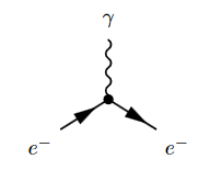
where the solid lines correspond to the electron, and the wiggly line to the photon. The corresponding product of distributions (prop. ) is (written in generalized function-notation, example )
Hence a typical Feynman diagram in the QED Feynman perturbation series induced by this electron-photon interaction looks as follows:
where on the bottom the corresponding Feynman amplitude product of distributions is shown; now notationally suppressing the contraction of the internal indices and all prefactors.
For instance the two solid edges between the vertices and correspond to the two factors of :
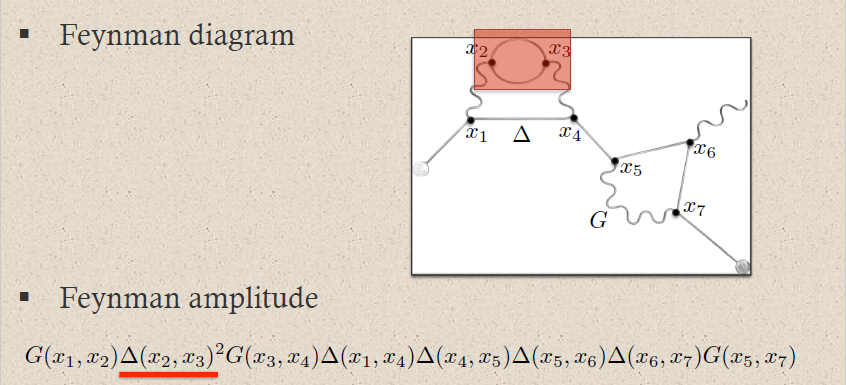
This way each sub-graph encodes its corresponding subset of factors in the Feynman amplitude:
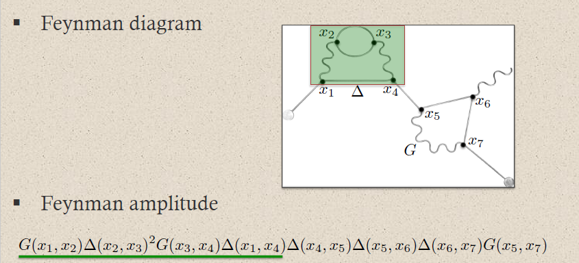
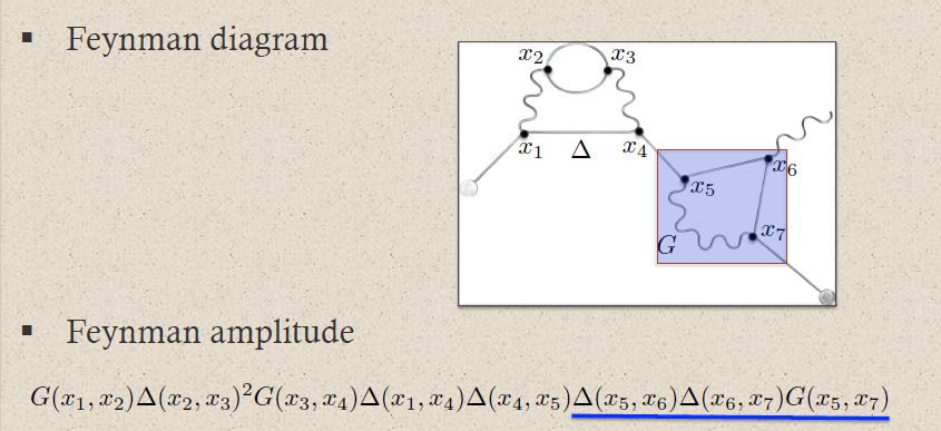
graphics grabbed from Brouder 10
A priori this product of distributions is defined away from coincident vertices: (prop. below). The definition at coincident vertices requires a choice of extension of distributions (def. below) to the diagonal locus of coincident interaction points. This choice is the ("re-")normalization (def. below) of the Feynman amplitude.
Example
Let be a relativistic free vacuum according to def. , and let
be a local observable, regarded as a adiabatically switched interaction action functional.
By prop. every choice of perturbative S-matrix (def. )
has an expansion as a formal power series of the form
where the series is over all finite multigraphs with linearly ordered vertices (def. ), and the summands are the corresponding ("re"-)normalized (def. ) Feynman amplitudes (prop. ).
If moreover a choice of field species and of internal and external interaction vertices is made, according to def. , then this series expansion refines to an expansion over all Feynman diagrams (def. ) of Feynman amplitudes (def. ):
Expressed in this form the S-matrix is known as the Feynman perturbation series.
Remark
(no tadpole Feynman diagrams)
In the definition of finite multigraphs in def. there are no edges considered that go from any vertex to itself. Accordingly, there are no such labeled edges in Feynman diagrams (def. ):

In pQFT these diagrams are called tadpoles, and their non-appearance is considered part of the Feynman rules (prop. ). Via prop. this condition reflects the nature of the star product (def. ) which always contracts different tensor product factors with the Feynman propagator before taking their pointwise product.
Beware that in graph theory these tadpoles are called “loops”, while here in pQFT a “loop” in a planar graph refers instead to what in graph theory is called a face of the graph, see the discussion of loop order in prop. below.
(Keller 10, remark II.8 and proof of prop. II.7)
Effective action
We have seen that the Feynman perturbation series expresses the S-matrix as a formal power series of Feynman amplitudes labeled by Feynman diagrams. Now the Feynman amplitude associated with a disjoint union of connected Feynman diagrams (def. below) is just the product of the amplitudes of the connected components (prop. below). This allows to re-organize the Feynman perturbation series as the ordinary exponential of the Feynman perturbation series restricted to just connected Feynman diagrams. The latter is called the effective action (def. below) because it allows to express vacuum expectation values of the S-matrix as an ordinary exponential (equation (248) below).
Definition
Given two finite multigraphs (def. ), their disjoint union
is the finite multigraph whose set of vertices and set of edges are the disjoint unions of the corresponding sets of and
and whose vertex-assigning function is the corresponding function on disjoint unions
The operation induces a pairing on the set of isomorphism classes of finite multigraphs
A finite multigraph (def. ) is called connected if it is not the disjoint union of two non-empty finite multigraphs.
We write
for the subset of isomorphism classes of connected finite multigraphs.
Lemma
(Feynman amplitudes multiply under disjoint union of graphs)
Let
be disjoint union of graphs (def. ). then then corresponding Feynman amplitudes (prop. ) multiply by the pointwise product (def. ):
Proof
By prop. the contributions to the S-matrix away from coinciding interaction points are given by the star product induced by the Feynman propagator, and specifically, by prop. , the Feynman amplitudes are given this way. Moreover the star product (def. ) is given by first contracting with powers of the Feynman propagator and then multiplying all resulting terms with the pointwise product of observables. This implies the claim by the nature of the combinatorial factor in the definition of the Feynman amplitudes (prop. ).
Definition
Let be a relativistic free vacuum according to def. , let be an S-matrix scheme for perturbative QFT around this vacuum (def. ) and let
be a local observable.
Recall that for each finite multigraph (def. ) the Feynman perturbation series for (example )
contributes with a ("re"-)nromalized Feynman amplitude .
We say that the corresponding effective action is times the sub-series
of Feynman amplitudes that are labeled only by the connected graphs (def. ).
(A priori could contain negative powers of , but it turns out that it does not; this is prop. below.)
Remark
(terminology for “effective action”)
Beware differing conventions of terminology:
-
In the perspective of effective quantum field theory (remark below), the effective action in def. is sometimes called the effective potential at scale (see prop. below).
This terminology originates in restriction to the special example of the scalar field (example ), where the non-derivative Phi^n interactions (example ) are naturally thought of as potential energy-terms.
From this perspective the effective action in def. is a special case of relative effective actions (“relative effective potentials”, in the case of Phi^n interactions) relative to an arbitrary UV cutoff-scales (def. below).
-
For the special case that
is a regular linear observable (def. ) the effective action according to def. is often denoted or , and then its functional Legendre transform (if that makes sense) is instead called the effective action, instead.
This is because the latter encodes the equations of motion for the vacuum expectation values of the interacting field observables; see example below.
Notice the different meaning of “effective” in both cases: In the first case it refers to what is effectively seen of the full pQFT at some UV-cutoff scale, while in the second case it refers to what is effectively seen when restricting attention only to the vacuum expectation values of regular linear observables.
Proposition
(effective action is logarithm of S-matrix)
Let be a relativistic free vacuum according to def. , let be an S-matrix scheme for perturbative QFT around this vacuum (def. ) and let
be a local observable and let
be the corresponding effective action (def. ).
Then then S-matrix for is the exponential of the effective action with respect to the pointwise product of observables (def. ):
Moreover, this relation passes to the vacuum expectation values:
Conversely the vacuum expectation value of the effective action is to the logarithm of that of the S-matrix:
Proof
By lemma the summands in the th pointwise power of times the effective action are precisely the Feynman amplitudes of finite multigraphs with connected components, where each such appears with multiplicity given by the factorial of :
It follows that
yields the Feynman perturbation series by expressing it as a series (re-)organized by number of connected components of the Feynman diagrams.
To conclude the proof it is now sufficient to observe that taking vacuum expectation values of polynomial observables respects the pointwise product of observables
This is because the Hadamard vacuum state simply picks the zero-order monomial term, by prop. ), and under multiplication of polynomials the zero-order terms are multiplied.
This immediately implies the following important fact:
Proposition
(in stable vacuum the effective action is generating function for vacuum expectation values of interacting field observables)
Let be a relativistic free vacuum according to def. , and let be a local observable regarded as an adiabatically switched interaction action functional.
If the given vacuum state is stable (def. ) then the vacuum expectation value of the effective action (def. ) is the generating function for the vacuum expectation value of the interacting field observable (def. ) in that
Proof
We compute as follows:
Here in the first step we used prop , in the second step we applied the chain rule of differentiation, in the third step we used the definition of vacuum stability (def. ) and in the fourth step we recognized the definition of the interacting field observables (def. ).
Example
(equations of motion for vacuum expectation values of interacting field observables)
Consider the effective action (def. ) for the case that
is a regular linear observable (this def.), hence the smearing of a field observable (this def.) by an adiabatic switching of the source field
(Here we are notationally suppressing internal field indices, for convenience.)
In this case the vacuum expectation value of the corresponding effective action is often denoted
and regarded as a functional of the adiabatic switching of the source field.
In this case prop. says that if the vacuum state is stable, then is the generating functional for interacting (def. ) field observables (def. ) in that
Assume then that there exists a corresponding functional of the field histories (def. ), which behaves like a functional Legendre transform of in that it satisfies the functional version of the defining equation of Legendre transforms (first derivatives are inverse functions of each other, see this equation):
By (249) this implies that
This may be read as a quantum version of the principle of extremal action (prop. ) formulated now not for the field histories , but for the vacuum expectation values of their corresponding interacting quantum field observables.
Beware, (as in remark ) that many texts refer to as the effective action, instead of its Legendre transform, the generating functional .
The perspective of the effective action gives a transparent picture of the order of quantum effects involved in the S-matrix, this is prop. below. In order to state this conveniently, we invoke two basic concepts from graph theory:
Definition
(planar graphs and trees)
A finite multigraph (def. ) is called a planar graph if it admits an embedding into the plane, hence if it may be “drawn into the plane” without intersections, in the evident way.
A finite multigraph is called a tree if for any two of its vertices there is at most one path of edges connecting them, these are examples of planar graphs. We write
for the subset of isomorphism classes of finite multigraphs with linearly orrdered vertices (def. ) on those which are trees.
Proposition
(loop order and tree level of Feynman perturbation series)
The effective action (def. ) contains no negative powers of , hence is indeed a formal power series also in :
and in particular
Moreover, the contribution to the effective action in the classical limit is precisely that of Feynman amplitudes of those finite multigraphs (prop. ) which are trees (def. ); thus called the tree level-contribution:
Finally, a finite multigraph (def. ) which is planar (def. ) and connected (def. ) contributes to the effective action precisely at order
where is the number of faces of , here called the number of loops of the diagram; here usually called the loop order of .
(Beware the terminology clash with graph theory, see the discussion of tadpoles in remark .)
Proof
By def. the explicit -dependence of the S-matrix is
and by prop. the further -dependence of the time-ordered product is
By the Feynman rules (prop. ) this means that
-
each vertex of a Feynman diagram contributes a power to its Feynman amplitude;
-
each edge of a Feynman diagram contributes a power to its Feynman amplitude.
If we write
for the total number of vertices and edges, respectively, in , this means that a Feynman amplitude corresponding to some contributes precisely at order
So far this holds for arbitrary . If however is connected (def. ) and planar (def. ), then Euler's formula asserts that
Hence is the order of at which contributes to the scattering matrix expressed as the Feynman perturbation series.
But the effective action, by definition (247), has the same contributions of Feynman amplitudes, but multiplied by another power of , hence it contributes at order
This proves the second claim on loop order.
The first claim, due to the extra factor of in the definition of the effective action, is equivalent to saying that the Feynman amplitude of every connected finite multigraph contributes powers in of order and contributes at order precisely if the graph is a tree.
Observe that a connected finite multigraph with vertices (necessarily ) has at least edges and precisely edges if it is a tree.
To see this, consecutively remove edges from as long as possible while retaining connectivity. When this process stops, the result must be a connected tree , hence a connected planar graph with . Therefore Euler's formula (251) implies that that .
This means that the connected multigraph in general has a Feynman amplitude of order
and precisely if it is a tree its Feynman amplitude is of order .
Vacuum diagrams
With the Feynman perturbation series and the effective action in hand, it is now immediate to see that there is a general contribution by vacuum diagrams (def. below) in the scattering matrix which, in a stable vacuum state, cancels out against the prefactor in Bogoliubov's formula for interacting field observables.
Definition
Let be a relativistic free vacuum according to def. , and let be a local observable regarded as an adiabatically switched interaction action functional, and consider a choice of decomposition for field species and interaction vertices according to def. .
Then a Feynman diagram all whose vertices are internal vertices (def. ) is called a vacuum diagram.
Write
for the subset of isomorphism classes of vacuum diagrams among the set of isomorphism classes of all Feynman diagrams, def. . Similarly write
for the subset of isomorphism classes of Feynman diagrams which are both vacuum diagrams as well as connected graphs (def. ).
Finally write
for the sub-series of that for the effective action (def. ) given only by those connected diagrams which are also vacuum diagrams.
Example
(2-vertex vacuum diagram in QED)
The vacuum diagram (def. ) with two electron-photon interaction-vertices in quantum electrodynamics (example ) is:
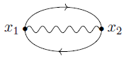
Example
(vacuum diagram-contribution to S-matrices)
Let be a relativistic free vacuum according to def. , and let be a local observable regarded as an adiabatically switched interaction action functional, and consider a choice of decomposition for field species and interaction vertices according to def. .
Then the Feynman perturbation series-expansion of the S-matrix (example ) of the interaction-term alone (no source field-contribution) is the series of Feynman amplitudes that are labeled by vacuum diagrams (def. ), hence (by prop. ) the exponential of the vacuum effective action (def. ):
More generally, the S-matrix with source field-contribution included always splits as a pointwise product of the vacuum S_matrix with the Feynman perturbation series over all Feynman graphs with at least one external vertex:
Hence if the free field vacuum state is stable with respect to the interaction , according to def. , then the vacuum expectation value of a time-ordered product of interacting field observables (example ) and hence in particular of scattering amplitudes (example ) is given by the Feynman perturbation series (example ) over just the non-vacuum Feynman diagrams, hence over all those diagram that have at least one one external vertex
This is the way in which the Feynman perturbation series is used in practice for computing scattering amplitudes.
Interacting quantum BV-Differential
So far we have discussed, starting with a BV-BRST gauge fixed free field vacuum, the perturbative construction of interacting field algebras of observables (def. ) and their organization in increasing powers of and (loop order, prop. ) via the Feynman perturbation series (example , example ).
But this interacting field algebra of observables still involves all the auxiliary fields of the BV-BRST gauge fixed free field vacuum (example ), while the actual physical gauge invariant on-shell observables should be (just) the cochain cohomology of the BV-BRST differential on this enlarged space of observables. Hence for the construction of perturbative QFT to conclude, it remains to pass the BV-BRST differential of the free field Wick algebra of observables to a differential on the interacting field algebra, such that its cochain cohomology is well defined.
Since the time-ordered products away from coinciding interaction points and as well as on regular polynomial observables are uniquely fixed (prop. ), one finds that also this interacting quantum BV-differential is uniquely fixed, on regular polynomial observables, by conjugation with the quantum Møller operators (def. ). The formula that characterizes it there is called the quantum master equation or equivalently the quantum master Ward identity (prop. below).
When extending to coinciding interaction points via ("re"-)normalization (def. ) these identities are not guaranteed to hold anymore, but may be imposed as renormalization conditions (def. , prop. ). Quantum correction to the master Ward identity then imply corrections to Noether current conservation laws; this we discuss below.
For the following discussion, recall from the previous chapter how the global BV-differential
on regular polynomial observables (def. ) as well as the global antibracket (def. ) are conjugated into the time-ordered product via the time ordering operator (def. , prop. ), which makes
In the same way we may use the quantum Møller operators to conjugate the BV-differential into the regular part of the interacting field algebra of observables:
Definition
(interacting quantum BV-differential)
Let be a relativistic free vacuum according to def. and let
be a regular polynomial observables, regarded as an adiabatically switched non-point-interaction action functional.
Then the interacting quantum BV-differential on the interacting field algebra on regular polynomial observables (def. ) is the conjugation of the plain global BV-differential (def. ) by the quantum Møller operator induced by (def. ):
Proposition
(quantum master equation and quantum master Ward identity on regular polynomial observables)
Consider an adiabatically switched non-point-interaction action functional in the form of a regular polynomial observable in degree 0
Then the following are equivalent:
-
The quantum master equation (QME)
(252) -
The perturbative S-matrix (def. ) is -closed
-
The quantum master Ward identity (MWI) on regular polynomial observables in terms of retarded products:
(253)expressing the interacting quantum BV-differential (def. ) as the sum of the time-ordered antibracket (def. ) with the total action functional and times the BV-operator (BV-operator).
-
The quantum master Ward identity (MWI) on regular polynomial observables in terms of time-ordered products:
(254)
(Rejzner 11, (5.35) - (5.38), following Hollands 07, (342)-(345))
Proof
To see that the first two conditions are equivalent, we compute as follows
Here in the first step we used the definition of the BV-operator (def. ) to rewrite the plain antibracket in terms of the time-ordered antibracket (def. ), then under the second brace we used that the time-ordered antibracket is the failure of the BV-operator to be a derivation (prop. ) and under the first brace the consequence of this statement for application to exponentials (example ). Finally we collected terms, and to “complete the square” we added the terms on the left of
which vanish because, by definition of gauge fixing (def. ), the free gauge-fixed action functional is independent of antifields.
But since the operation has the inverse , this implies the claim.
Next we show that the quantum master equation implies the quantum master Ward identities.
We use that the BV-differential is a derivation of the Wick algebra product (lemma ).
First of all this implies that with also .
Thus we compute as follows:
By applying to both sides of this equation, this means first of all that the interacting quantum BV-differential is equivalently given by
hence that if either version (253) or (257) of the master Ward identity holds, it implies the other.
Now expanding out the definition of (def. ) and expressing via the time-ordered antibracket (def. ) and the BV-operator (prop. ) as
(on regular polynomial observables), we continue computing as follows:
Here in the line with the braces we used that the BV-operator is a derivation of the time-ordered product up to correction by the time-ordered antibracket (prop. ), and under the first brace we used the effect of that property on time-ordered exponentials (example ), while under the second brace we used that is a derivation of the time-ordered product. Finally we have collected terms, added as before, and then used the QME.
This shows that the quantum master Ward identities follow from the quantum master equation. To conclude, it is now sufficient to show that, conversely, the MWI in terms of, say, retarded products implies the QME.
To see this, observe that with the BV-differential being nilpotent, also its conjugation by is, so that with the above we have:
Here under the brace we computed as follows:
where, in turn, the term under the first brace follows by the graded Jacobi identity, the one under the second brace by Henneaux-Teitelboim (15.105c) and the one under the third brace by Henneaux-Teitelboim (15.105b).
The quantum master Ward identity (prop. ) expresses the relation between the quantum (measured by Planck's constant ) interacting (measured by the coupling constant ) equations of motion to the classical free field equations of motion at (remark below). As such it generalizes the Schwinger-Dyson equation (prop. ), to which it reduces for (example below) as well as the classical master Ward identity, which is the case for (example below).
Applied to products of the equations of motion with any given observable, the master Ward identity becomes a particular Ward identity.
This is of interest notably in view of Noether's theorem (prop. ), which says that every infinitesimal symmetry of the Lagrangian of, in particular, the given free field theory, corresponds to a conserved current (def. ), hence a horizontal differential form whose total spacetime derivative vanishes up to a term proportional to the equations of motion. Under transgression to local observables this is a relation of the form
where “on shell” means up to the ideal generated by the classical free equations of motion. Hence for the case of local observables of the form , the quantum Ward identity expresses the possible failure of the original conserved current to actually be conserved, due to both quantum effects () and interactions (). This is the form in which Ward identities are usually understood (example below).
As one extends the time-ordered products to coinciding interaction points in ("re"-)normalization of the perturbative QFT (def. ), the quantum master equation/master Ward identity becomes a renormalization condition (def. , prop. ). If this condition fails, one speaks of a quantum anomaly. Specifically if the Ward identity for an infinitesimal gauge symmetry is violated, one speaks of a gauge anomaly.
Definition
Consider a free gauge fixed Lagrangian field theory (def. ) with global BV-differential on regular polynomial observables
Let moreover
be a regular polynomial observable (regarded as an adiabatically switched non-point-interaction action functional) such that the total action satisfies the quantum master equation (prop. ); and write
for the corresponding quantum Møller operator (def. ).
This is the quantum master Ward identity on regular polynomial observables, i.e. before renormalization.
Remark
(quantum master Ward identity relates quantum interacting field EOMs to classical free field EOMs)
For the quantum master Ward identity on regular polynomial observables (257) reads
The term on the right is manifestly in the image of the global BV-differential of the free field theory (def. ) and hence vanishes when passing to on-shell observables along the isomorphism (198)
Hence
In contrast, the left hand side is the interacting field observable (via def. ) of the sum of the time-ordered antibracket with the action functional of the interacting field theory and a quantum correction given by the BV-operator. If we use the definition of the BV-operator (def. ) we may equivalently re-write this as
Hence the quantum master Ward identity expresses a relation between the ideal spanned by the classical free field equations of motion and the quantum interacting field equations of motion.
Example
(free field-limit of master Ward identity is Schwinger-Dyson equation)
In the free field-limit (noticing that in this limit ) the quantum master Ward identity (257) reduces to
which is the defining equation for the BV-operator (221), hence is isomorphic (under ) to the Schwinger-Dyson equation (prop. )
Example
(classical limit of quantum master Ward identity)
In the classical limit (noticing that the classical limit of is ) the quantum master Ward identity (257) reduces to
This says that the interacting field observable corresponding to the global antibracket with the action functional of the interacting field theory vanishes on-shell, classically.
Applied to an observable which is linear in the antifields
this yields
This is the classical master Ward identity according to (Dütsch-Fredenhagen 02, Brennecke-Dütsch 07, (5.5)), following (Dütsch-Boas 02).
Example
(quantum correction to Noether current conservation)
Let be an evolutionary vector field, which is an infinitesimal symmetry of the Lagrangian , and let the corresponding conserved current, by Noether's theorem I (prop. ), so that
by (80), where in the second line we just rewrote the expression in components (50)
and re-arranged suggestively.
Then for any choice of bump function, we obtain the local observables
and
by transgression of variational differential forms.
This is such that
Hence applied to this choice of local observable , the quantum master Ward identity (259) now says that
Hence the interacting field observable-version of need not vanish itself on-shell, instead there may be a correction as shown on the right.
This concludes our discussion of perturbative quantum observables of interacting field theories. In the next chapter wé discuss explicitly the inductive construction via ("re"-)normalization of time-ordered products/Feynman amplitudes as well as the various incarnations of the re-normalization group passing between different choices of such ("re"-)normalizations.
Renormalization
In this chapter we discuss the following topics:
In the previous chapter we have seen that the construction of interacting perturbative quantum field theories is given by perturbative S-matrix schemes (def. ), equivalently by time-ordered products (def. ) or equivalently by Feynman amplitudes (prop. ). These are uniquely fixed away from coinciding interaction points (prop. ) by the given local interaction (prop. ), but involve further choices of interactions whenever interaction vertices coincide (prop. ). This choice is called the choice of ("re"-)normalization (def. ) in perturbative QFT.
In this rigorous discussion no “infinite divergent quantities” (as in the original informal discussion due to Schwinger-Tomonaga-Feynman-Dyson) that need to be “re-normalized” to finite well-defined quantities are ever considered, instead finite well-defined quantities are considered right away, and the available space of choices is determined. Therefore making such choices is rather a normalization of the time-ordered products/Feynman amplitudes (as prominently highlighted in Scharf 95, see title, introduction, and section 4.3). Actual re-normalization is the the change of such normalizations.
The construction of perturbative QFTs may be explicitly described by an inductive extension of distributions of time-ordered products/Feynman amplitudes to coinciding interaction points. This is called
This inductive construction has the advantage that it gives accurate control over the space of available choices of (“re”-)normalizations (theorem below) but it leaves the nature of the “new interactions” that are to be chosen at coinciding interaction points somwewhat implicit.
Alternatively, one may re-define the interactions explicitly (by adding “counterterms”, remark below), depending on a chosen UV cutoff-scale (def. below), and construct the limit as the “cutoff is removed” (prop. below). This is called (“re”-)normalization by
This still leaves open the question how to choose the counterterms. For that it serves to understand the relative effective action induced by the choice of UV cutoff at any given cutoff scale (def. below). This is the perspective of effective quantum field theory (remark below).
The infinitesimal change of these relative effective actions follows a universal differential equation, known as Polchinski's flow equation (prop. below). This makes the problem of (“re”-)normalization be that of solving this differential equation subject to chosen initial data. This is the perspective on (“re”-)normalization called
The main theorem of perturbative renormalization (theorem below) states that different S-matrix schemes are precisely related by vertex redefinitions. This yields the
If a sub-collection of renormalization schemes is parameterized by some group , then the main theorem implies vertex redefinitions depending on pairs of elements of (prop. below). This is known as
Specifically scaling transformations on Minkowski spacetime yield such a collection of renormalization schemes (prop. below); the corresponding renormalization group flow is known as
The infinitesimal behaviour of this flow is known as the beta function, describing the running of the coupling constants with scale (def. below).
The construction of perturbative quantum field theories around a given gauge fixed relativistic free field vacuum is equivalently, by prop. , the construction of S-matrices in the sense of causal perturbation theory (def. ) for the given local interaction . By prop. the construction of these S-matrices is inductively in a choice of extension of distributions (remark and def. below) of the corresponding -ary time-ordered products of the interaction to the locus of coinciding interaction points. An inductive construction of the S-matrix this way is called Epstein-Glaser-("re"-)normalization (def. ).
By paying attention to the scaling degree (def. below) one may precisely characterize the space of choices in the extension of distributions (prop. below): For a given local interaction it is inductively in a finite-dimensional affine space. This conclusion is theorem below.
Proposition
(("re"-)normalization is inductive extension of time-ordered products to diagonal)
Let be a gauge-fixed relativistic free vacuum according to def. ).
Assume that for , time-ordered products of arity have been constructed in the sense of def. . Then the time-ordered product of arity is uniquely fixed on the complement
of the image of the diagonal inclusion (where we regarded as a generalized function on according to remark ).
This statement appears in (Popineau-Stora 82), with (unpublished) details in (Stora 93), following personal communication by Henri Epstein (according to Dütsch 18, footnote 57). Following this, statement and detailed proof appeared in (Brunetti-Fredenhagen 99).
Proof
We will construct an open cover of by subsets which are disjoint unions of non-empty sets that are in causal order, so that by causal factorization the time-ordered products on these subsets are uniquely given by . Then we show that these unique products on these special subsets do coincide on intersections. This yields the claim by a partition of unity.
We now say this in detail:
For write . For , define the subset
Since the causal order-relation involves the closed future cones/closed past cones, respectively, it is clear that these are open subsets. Moreover it is immediate that they form an open cover of the complement of the diagonal:
(Because any two distinct points in the globally hyperbolic spacetime may be causally separated by a Cauchy surface, and any such may be deformed a little such as not to intersect any of a given finite set of points. )
Hence the condition of causal factorization on implies that restricted to any these have to be given (in the condensed generalized function-notation from remark ) on any unordered tuple with corresponding induced tuples and by
This shows that is unique on if it exists at all, hence if these local identifications glue to a global definition of . To see that this is the case, we have to consider any two such subsets
By definition this implies that for
a tuple of spacetime points which decomposes into causal order with respect to both these subsets, the corresponding mixed intersections of tuples are spacelike separated:
By the assumption that the satisfy causal factorization, this implies that the corresponding time-ordered products commute:
Using this we find that the identifications of on and on , accrding to (260), agree on the intersection: in that for we have
Here in the first step we expanded out the two factors using (260) for , then under the brace we used (261) and in the last step we used again (260), but now for .
To conclude, let
be a partition of unity subordinate to the open cover formed by the :
Then the above implies that setting for any
is well defined and satisfies causal factorization.
Remark
(time-ordered products of fixed interaction as distributions)
Let be a gauge-fixed relativistic free vacuum according to def. , and assume that the field bundle is a trivial vector bundle (example )
and let
be a polynomial local observable as in def. , to be regarded as a adiabatically switched interaction action functional. This means that there is a finite set
of Lagrangian densities which are monomials in the field and jet coordinates, and a corresponding finite set
of adiabatic switchings, such that
is the transgression of variational differential forms (def. ) of the sum of the products of these adiabatic switching with these Lagrangian densities.
In order to discuss the S-matrix and hence the time-ordered products of the special form it is sufficient to restrict attention to the restriction of each to the subspace of local observables induced by the finite set of Lagrangian densities .
This restriction is a continuous linear functional on the corresponding space of bump functions , hence a dstributional section of a corresponding trivial vector bundle.
In terms of this, prop. says that the choice of time-ordered products is inductively in a choice of extension of distributions to the diagonal.
If is Minkowski spacetime and we impose the renormalization condition “translation invariance” (def. ) then each is a distribution on and the extension of distributions is from the complement of the origina .
Therefore we now discuss extension of distributions (def. below) on Cartesian spaces from the complement of the origin to the origin. Since the space of choices of such extensions turns out to depend on the scaling degree of distributions, we first discuss that (def. below).
Definition
Let . For a positive real number write
for the diffeomorphism given by multiplication with , using the canonical real vector space-structure of .
Then for a distribution on the Cartesian space the rescaled distribution is the pullback of along
Explicitly, this is given by
Similarly for an open subset which is invariant under , the rescaling of a distribution is is .
Definition
(scaling degree of a distribution)
Let and let be an open subset of Cartesian space which is invariant under rescaling (def. ) for all , and let be a distribution on this subset. Then
-
The scaling degree of is the infimum
of the set of real numbers such that the limit of the rescaled distribution (def. ) vanishes. If there is no such one sets .
-
The degree of divergence of is the difference of the scaling degree by the dimension of the underlying space:
Example
(scaling degree of non-singular distributions)
If is a non-singular distribution given by bump function , then its scaling degree (def. ) is non-positive
Specifically if the first non-vanishing partial derivative of at 0 occurs at order , then the scaling degree of is .
Proof
By definition we have for any bump function that
where in last line we applied change of integration variables.
The limit of this expression is clearly zero for all , which shows the first claim.
If moreover the first non-vanishing partial derivative of occurs at order , then Hadamard's lemma says that is of the form
where the are smooth functions. Hence in this case
This makes manifest that the expression goes to zero with precisely for , which means that
in this case.
Example
(scaling degree of derivatives of delta-distributions)
Let be a multi-index and the corresponding partial derivatives of the delta distribution supported at . Then the degree of divergence (def. ) of is the total order the derivatives
where .
Proof
By definition we have for any bump function that
where in the last step we used the chain rule of differentiation. It is clear that this goes to zero with as long as . Hence .
Example
(scaling degree of Feynman propagator on Minkowski spacetime)
Let
be the Feynman propagator for the massive free real scalar field on -dimensional Minkowski spacetime (prop. ). Its scaling degree is
(Brunetti-Fredenhagen 00, example 3 on p. 22)
Proof
Regarding as a generalized function via the given Fourier-transform expression, we find by change of integration variables in the Fourier integral that in the scaling limit the Feynman propagator becomes that for vannishing mass, which scales homogeneously:
Proposition
(basic properties of scaling degree of distributions)
Let and be a distribution as in def. , such that its scaling degree is finite: (def. ). Then
-
For , the partial derivative of distributions increases scaling degree at most by :
-
For , the product of distributions with the smooth coordinate functions decreases scaling degree at least by :
-
Under tensor product of distributions their scaling degrees add:
for another distribution on ;
-
for and for ;
(Brunetti-Fredenhagen 00, lemma 5.1, Dütsch 18, exercise 3.34)
Proof
The first three statements follow with manipulations as in example and example .
For the fourth…
Proposition
(scaling degree of product distribution)
Let be two distributions such that
-
both have finite degree of divergence (def. )
-
their product of distributions is well-defined
(in that their wave front sets satisfy Hörmander's criterion)
then the product distribution has degree of divergence bounded by the sum of the separate degrees:
With the concept of scaling degree of distributions in hand, we may now discuss extension of distributions:
Definition
Let be an inclusion of open subsets of some Cartesian space. This induces the operation of restriction of distributions
Given a distribution , then an extension of to is a distribution such that
Proposition
(unique extension of distributions with negative degree of divergence)
For , let be a distribution on the complement of the origin, with negative degree of divergence at the origin
Then has a unique extension of distributions to the origin with the same degree of divergence
(Brunetti-Fredenhagen 00, theorem 5.2, Dütsch 18, theorem 3.35 a))
Proof
Regarding uniqueness:
Suppose and are two extensions of with . Both being extensions of a distribution defined on , this difference has support at the origin . By prop. this implies that it is a linear combination of derivatives of the delta distribution supported at the origin:
for constants . But by example the degree of divergence of these point-supported distributions is non-negative
This implies that for all , hence that the two extensions coincide.
Regarding existence:
Let
be a bump function which is and constant on 1 over a neighbourhood of the origin. Write
graphics grabbed from Dütsch 18, p. 108
and for a positive real number, write
Since the product has support of a distribution on a complement of a neighbourhood of the origin, we may extend it by zero to a distribution on all of , which we will denote by the same symbols:
By construction coincides with away from a neighbourhood of the origin, which moreover becomes arbitrarily small as increases. This means that if the following limit exists
then it is an extension of .
To see that the limit exists, it is sufficient to observe that we have a Cauchy sequence, hence that for all the difference
becomes arbitrarily small.
It remains to see that the unique extension thus established has the same scaling degree as . This is shown in (Brunetti-Fredenhagen 00, p. 24).
Proposition
(space of point-extensions of distributions)
For , let be a distribution of degree of divergence .
Then does admit at least one extension (def. ) to a distribution , and every choice of extension has the same degree of divergence as
Moreover, any two such extensions and differ by a linear combination of partial derivatives of distributions of order of the delta distribution supported at the origin:
for a finite number of constants .
This is essentially (Hörmander 90, thm. 3.2.4). We follow (Brunetti-Fredenhagen 00, theorem 5.3), which was inspired by (Epstein-Glaser 73, section 5). Review of this approach is in (Dütsch 18, theorem 3.35 (b)), see also remark below.
Proof
For a smooth function, and , we say that vanishes to order at the origin if all partial derivatives with multi-index of total order vanish at the origin:
By Hadamard's lemma, such a function may be written in the form
for smooth functions .
Write
for the subspace of that of all bump functions on those that vanish to order at the origin.
By definition this is equivalently the joint kernel of the partial derivatives of distributions of order of the delta distribution supported at the origin:
Therefore every continuous linear projection
may be obtained from a choice of dual basis to the , hence a choice of smooth functions
such that
by setting
hence
Together with Hadamard's lemma in the form (264) this means that every is decomposed as
Now let
Observe that (by prop. ) the degree of divergence of the product of distributions with is negative
Therefore prop. says that each for has a unique extension to the origin. Accordingly the composition has a unique extension, by (267):
That says that is of the form
for a finite number of constants .
Notice that for any extension the exact value of the here depends on the arbitrary choice of dual basis used for this construction. But the uniqueness of the first summand means that for any two choices of extensions and , their difference is of the form
where the constants are independent of any choices.
It remains to see that all these in fact have the same degree of divergence as .
By example the degree of divergence of the point-supported distributions on the right is .
Therefore to conclude it is now sufficient to show that
This is shown in (Brunetti-Fredenhagen 00, p. 25).
Remark
(“W-extensions”)
Since in Brunetti-Fredenhagen 00, (38) the projectors (266) are denoted “”, the construction of extensions of distributions via the proof of prop. has come to be called “W-extensions” (e.g Dütsch 18).
In conclusion we obtain the central theorem of causal perturbation theory:
Theorem
(existence and choices of ("re"-)normalization of S-matrices/perturbative QFTs)
Let be a gauge-fixed relativistic free vacuum, according to def. , such that the underlying spacetime is Minkowski spacetime and the Wightman propagator is translation-invariant.
Then:
-
an S-matrix scheme (def. ) around this vacuum exists;
-
for a local observable as in def. , regarded as an adiabatically switched interaction action functional, the space of possible choices of S-matrices
hence of the corresponding perturbative QFTs, by prop. , is, inductively in , a finite dimensional affine space, parameterizing the extension of the time-ordered product to the locus of coinciding interaction points.
Proof
By prop. the Feynman propagator is finite scaling degree of a distribution, so that by prop. the binary time-ordered product away from the diagonal has finite scaling degree.
By prop. this implies that in the inductive description of the time-ordered products by prop. , each induction step is the extension of distributions of finite scaling degree of a distribution to the point. By prop. this always exists.
This proves the first statement.
Now if a polynomial local interaction is fixed, then via remark each induction step involved extending a finite number of distributions, each of finite scaling degree. By prop. the corresponding space of choices is in each step a finite-dimensional affine space.
Stückelberg-Petermann renormalization group
A genuine re-normalization is the passage from one S-matrix ("re"-)normalization scheme to another such scheme . The inductive Epstein-Glaser ("re"-normalization) construction (prop. ) shows that the difference between any and is inductively in a choice of extra term in the time-ordered product of factors, equivalently in the Feynman amplitudes for Feynman diagrams with vertices, that contributes when all of these vertices coincide in spacetime (prop. ).
A natural question is whether these additional interactions that appear when several interaction vertices coincide may be absorbed into a re-definition of the original interaction . Such an interaction vertex redefinition (def. below)
should perturbatively send local interactions to local interactions with higher order corrections.
The main theorem of perturbative renormalization (theorem below) says that indeed under mild conditions every re-normalization is induced by such an interaction vertex redefinition in that there exists a unique such redefinition so that for every local interaction we have that scattering amplitudes for the interaction computed with the ("re"-)normalization scheme equal those computed with but applied to the re-defined interaction :
This means that the interaction vertex redefinitions form a group under composition which acts transitively and freely, hence regularly, on the set of S-matrix ("re"-)normalization schemes; this is called the Stückelberg-Petermann renormalization group (theorem below).
Definition
(perturbative interaction vertex redefinition)
Let be a gauge fixed free field vacuum (def. ).
A perturbative interaction vertex redefinition (or just vertex redefinition, for short) is an endofunction
on local observables with formal parameters adjoined (def. ) such that there exists a sequence of continuous linear functionals, symmetric in their arguments, of the form
such that for all the following conditions hold:
-
(perturbation)
-
and
-
(field independence) The local observable depends on the field histories only through its argument , hence by the chain rule:
(269)
The following proposition should be compared to the axiom of causal additivity of the S-matrix scheme (230):
Proposition
(local additivity of vertex redefinitions)
Let be a gauge fixed free field vacuum (def. ) and let be a vertex redefinition (def. ).
Then for all local observables with spacetime support denoted (def. ) we have
-
(local additivity)
-
(preservation of spacetime support)
hence in particular
Proof
Under the inclusion
of local observables into polynomial observables we may think of each as a generalized function, as for time-ordered products in remark .
Hence if
is the transgression of a Lagrangian density we get
Now by definition is in the subspace of local observables, i.e. those polynomial observables whose coefficient distributions are supported on the diagonal, which means that
Together with the axiom “field independence” (269) this means that the support of these generalized functions in the integrand here must be on the diagonal, where .
By the assumption that the spacetime supports of and are disjoint, this means that only the summands with and those with contribute to the above sum. Removing the overcounting of those summands where all we get
This directly implies the claim.
As a corollary we obtain:
Proposition
(composition of S-matrix scheme with vertex redefinition is again S-matrix scheme)
Let be a gauge fixed free field vacuum (def. ) and let be a vertex redefinition (def. ).
Then for
and S-matrix scheme (def. ), the composite
is again an S-matrix scheme.
Moreover, if satisfies the renormalization condition “field independence” (prop. ), then so does .
(e.g Dütsch 18, theorem 3.99 (b))
Proof
It is clear that causal order of the spacetime supports implies that they are in particular disjoint
Therefore the local additivity of (prop. ) and the causal factorization of the S-matrix (remark ) imply the causal factorization of the composite:
But by prop. this implies in turn causal additivity and hence that is itself an S-matrix scheme.
Finally that satisfies “field indepndence” if does is immediate by the chain rule, given that satisfies this condition by definition.
Proposition
(any two S-matrix renormalization schemes differ by unique vertex redefinition)
Let be a gauge fixed free field vacuum (def. ).
Then for any two S-matrix schemes (def. ) which both satisfy the renormalization condition “field independence”, the there exists a unique vertex redefinition (def. ) relating them by composition, i. e. such that
Proof
By applying both sides of the equation to linear combinations of local observables of the form and then taking derivatives with respect to at (as in example ) we get that the equation in question implies
which in components means that
where are the time-ordered products corresponding to (by example ) and those correspondong to .
Here the sum on the right runs over all ways that in the composite a -ary operation arises as the composite of an -ary time-ordered product applied to the -ary components of , for running from 1 to ; except for the case , which is displayed separately in the second line
This shows that if exists, then it is unique, because its coefficients are inductively in given by the expressions
(The symbol under the brace is introduced as a convenient shorthand for the term above the brace.)
Hence it remains to see that the defined this way satisfy the conditions in def. .
The condition “perturbation” is immediate from the corresponding condition on and .
Similarly the condition “field independence” follows immediately from the assumoption that and satisfy this condition.
It only remains to see that indeed takes values in local observables. Given that the time-ordered products a priori take values in the larrger space of microcausal polynomial observables this means to show that the spacetime support of is on the diagonal.
But observe that, as indicated in the above formula, the term over the brace may be understood as the coefficient at order of the exponential series-expansion of the composite , where
is the truncation of the vertex redefinition to degree . This truncation is clearly itself still a vertex redefinition (according to def. ) so that the composite is still an S-matrix scheme (by prop. ) so that the are time-ordered products (by example ).
So as we solve inductively in degree , then for the induction step in degree the expressions and agree and are both time-ordered products. By prop. this implies that and agree away from the diagonal. This means that their difference is supported on the diagonal, and hence is indeed local.
In conclusion this establishes the following pivotal statement of perturbative quantum field theory:
Theorem
(main theorem of perturbative renormalization – Stückelberg-Petermann renormalization group of vertex redefinitions)
Let be a gauge fixed free field vacuum (def. ).
-
the vertex redefinitions (def. ) form a group under composition;
-
the set of S-matrix ("re"-)normalization schemes (def. ), remark ) satisfying the renormalization condition “field independence” (prop. ) is a torsor over this group, hence equipped with a regular action in that
-
the set of S-matrix schemes is non-empty;
-
any two S-matrix ("re"-)normalization schemes , are related by a unique vertex redefinition via composition:
-
This group is called the Stückelberg-Petermann renormalization group.
Typically one imposes a set of renormalization conditions (def. ) and considers the corresponding subgroup of vertex redefinitions preserving these conditions.
Proof
The group-structure and regular action is given by prop. and prop. . The existence of S-matrices follows is the statement of Epstein-Glaser ("re"-)normalization in theorem .
UV-Regularization via counterterms
While Epstein-Glaser renormalization (prop. ) gives a transparent picture on the space of choices in ("re"-)normalization (theorem ) the physical nature of the higher interactions that it introduces at coincident interaction points (via the extensions of distributions in prop. ) remains more implicit. But the main theorem of perturbative renormalization (theorem ), which re-expresses the difference between any two such choices as an interaction vertex redefinition, suggests that already the choice of ("re"-)normalization itself should have an incarnation in terms of interaction vertex redefinitions.
This may be realized via a construction of ("re"-)normalization in terms of UV-regularization (prop. below): For any choice of “UV-cutoff”, given by an approximation of the Feynman propagator by non-singular distributions (def. below) there is a unique “effective S-matrix” induced at each cutoff scale (def. below). While the “UV-limit” does not in general exist, it may be “regularized” by applying suitable interaction vertex redefinitions ; if the higher-order corrections that these introduce serve to “counter” (remark below) the coresponding UV-divergences.
This perspective of ("re"-)normalization via via counterterms is often regarded as the primary one. Its elegant proof in prop. below, however relies on the Epstein-Glaser renormalization via inductive extensions of distributions and uses the same kind of argument as in the proof of the main theorem of perturbative renormalization (theorem via prop. ) that establishes the Stückelberg-Petermann renormalization group.
Definition
Let be a gauge fixed relativistic free vacuum over Minkowski spacetime (according to def. ), where is the corresponding Wightman propagator inducing the Feynman propagator
by .
Then a choice of UV cutoffs for perturbative QFT around this vacuum is a collection of non-singular distributions parameterized by positive real numbers
such that:
-
each satisfies the following basic properties
-
(translation invariance)
-
(symmetry)
i.e.
-
-
the interpolate between zero and the Feynman propagator, in that, in the Hörmander topology:
-
the limit as exists and is zero
-
the limit as exists and is the Feynman propagator:
-
Example
(relativistic momentum cutoff)
Recall from this prop. that the Fourier transform of distributions of the Feynman propagator for the real scalar field on Minkowski spacetime is,
To produce a UV cutoff in the sense of def. we would like to set this function to zero for wave numbers (hence momenta ) larger than a given .
This needs to be done with due care: First, the Paley-Wiener-Schwartz theorem (prop. ) says that to be a test function and hence compactly supported, its Fourier transform needs to be smooth and of bounded growth. So instead of multiplying by a step function in , we may multiply it with an exponential damping.
(Keller-Kopper-Schophaus 97, section 6.1, Dütsch 18, example 3.126)
Definition
Let be a gauge fixed relativistic free vacuum (according to def. ) and let be a choice of UV cutoffs for perturbative QFT around this vacuum (def. ).
We say that the effective S-matrix scheme at cutoff scale
is the exponential series
with respect to the star product induced by the (def. ).
This is evidently defined on all polynomial observables as shown, and restricts to an endomorphism on microcausal polynomial observables as shown, since the contraction coefficients are non-singular distributions, by definition of UV cutoff.
Proposition
(("re"-)normalization via UV regularization)
Let be a gauge fixed relativistic free vacuum (according to def. ) and let a polynomial local observable as in def. , regarded as an adiabatically switched interaction action functional.
Let moreover be a UV cutoff (def. ); with the induced effective S-matrix schemes (271).
Then
-
there exists a -parameterized interaction vertex redefinition (def. ) such that the limit of effective S-matrix schemes (271) applied to the -redefined interactions
exists and is a genuine S-matrix scheme around the given vacuum (def. );
-
every S-matrix scheme around the given vacuum arises this way.
These are called counterterms (remark below) and the composite is called a UV regularization of the effective S-matrices .
Hence UV-regularization via counterterms is a method of ("re"-)normalization of perturbative QFT (def. ).
This was claimed in (Brunetti-Dütsch-Fredenhagen 09, (75)), a proof was indicated in (Dütsch-Fredenhagen-Keller-Rejzner 14, theorem A.1).
Proof
Let be a sequence of projection maps as in (265) defining an Epstein-Glaser ("re"-)normalization (prop. ) of time-ordered products as extensions of distributions of the , regarded as distributions via remark , by the choice in (268).
We will construct that in terms of these projections .
First consider some convenient shorthand:
For , write . Moreover, for write for the -ary coefficient in the expansion of the composite , as in equation (270) in the proof of the main theorem of perturbative renormalization (theorem , via prop. ).
In this notation we need to find such that for each we have
We proceed by induction over .
Since by definition , and , the statement is trivially true for and .
So assume now and has been found such that (272) holds.
Observe that with the chosen renormalizing projection the time-ordered product may be expressed as follows:
Here in the first step we inserted the causal decomposition (263) of in terms of the away from the diagonal, as in the proof of prop. , which is admissible because the image of vanishes on the diagonal. In the second step we replaced the star-product of the Feynman propagator with the limit over the star-products of the regularized propagators , which converges by the nature of the Hörmander topology (which is assumed by def. ).
Hence it is sufficient to find and such that
subject to these two conditions:
-
is local;
-
.
Now by expanding out the left hand side of (274) as
(which uses the condition ) we find the unique solution of (274) for , in terms of the and (the latter still to be chosen) to be:
We claim that the following choice works:
To prove this, we need to show that 1) the resulting is local and 2) the limit of vanishes as .
First regarding the locality of : By inserting (276) into (275) we obtain
By definition is the identity on test functions (adiabatic switchings) that vanish at the diagonal. This means that is supported on the diagonal, and is hence local.
Second we need to show that :
By applying the analogous causal decomposition (263) to the regularized products, we find
Using this we compute as follows:
Here in the first step we inserted (277); in the second step we used that in the Hörmander topology the product of distributions preserves limits in each variable and in the third step we used the induction assumption (272) and the definition of UV cutoff (def. ).
Inserting this for the first summand in (276) shows that .
In conclusion this shows that a consistent choice of counterterms exists to produce some S-matrix . It just remains to see that for every other S-matrix there exist counterterms such that .
But by the main theorem of perturbative renormalization (theorem ) we know that there exists a vertex redefinition such that
and hence with counterterms for given, then counterterms for any are given by the composite .
Remark
Let be a gauge fixed relativistic free vacuum (according to def. ) and let be a choice of UV cutoffs for perturbative QFT around this vacuum (def. ).
Consider
a local observable, regarded as an adiabatically switched interaction action functional.
Then prop. says that there exist vertex redefinitions of this interaction
parameterized by , such that the limit
exists and is an S-matrix for perturbative QFT with the given interaction .
In this case the difference
(which by the axiom “perturbation” in def. is at least of second order in the coupling constant/source field, as shown) is called a choice of counterterms at cutoff scale . These are new interactions which are added to the given interaction at cutoff scale
In this language prop. says that for every free field vacuum and every choice of local interaction, there is a choice of counterterms to the interaction that defines a corresponding ("re"-)normalized perturbative QFT, and every (re"-)normalized perturbative QFT arises from some choice of counterterms.
Wilson-Polchinski effective QFT flow
We have seen above that a choice of UV cutoff induces effective S-matrix schemes at cutoff scale (def. ). To these one may associated non-local relative effective actions (def. below) which are such that their effective scattering amplitudes at scale coincide with the true scattering amplitudes of a genuine local interaction as the cutoff is removed. This is the Wilsonian picture of effective quantum field theory at a given cutoff scale (remark below). Crucially the “flow” of the relative effective actions with the cutoff scale satisfies a differential equation that in itself is independent of the full UV-theory; this is Polchinski's flow equation (prop. below). Solving this equation for given choice of initial value data is hence another way of choosing ("re"-)normalization constants.
Proposition
(effective S-matrix schemes are invertible functions)
Let be a gauge fixed relativistic free vacuum (according to def. ) and let be a choice of UV cutoffs for perturbative QFT around this vacuum (def. ).
Write
for the subspace of the space of formal power series in with coefficients polynomial observables on those which are at least of first order in , i.e. those that vanish for (as in def. ).
Write moreover
for the subspace of polynomial observables which are the sum of 1 (the multiplicative unit) with an observable at least linear n .
Then the effective S-matrix schemes (def. ) restrict to linear isomorphisms of the form
Proof
Since each is symmetric (def. ) if follows by general properties of star products (prop. ) just as for the genuine time-ordered product on regular polynomial observables (prop. ) that eeach the “effective time-ordered product” is isomorphic to the pointwise product (def. )
for
as in (?).
In particular this means that the effective S-matrix arises from the exponential series for the pointwise product by conjugation with :
(just as for the genuine S-matrix on regular polynomial observables in def. ).
Now the exponential of the pointwise product on has as inverse function the natural logarithm power series, and since evidently preserves powers of this conjugates to an inverse at each UV cutoff scale :
Definition
Let be a gauge fixed relativistic free vacuum (according to def. ) and let be a choice of UV cutoffs for perturbative QFT around this vacuum (def. ).
Consider
a local observable regarded as an adiabatically switched interaction action functional.
Then for
two UV cutoff-scale parameters, we say the relative effective action is the image of this interaction under the composite of the effective S-matrix scheme at scale (271) and the inverse function of the effective S-matrix scheme at scale (via prop. ):
For chosen counterterms (remark ) hence for chosen UV regularization (prop. ) this makes sense also for and we write:
Remark
(effective quantum field theory)
Let be a gauge fixed relativistic free vacuum (according to def. ), let be a choice of UV cutoffs for perturbative QFT around this vacuum (def. ), and let be a corresponding UV regularization (prop. ).
Consider a local observable
regarded as an adiabatically switched interaction action functional.
Then def. and def. say that for any the effective S-matrix (271) of the relative effective action (280) equals the genuine S-matrix of the genuine interaction :
In other words the relative effective action encodes what the actual perturbative QFT defined by effectively looks like at UV cutoff .
Therefore one says that defines effective quantum field theory at UV cutoff .
Notice that in general is not a local interaction anymore: By prop. the image of the inverse of the effective S-matrix is microcausal polynomial observables in and there is no guarantee that this lands in the subspace of local observables.
Therefore effective quantum field theories at finite UV cutoff-scale are in general not local field theories, even if their limit as is, via prop. .
Proposition
(effective action is relative effective action at )
Let be a gauge fixed relativistic free vacuum (according to def. ) and let be a choice of UV cutoffs for perturbative QFT around this vacuum (def. ).
Then the relative effective action (def. ) at is the actual effective action (def. ) in the sense of the the Feynman perturbation series of Feynman amplitudes (def. ) for connected Feynman diagrams :
More generally this holds true for any
where denotes the evident version of the Feynman amplitude (def. ) with time-ordered products replaced by effective time ordered product at scale as in (def. ).
Proof
Observe that the effective S-matrix scheme at scale (271) is the exponential series with respect to the pointwise product (def. )
Therefore the statement to be proven says equivalently that the exponential series of the effective action with respect to the pointwise product is the S-matrix:
The definition of the relative effective action in def. invokes a choice of UV regularization (prop. ). While (by that proposition and the main theorem of perturbative renormalization, theorem )this is guaranteed to exist, in practice one is after methods for constructing this without specifying it a priori.
But the collection relative effective actions for “flows” with the cutoff-parameters and in particular also with (remark below) which suggests that examination of this flow yields information about full theory at .
This is made precise by Polchinski's flow equation (prop. below), which is the infinitesimal version of the “Wilsonian RG flow” (remark ). As a differential equation it is independent of the choice of and hence may be used to solve for the Wilsonian RG flow without knowing in advance.
The freedom in choosing the initial values of this differential equation corresponds to the ("re"-)normalization freedom in choosing the UV regularization . In this sense “Wilsonian RG flow” is a method of ("re"-)normalization of perturbative QFT (def. ).
Remark
(Wilsonian groupoid of effective quantum field theories)
Let be a gauge fixed relativistic free vacuum (according to def. ) and let be a choice of UV cutoffs for perturbative QFT around this vacuum (def. ).
Then the relative effective actions (def. ) satisfy
This is similar to a group of UV-cutoff scale-transformations. But since the composition operations are only sensible when the UV-cutoff labels match, as shown, it is really a groupoid action.
This is often called the Wilsonian RG.
We now consider the infinitesimal version of this “flow”:
Proposition
Let be a gauge fixed relativistic free vacuum (according to def. ), let be a choice of UV cutoffs for perturbative QFT around this vacuum (def. ), such that is differentiable.
Then for every choice of UV regularization (prop. ) the corresponding relative effective actions (def. ) satisfy the following differential equation:
where on the right we have the star product induced by (def. ).
This goes back to (Polchinski 84, (27)). The rigorous formulation and proof is due to (Brunetti-Dütsch-Fredenhagen 09, prop. 5.2, Dütsch 10, theorem 2).
Proof
First observe that for any polynomial observable we have
Here denotes the functional derivative of the th tensor factor of , and the binomial coefficient counts the number of ways that an unordered pair of distinct labels of tensor factors may be chosen from a total of tensor factors, where we use that the star product is commutative (by symmetry of ) and associative (by prop. ).
With this and the defining equality (281) we compute as follows:
Acting on this equation with the multiplicative inverse (using that is a commutative product, so that exponentials behave as usual) this yields the claimed equation.
In perturbative quantum field theory the construction of the scattering matrix , hence of the interacting field algebra of observables for a given interaction perturbing around a given free field vacuum, involves choices of normalization of time-ordered products/Feynman diagrams (traditionally called "re"-normalizations) encoding new interactions that appear where several of the original interaction vertices defined by coincide.
Whenever a group acts on the space of observables of the theory such that conjugation by this action takes ("re"-)normalization schemes into each other, then these choices of ("re"-)normalization are parameterized by – or “flow with” – the elements of . This is called renormalization group flow (prop. below); often called RG flow, for short.
The archetypical example here is the group of scaling transformations on Minkowski spacetime (def. below), which induces a renormalization group flow (prop. below) due to the particular nature of the Wightman propagator resp. Feynman propagator on Minkowski spacetime (example below). In this case the choice of ("re"-)normalization hence “flows with scale”.
Now the main theorem of perturbative renormalization (theorem ) states that (if only the basic renormalization condition called “field independence” is satisfied) any two choices of ("re"-)normalization schemes and are related by a unique interaction vertex redefinition , as
Applied to a parameterization/flow of renormalization choices by a group this hence induces an interaction vertex redefinition as a function of . One may think of the shape of the interaction vertices as fixed and only their (adiabatically switched) coupling constants as changing under such an interaction vertex redefinition, and hence then one has coupling constants that are parameterized by elements of :
This dependendence is called running of the coupling constants under the renormalization group flow (def. below).
One example of renormalization group flow is that induced by scaling transformations (prop. below). This is the original and main example of the concept (Gell-Mann & Low 54)
In this case the running of the coupling constants may be understood as expressing how “more” interactions (at higher energy/shorter wavelength) become visible (say to experiment) as the scale resolution is increased. In this case the dependence of the coupling on the parameter happens to be differentiable; its logarithmic derivative (denoted “” in Gell-Mann & Low 54) is known as the beta function (Callan 70, Symanzik 70):
The running of the coupling constants is not quite a representation of the renormalization group flow, but it is a “twisted” representation, namely a group 1-cocycle (prop. below). For the case of scaling transformations this may be called the Gell-Mann-Low renormalization cocycle (Brunetti-Dütsch-Fredenhagen 09).
Proposition
Let
be a relativistic free vacuum (according to def. ) around which we consider interacting perturbative QFT.
Consider a group equipped with an action on the Wick algebra of off-shell microcausal polynomial observables with formal parameters adjoined (as in def. )
hence for each a continuous linear map which has an inverse and is a homomorphism of the Wick algebra-product (the star product induced by the Wightman propagator of the given vauum )
such that the following conditions hold:
-
the action preserves the subspace of off-shell polynomial local observables, hence it restricts as
-
the action respects the causal order of the spacetime support (def. ) of local observables, in that for we have
for all .
Then:
The operation of conjugation by this action on observables induces an action on the set of S-matrix renormalization schemes (def. , remark ), in that for
a perturbative S-matrix scheme around the given free field vacuum , also the composite
is an S-matrix scheme, for all .
More generally, let
be a collection of gauge fixed free field vacua parameterized by elements , all with the same underlying field bundle; and consider as above, except that it is not an automorphism of any Wick algebra, but an isomorphism between the Wick algebra-structures on various vacua, in that
for all
Then if
is a collection of S-matrix schemes, one around each of the gauge fixed free field vacua , it follows that for all pairs of group elements the composite
is an S-matrix scheme around the vacuum labeled by .
Since therefore each element in the group picks a different choice of normalization of the S-matrix scheme around a given vacuum at , we call the assignment a re-normalization group flow.
(Brunetti-Dütsch-Fredenhagen 09, sections 4.2, 5.1, Dütsch 18, section 3.5.3)
Proof
It is clear from the definition that each satisfies the axiom “perturbation” (in def. ).
In order to verify the axiom “causal additivity”, observe, for convenience, that by prop. it is sufficient to check causal factorization.
So consider two local observables whose spacetime support is in causal order.
We need to show that the
for all .
Using the defining properties of and the causal factorization of we directly compute as follows:
Definition
Let
be a relativistic free vacuum (according to def. ) around which we consider interacting perturbative QFT, let be an S-matrix scheme around this vacuum and let be a renormalization group flow according to prop. , such that each re-normalized S-matrix scheme satisfies the renormalization condition “field independence”.
Then by the main theorem of perturbative renormalization (theorem , via prop. ) there is for every pair a unique interaction vertex redefinition
which relates the corresponding two S-matrix schemes via
If one thinks of an interaction vertex, hence a local observable , as specified by the (adiabatically switched) coupling constants multiplying the corresponding interaction Lagrangian densities as
(where denotes transgression of variational differential forms) then exhibits a dependency of the (adiabatically switched) coupling constants of the renormalization group flow parameterized by . The corresponding functions
are then called running coupling constants.
(Brunetti-Dütsch-Fredenhagen 09, sections 4.2, 5.1, Dütsch 18, section 3.5.3)
Proposition
(running coupling constants are group cocycle over renormalization group flow)
Consider running coupling constants
as in def. . Then for all the following equality is satisfied by the “running functions” (284):
(Brunetti-Dütsch-Fredenhagen 09 (69), Dütsch 18, (3.325))
Proof
Directly using the definitions, we compute as follows:
This demonstrates the equation between vertex redefinitions to be shown after composition with an S-matrix scheme. But by the uniqueness-clause in the main theorem of perturbative renormalization (theorem ) the composition operation as a function from vertex redefinitions to S-matrix schemes is injective. This implies the equation itself.
We discuss (prop. below) that, if the field species involved have well-defined mass dimension (example below) then scaling transformations on Minkowski spacetime (example below) induce a renormalization group flow (def. ). This is the original and main example of renormalization group flows (Gell-Mann& Low 54).
Example
(scaling transformations and mass dimension)
Let
be a field bundle which is a trivial vector bundle over Minkowski spacetime .
For a positive real number, write
for the operation of multiplication by using the real vector space-structure of the Cartesian space underlying Minkowski spacetime.
By pullback this acts on field histories (sections of the field bundle) via
Let then
be a 1-parameter collection of relativistic free vacua on that field bundle, according to def. , and consider a decomposition into a set of field species (def. ) such that for each the collection of Feynman propagators for that species scales homogeneously in that there exists
such that for all we have (using generalized functions-notation)
Typically rescales a mass parameter, in which case is also called the mass dimension of the field species .
Let finally
be the function on off-shell polynomial observables given on field observables by pullback along followed by multiplication by taken to the negative power of the mass dimension, and extended from there to all polynomial observables as an algebra homomorphism.
This constitutes an action of the group
of positive real numbers (under multiplication) on polynomial observables, called the group of scaling transformations for the given choice of field species and mass parameters.
Example
(mass dimension of scalar field)
Consider the Feynman propagator of the free real scalar field on Minkowski spacetime for mass parameter ; a Green function for the Klein-Gordon equation.
Let the group of scaling transformations on Minkowski spacetime (def. ) act on the mass parameter by inverse multiplication
Then we have
and hence the corresponding mass dimension (def. ) of the real scalar field on is
Proof
By prop. the Feynman propagator in question is given by the Cauchy principal value-formula (in generalized function-notation)
By applying change of integration variables in the Fourier transform this becomes
Proposition
(scaling transformations are renormalization group flow)
Let
be a relativistic free vacua on that field bundle, according to def. equipped with a decomposition into a set of field species (def. ) such that for each the collection of Feynman propagators the corresponding field species has a well-defined mass dimension (def. )
Then the action of the group of scaling transformations (def. ) is a renormalization group flow in the sense of prop. .
Proof
It is clear that rescaling preserves causal order and the renormalization condition of “field indepencen”.
The condition we need to check is that for two microcausal polynomial observables we have for any that
By the assumption of decomposition into free field species , it is sufficient to check this for each species . Moreover, by the nature of the star product on polynomial observables, which is given by iterated contractions with the Wightman propagator, it is sufficient to check this for one such contraction.
Observe that the scaling behaviour of the Wightman propagator is the same as the behaviour (285) of the correspponding Feynman propagator. With this we directly compute as follows:
This concludes our discussion of renormalization.
Last revised on November 19, 2025 at 09:20:32. See the history of this page for a list of all contributions to it.